as it is the current State-of-the-Art architecture. More details about the LSL implementation and more benchmarked pro- cessor results (PowerPC G4 and G5) are ...
LIGHT SPEED LABELING FOR RISC ARCHITECTURES L. Lacassagne & B. Zavidovique Institut d’Electronique Fondamentale (IEF/AXIS) – Universit´e Paris Sud ABSTRACT This article introduces a fast algorithm for Connected Component Labeling of binary images called Light Speed Labeling. It is segment-based and a line-relative labeling that was especially thought for RISC computers. An extensive benchmark on both structured and unstructured images substanciates that the algorithm, the way it is designed, is faster and more runtime predictable than Wu’s algorithm claimed to be the world fastest in 2007. Index Terms— Connected Component Labeling, run length coding, Real-Time implementation. 1. INTRODUCTION Binary Connected Component Labeling (CCL) algorithms deal with graph coloring and transitive closure computation. CCL algorithms play a central part in machine vision, because they often constitute a mandatory step between low-level image processing (filtering) and high-level image processing (recognition, decision). As such, CCL algorithms have a lot of applications and derivate algorithms like convex hull computation, hysteresis filtering or geodesic reconstruction. Designing a new algorithm is challenging both from considering the overwhelming literature and from the very performance of best existing algorithms. Goals could be a faster algorithm on some class of computer architecture or minimizing the number of over-created labels or the smallest theoretical complexity. Yet another issue is to be most predictable. Now, from the current state of the computing technology, reaching decent performances in actuality requires for CCL algorithms to take into account two specificities/capacities of RISC architectures: the processor pipeline and its cache memories. That amounts to minimize conditional statements (like tests and comparisons) to reduce the number of pipeline stalls and limit random sparse (typically vertical) memory accesses, to lower cache misses. Our new algorithm, Light Speed Labeling (LSL) is specifically designed in view of RISC architectures. It uses a segment approach combined with the Selkow’s automaton [1], to minimize the number of created labels. Its major improvement is the introduction of a new line-relative labeling to simplify equivalence building between segments. Exhaustive benchmarks were run to compare and evaluate two types of CCL algorithms. At first we priviledge the sole
execution point of view. There, we put a fair stress on the statistical standard deviation of the algorithm execution-time when processing random and quite unstructured images. But an other important point to consider when designing a CCL algorithm is its goal. It bridges semantic visual levels in providing bounding rectangle and the first order statistical moments . So if a standalone CCL algorithm can be considered at first step, the couple “CCL+feature computation” is the procedure to be actually evaluated at end. Whence benchmarking on real images, and rather stressing the distance between actual and optimal execution. Historical algorithms were designed by pioneers like Rosenfeld [2], Haralick [3] and Lumia [4] for pixel-based algorithm and Ronse [5], for segment-based algorithm. Modern algorithms derive from the historical ones and try improvements by replacing some components by a more efficient one, like Path Compression, Decision Tree [6] and smart segmentbased algorithms using efficient run length coding. A more extensive bibliography can be found in [7] and [6]. 2. LIGHT SPEED LABELING LSL focuses on quickly finding out the segment adjacency. It is reformulated by introducing a new line-relative labeling that helps limiting conditional statements. The line-relative labeling is combined with a Selkow’s automaton to make LSL the most data independent as possible. Run Length Coding is extensively used at each step of the algorithm. Last but not least, a peculiar attention was paid to data structures and their implementation to minimize cache misses and pipeline stalls. Let define the following notations: er, ea and a, a relative, absolute and ancestor label and ner, the number of segments of ERi . X is a binary image of size h × w, Xi and Xi−1 are the current and previous lines of X. ER and EA are the associated images of relative and absolute labels. RLCi , a table holding the run length coding of segments and ERAi holds the association between er and ea: ea = ERAi [er]. EQ holds the equivalence classes. LEAi is a list of absolute labels per line. The LSL algorithm is designed to fit RISC processor architectures: memory caches and pipeline execution. LSL accounts for the pipeline by minimizing the number of tests and comparisons performed to detect segments and to find the segment adjacency out. Classically a test makes pipeline to stall
Xi-1 Xi
j ERi-1 ERi
step #1 j 0 1 2 3 4 5 6 7 8 9 0 1 2 3 4 5 1 1 1 2 3 3 4 4 5 6 RLCi-1 0 2 4 5 8 8 0 0 1 1 1 1 1 1 1 1 RLCi 2 9 step #2 e ERAi-1 ERAi
0 1 2 3 4 5 0 1 0 2 0 3 0 1
e EQ
0 1 2 3 0 1 1 2
Fig. 1. step #1 and step #2: lines i and i − 1 as the processor needs to know the result of the currently executed instruction before launching the next one. The deeper the pipeline the bigger the impact on the performance. LSL is not a 2-pass algorithm but a 3-pass one. It introduces a prepass that performs a line relative labeling devoted to speedup the next passes. The main drawback of segment-based algorithms is they behave like a fusion sort, but with a more complex automaton as segments have length unlike points do. Let us underline that LSL can directly find out the number of adjacent segments and their labels, without performing complex adjacency tests. LSL is composed of five steps: step#1 is the first relative labeling, step#2 is the equivalence building, step#3 is second labeling (first absolute labeling), step#4 is equivalence resolution and step#5 is the final labeling (only useful for humans). Two versions are presented: LSLST D is the most dataindependent with its systematic step#1 and pixel-based steps #3 and #5; LSLRLE is data-dependent as optimized with a conditional step#1, a segment-based step #3 and #5, but in the special case of feature computation, no more step#5. Algorithm 1: LSL segment detection STD Input: Xi a binary line of width w Result: ERi , RLCi and ner x1 ← 0 [previous value: X[j − 1]]; f ← 0 [front detection] b ← 0 [right border correction]; er ← 0 [initial label] for j = 0 to w − 1 do x0 ← Xi [j] f ← x0 ⊕ x1 [XOR front detection] RLCi [er ] ← j − b [begin/end of segment store] b ← b ⊕ f [XOR end of segment correction] er ← er + f [label incrementation if front detected] ERi [j] ← er x1 ← x0 : [register rotation to save one LOAD] x0 ← 0; f ← x0 ⊕ x1 ; RLCi [er] ← n − b er ← er + f ; ner ← er [number of label]
Step#1 performs a relative labeling of each line. For each line Xi the ERi table holds the associated relative label er of each segment. relative refers to that a same numbering (restarting from zero) is performed for every line. As segments are separated by slices of background pixels, an efficient trick consists in assigning even numbers to segments
and odd numbers to background (Fig. 1). Such a kind of numbering is known in the field of parallel computing as refering to the scan concept [8]. While labeling segments, their run length code (begin and end [j0 , j1 ] of each segment) is also stored into the RLCi table. The loop epilog is to tackle the last line-point problem. The RLE version of this algorithm tries to optimize it by making all instructions using f conditional to the f value (if f = 1 then ...). Note that the STD algorithm is fully data independent but not the RLE one. Algorithm 2: LSL equivalence construction Input: X a binary line of width n Result: ne the number of relative labels on the line X for k = 0 to n step 2 do er ← k + 1; j0 ← RLCi [k]; j1 ← RLCi [k + 1] [check extension in case of 8-connect algorithm] if j0 > 0 then j0 ← j0 − 1 if j1 < n − 1 then j1 ← j1 + 1 er0 ← ERi−1 [j0 ]; er1 ← ERi−1 [j1 ] if er0 is even then er0 ← er0 + 1 [check label parity] if er1 is even then er1 ← er1 − 1 [check label parity] if er1 ≥ er0 then ea ← ERAi−1 [er0 ]; a ← EQ[ea ] for erk = er0 + 2 to er1 do eak ← ERAi−1 [erk ]; ak ← EQ[eak ] if a < ak then EQ[eak ] ← a [min propagation] else a ← ak ; EQ[ea] ← a; ea ← eak ; ERAi [er] ← a [global min] else nea ← nea + 1 [no adjacency → new label] ERAi[er] ← nea
Step#2 is the equivalence construction (Algo. 2). For each segment er, its boundaries [j0 , j1 ] are read from RLCi to direcltly obtain the relative labels of every adjacent segment in the previous line: er0 is the label of the first segment and er1 the label of the last segment. As background slices are labeled with even numbers, a correction, based on parity check is applied to er0 and er1 . If there is an adjacency, the absolute label ea of the first segment is read from the associative table ERAi−1 . The ancestor a, that is the smallest label of the equivalence class is initialized with EQ[ea]. The loop consists of extracting the absolute label eak and the ancestor ak of each adjacent segment then propagating the minimum ancestor to every label. At the end of the loop, a is equal to the global minimum of all ancestors ak . That value becomes the new absolute label of segment er and is memorized into the ERAi table. In the case of no adjacent label, a new label is created and the total number of absolute labels nea is incremented. Step#3 consists in replacing the relative label of every segment by its absolute label: ERAi can be interpreted as a Look Up Table to be applied to ERi to create EAi : for each pixel of coordinates (i, j): EAi [j] ← ERAi [ERi [j]].
EAi
2 3
0 4 1 1
1
0 0
0 2
1
line i-1 line i
ERi
1
1 1
EAi-1 ERi-1
3 0 5 6
alsolute labels relative labels relative labels alsolute labels
Fig. 2. Propagation of absolute labels Step#4 is the resolution of the equivalence classes. The EQ table is packed into the associative table of ancestors A: for each e, EQ[e] ← EQ[EQ[e]]. Step#5 is identical to step #3: every absolute label ea is replaced by its ancestor a: EAi [j] ← EQ[EAi [j]]. The RLE version performs compression (step#2) by storing the list of ea into the LEA table and then uncompressing LEA thanks to RLC table during step#3 and step#5. 3. BENCHMARKS 3.1. Benchmark procedures CCL algorithms are data dependent and benchmarking such algorithms is not obvious. A four stages process depending on the a priori data complexity is proposed. First stage: to evaluate the algorithms in the worst case, intuitively here represented by totally unstructured data, thousand 512 × 512 random images are generated with a density varying from 0 to 1000 by steps of 1/1000. It serves to evaluate the algorithms behavior but also the impact of the density on the number of generated labels vs. the execution time. Second stage: to test slightly structured images, a 3 × 3 morphological dilation is applied to previous images, to remove stand-alone pixels and to cluster others. Homotheties are used to evaluate the impact of the relative ratio object / image sizes. Such data enable to separate between the number of components and the image size when execution time varies. Third stage to test highly structured data where the number of labels and ancestors are kept exactly the same for all algorithms, images are paved with squares of size k ∈ {4, 8, 16, 32, 64, 128}. For a given square size k (Fig. 3), a set of homothetical images are generated according to a scale factor. Finally, real images are tested that involve many labels to be representative enough. OCR images are interesting as OCR is an important application that requires realtime execution (Post Offices for example). Cadastral images are harder to label: some regions are even smaller and split into sub regions (due to black and white hatching) and they are rounded by very large regions (street, buildings). Comparing algorithms from a quantitative point of view, we chooose to rely on the cpp (Cycle Per Point): cpp = (t × F )/n2 . Where t is the execution time, F the processor frequency and n2 the number of pixels to process, per processor. The cpp is an architectural metric to estimate the adequacy of an algorithm to an architecture [9]. As the execution
Fig. 3. homothetical images famillies time is normalized by the processor frequency and the image size, results from one algorithm running on one architecture can be compared to other ones. A Penryn Intel processor at 2.8 GHz has been used for the following set of benchmarks, as it is the current State-of-the-Art architecture. More details about the LSL implementation and more benchmarked processor results (PowerPC G4 and G5) are available in [10]. Three algorithms are evaluated in this paper: R the world fastest optimized implementation of Rosenfeld’s algorithm by Wu [6] with Decision Tree and Path Compression. LSLST D is the most systematic version of LSL and LSLRLE is the most optimized and the more data dependant one using RLE compression for steps 3 and 5. Images are available at [11]. For each benchmark, we provide the cpp but also the standard deviation that is a fair indicator of the global behavior of each algorithm: the smaller, the more runtime predictable. For structured data, two cpp are provided - with/without feature computation - to assess the algorithm behavior in a real application. Usual feature computation are bounding rectangles (geometrical features) [i0 , i1 ]×[j0 , j1 ] and first order statistical moments (S, SX , SY ) used to calculate the centroid (xG , yG ) = (SX /S, SX /S). The computation of these features can be accelerated through the use of Bernoulli polynomials: sx ([j0 , j1 ]) = ϕ1 (j1 − 1) − ϕ1 (j0 − 1) with ϕ1 (n) = n(n + 1)/2. 3.2. Benchmarks results Rosenfeld
LSLST D
LSLRLE
Random images: average cpp and standard deviation cpp 27.2 17.1 29.7 std-dev 8.7 2.9 10.5 Dilation images: average cpp and standard deviation cpp 22.1 11.1 std-dev 2.6 1.0 average cpp for Homothety without Features Computation 12.0 9.0 with Features Computation 21.5 6.0
9.1 6.2 5.3 4.5
OCR and cadastre average cpp with Features Computation OCR 19.8 6.1 5.1 Cadastre 42.8 6.6 6.8
Table 1. Results: average cpp and standard deviation For random images, LSLST D is ×1.6 faster than R and
penryn−random
45
4. CONCLUSION AND FUTURE WORK
LSL-RLE
40
Rosenfeld LSLSTD LSLRLE
35
Rosenfeld
30
cpp
25 20
LSL-STD
15 10 5 0
0
100
200
300
400
500 density
600
700
800
900
1000
Fig. 4. cpp for random images its standard deviation ×3 smaller than R. For dilation image, LSLST D is ×2.0 faster than R and its standard deviation drops down to 1.0 that is ×2.6 smaller than R. LSLRLE is in average ×2.4 faster than R. For images with a density smaller than 0.7 it is up to ×4.2 faster than R. For Homothety, cpp of all versions decrease, but the ratio remains the same when there is no feature computation: LSLRLE is ×2.3 faster than R. When there are some feature computations, R becomes ×1.8 slower, while LSL performances increase: LSLRLE , thanks to RLE compression is then ×4.7 faster than R. For OCR, LSL is ×3.2 and ×3.9 faster than R. One can notice too that with feature computation, OCR is as complex as dilation images for R. For very complex image like cadastre with a huge number of labels and concavities, R is much more data sensitive (×2.2) than LSL (×1.1 and ×1.3). In that case, LSL outperform R by a factor greater than ×6. As a matter of fact, the LSL execution times for this 512 × 512 images benchmark are 1.6 ms for random images, 0.47 ms for OCR and 0.61 for cadastre on a 2.8 Ghz Penryn. To conclude on the test result analysis, LSL is always faster and more data independent than Wu’s algorithm even in the worst case of random images. For unstructured images, choose LSLST D , for other images, choose LSLRLE . More important, if random images can be considered the worst case and homothety images the best one then OCR/cadastre images should represent the real average case. Under this assumption, LSL execution time is by far closer to the best case than to the worst. For real and complex images, when a component labeling algorithm is considered a part of a processing chain, that is associated with some feature computation, the speed ratio reaches a level of 4, proving the importance and the impact of software (cache and pipeline) and algorithmic (line relative labeling and RLE compression) optimizations.
A new algorithm called Light Speed Labeling optimized for RISC architectures has been presented. It optimizes pipeline execution by reducing the number of stalls, and limits the memory footprints and cache misses. We introduce a new line-relative labeling that makes the segment adjacency detection more efficient. Combined with Selkow’s automaton, this algorithm has much less conditional statements, whence reducing the number of pipeline stalls. As memory management of tables is also a weak point of segment-based algorithms, the implementation of user data structures was optimized too. Two versions were presented: the first one, LSLST D is the most systematic and data-independent possible and is designed for noisy images (pseudo random images with few structuration) and for systems where runtime predictability is important. The second one, LSLRLE , is highly optimized for real images and feature computation. All results point out that LSL is faster (up to ×6) and more runtime predictable (up to ×2) than 2007 Wu’s world fastest algorithm. More generally, these results also provide some hints and a new methodology to design data-dependent algorithms that peculliary fit RISC architectures. Future work will consider parallel versions of LSL for multi-core processors and its application to derivate algorithms like geodesic reconstruction or level lines labeling [12] [13]. 5. REFERENCES [1] S.M. Selkow, “One pass complexity analysis of digital pictures properties,” Journal of ACM, vol. 19,2, pp. 283–295, 1972. [2] A. Rosenfeld and J.L. Platz, “Sequential operator in digital pictures processing,” Journal of ACM, vol. 13,4, pp. 471–494, 1966. [3] R.M. Haralick and L.G. Shapiro, Computer and Robot Vision, AddisonWesley ISBN 0-201-56943-4, 1981. [4] R. Lumia, L. Shapiro, and O. Zungia, “A new connected components algorithms for virtual memory computers,” Computer Vision, Graphics and Image Processing, vol. 22-2, pp. 287–300, 1983. [5] C. Ronse and P.A. Dejvijver, “Connected components in binary images: the detection problems,” in Research Studies Press, 1984. [6] K. Wu, E. Otoo, and A. Shoshani, “Optimizing connected component labeling algorithms,” Pattern Analysis and Applications, 2008. [7] L. He, Y. Chao, and K. Suzuki, “A run-based two-scan labeling algorithm,” in ICIAR. LNCS 4633, 2007, pp. 131–142. [8] G.E. Blelloch, Vector Models for Data-Parallel Computing, MIT Press, 1990. [9] L. Lacassagne, M. Milgram, and P. Garda, “Motion detection, labeling, data association and tracking in real-time on risc computer,” in ICIAP. IEEE, 1999, pp. 520–525. [10] L. Lacassagne and B. Zavidovique, “Light speed labeling: efficient connected component labeling on risc architectures,” JRTIP, to appear. [11] L. Lacassagne, “Images data base used for benchmarking www.ief. u-psud.fr/˜lacas/Download/LSL/LSL.html,” . [12] F. Guichard, S. Bouchafa, and D. Aubert, “A change detector based on level sets,” in International Symposium on Mathematical Morphology, 2000. [13] M. Gouiff`es and B. Zavidovique, “A color topographic map based on the dichromatic reflectance model,” Journal on Image and Video Processing, vol. doi:10.1155/2008/824195, 2008.