Bayesian Analysis (2011)
6, Number 1, pp. 49–76
Likelihood-free estimation of model evidence Xavier Didelot∗ , Richard G. Everitt† , Adam M. Johansen‡ and Daniel J. Lawson§ Abstract. Statistical methods of inference typically require the likelihood function to be computable in a reasonable amount of time. The class of “likelihood-free” methods termed Approximate Bayesian Computation (ABC) is able to eliminate this requirement, replacing the evaluation of the likelihood with simulation from it. Likelihood-free methods have gained in efficiency and popularity in the past few years, following their integration with Markov Chain Monte Carlo (MCMC) and Sequential Monte Carlo (SMC) in order to better explore the parameter space. They have been applied primarily to estimating the parameters of a given model, but can also be used to compare models. Here we present novel likelihood-free approaches to model comparison, based upon the independent estimation of the evidence of each model under study. Key advantages of these approaches over previous techniques are that they allow the exploitation of MCMC or SMC algorithms for exploring the parameter space, and that they do not require a sampler able to mix between models. We validate the proposed methods using a simple exponential family problem before providing a realistic problem from human population genetics: the comparison of different demographic models based upon genetic data from the Y chromosome.
1
Introduction
Let xobs denote some observed data. If a model M has parameter θ, with p(θ|M ) denoting the prior and p(xobs |M, θ) the likelihood, then the model evidence (also termed marginal likelihood or integrated likelihood) is defined as: Z p(xobs |M ) =
p(xobs |M, θ)p(θ|M )dθ.
(1)
To compare two models M1 and M2 one may compute the ratio of evidence of two models, called the Bayes Factor (Kass and Raftery 1995; Robert 2001):
B1,2 =
p(xobs |M1 ) . p(xobs |M2 )
(2)
In particular, if we assign equal prior probabilities to the two models M1 and M2 , ∗ Department
of of ‡ Department of § Department of † Department
Statistics, University of Oxford, UK, mailto:
[email protected] Mathematics, University of Bristol, UK, mailto:
[email protected] Statistics, University of Warwick, UK, mailto:
[email protected] Mathematics, University of Bristol, UK, mailto:
[email protected]
© 2011 International Society for Bayesian Analysis
DOI:10.1214/11-BA602
50
Model evidence from ABC
then their posterior odds ratio is equal to the Bayes Factor: p(M1 |xobs ) p(xobs |M1 ) p(M1 ) p(xobs |M1 ) = = . p(M2 |xobs ) p(xobs |M2 ) p(M2 ) p(xobs |M2 )
(3)
Jeffreys (1961) gave the following qualitative interpretation of a Bayes Factor: 1 to 3 is barely worth a mention, 3 to 10 is substantial, 10 to 30 is strong, 30 to 100 is very strong and over a 100 is decisive evidence in favor of model M1 . Values below 1 take the inverted interpretation in favor of model M2 . The many approaches to estimating Bayes Factors can be divided into two classes: those that estimate a Bayes Factor without computing each evidence independently and those that do involve such an explicit calculation. Without exhaustively enumerating these approaches, it is useful to mention those which are of particular relevance in the present context. In the first category we find the reversible jump technique of Green (1995), as well as the methods of Stephens (2000) and Dellaportas et al. (2002). In the second category we find the harmonic mean estimator of Newton and Raftery (1994) and its variations, the method of Chib (1995), the annealed importance sampling estimator of Neal (2001) and the power posteriors technique of Friel and Pettitt (2008). Here we present a method for estimating the evidence of a model when the likelihood p(xobs |M, θ) is not available in the sense that it either cannot be evaluated or such evaluation is prohibitively expensive. This difficulty arises frequently in a wide range of applications, for example in population genetics (Beaumont et al. 2002) or epidemiology (Luciani et al. 2009).
2 2.1
Background Approximate Bayesian Computation for Parameter Estimation
Approximate Bayesian Computation is the name given to techniques which avoid evaluation of the likelihood by simulation of data from the associated model. The main focus of ABC has been the estimation of model parameters and we begin with a survey of the basis of these methods and the various computational algorithms which have been developed for their implementation. Basic ABC algorithm When dealing with posterior distributions that are sufficiently complex that calculations cannot be performed analytically, it has become common place to invoke Monte Carlo approaches: drawing samples which can be used to approximate the posterior distribution and using that sample approximation to calculate quantities of interest. One of the simplest methods of sampling from a posterior distribution p(θ|xobs ) is to use rejection sampling, drawing samples from the prior distribution and accepting them with probability proportional to their likelihood. This, however, requires the explicit evaluation of the likelihood p(xobs |θ) for every simulated parameter value. Representing
Didelot et al.
51
the likelihood as a degenerate integral: Z p(xobs |θ) =
p(x|θ)δxobs (dx),
suggests that it could be approximated by replacing the singular mass at xobs with a continuous distribution (or a less concentrated discrete distribution in the case of discrete observations) to obtain the approximation: Z pˆ(xobs |θ) = p(x|θ)π² (x|xobs )dx, (4) where π² (x|xobs ) is a normalized kernel (i.e. a probability density with respect to the same measure as p(x|θ)) centered on xobs and with a degree of concentration determined by ². The approximation in Equation 4 admits a Monte Carlo approximation that is unbiased (in the sense that no further bias is introduced by the use of this additional step). If X ∼ p(x|θ) then the expectation of π² (X|xobs ) is exactly pˆ(xobs |θ). One can view this approximation in the following intuitive way: Z EX∼p(x|θ) (π² (X|xobs )) = = ≈
π² (x|xobs )p(x|θ)dx EX∼π² (x|xobs ) (p(X|θ)) p(xobs |θ) when ² is small.
(5)
This approximate equality holds in the sense that under weak regularity conditions, for sufficiently-small, positive ² the error due to the approximation is a small and monotonically decreasing function of ² which converges as ² ↓ 0. Using this approximation in place of the likelihood in the rejection sampling algorithm above results in the basic Approximate Bayesian Computation (ABC) algorithm:
Algorithm 1. 1. Generate θ∗ ∼ p(θ) 2. Simulate x∗ ∼ p(x|θ∗ ) 3. Accept θ∗ with probability proportional to π² (x∗ |xobs ) otherwise return to step 1
The ABC algorithm was first described in this exact form by Pritchard et al. (1999) although similar approaches were previously discussed by (Tavar´e et al. 1997; Fu and
52
Model evidence from ABC
Li 1997; Weiss and von Haeseler 1998). Here and below we assume that the full data xobs is used in the inference. It is usually necessary in real inference problems to make use of summary statistics (Pritchard et al. 1999) which we discuss in Section 3.2 in a model comparison context. If π² (x|xobs )dx places probability 1 on {xobs } then the algorithm is exact, but the acceptance probability is zero unless the data is discrete. Indeed, the above representation of the ABC procedure only admits the exact case as a limit when dealing with continuous data (the Dirac measure admits no Lebesgue density). Any other choice of kernel results in an algorithm producing samples from an approximation of the posterior distribution p(θ|xobs ). For example, Pritchard et al. (1999) and many later applications used a locally uniform density ½ 1 if D(x, xobs ) < ² (6) π² (x|xobs ) ∝ 0 otherwise, where D(·, ·) is some metric and ² is a (small) tolerance value. Other choices for π² (x|xobs ) are discussed in Beaumont et al. (2002). It is interesting to note that the use of such an approximate kernel π² in the ABC algorithm can be interpreted as exact sampling under a model where uniform additive error terms exist (Wilkinson 2008). ABC-MCMC Markov Chain Monte Carlo (MCMC, Gilks and Spiegelhalter 1996; Robert and Casella 2004) methods are a family of simulation algorithms intended to provide sequences of dependent samples which are marginally distributed according to a distribution of interest. Application of ergodic theory and central limit theorems justifies the use of these sample sequences to approximate integrals with respect to that distribution. MCMC is often considered in situations in which more elementary Monte Carlo techniques, such as rejection sampling, are unable to provide sufficiently efficient simulation. In the ABC context, if the likelihood is sharply peaked relative to the prior, then the rejection sampling algorithm described previously is likely to suffer from an extremely low acceptance rate. MCMC algorithms intended to improve the efficiency of ABC-based approximations have been developed. In particular, Marjoram et al. (2003) proposed the incorporation of the ABC approximation of Equation 4 into an MCMC algorithm. This algorithm, like any standard Metropolis-Hastings algorithm, requires a mutation kernel Q to propose new values of the parameters given the current values and accepts them with appropriate probability to ensure that the invariant distribution of the Markov chain is preserved. This algorithm can be interpreted as a standard Metropolis-Hastings algorithm on an extended space. It involves simulating a Markov chain over the space of both parameters and data, (θ, x), with an invariant distribution proportional to p(θ)p(x|θ)ID(xobs ,x) 0 with the model with r = 0. In order to compute the Bayes Factor of two models M1 and M2 with parameters θ1 and θ2 , Grelaud et al. (2009) considered the model M with parameters (m, θ1 , θ2 ) where m is a priori uniformly distributed in {1, 2}, θ1 = 0 when m = 2 and θ2 = 0 when m = 1. In this way, both models M1 and M2 are nested within model M and each has equal prior weight 0.5 in model M .
Didelot et al.
55
Algorithm 3. 1. Set M ∗ = M1 with probability 0.5, otherwise set M ∗ = M2 2. Generate θ∗ ∼ p(θ|M ∗ ) 3. Simulate x∗ ∼ p(x|θ∗ , M ∗ ) 4. Accept (M ∗ , θ∗ ) if D(x, xobs ) < ² otherwise return to step 1
The ratio of the number of accepted samples for which M = M1 to those for which M = M2 when the above algorithm is run many times is an estimator of the Bayes Factor between models M1 and M2 . One drawback of this algorithm is that it is based on the ABC rejection sampling algorithm and does not take advantage of the improved exploration of the parameter space available in the ABC-MCMC or ABCSMC algorithms. Toni et al. (2009) proposed an ABC-SMC algorithm to compute the Bayes Factor of models once again by considering a metamodel in which all models of interest are nested. Here we propose a different approach which is to estimate the evidence of each model separately.
3
Methodology
This section presents an approach to the direct approximation of model evidence, and thus Bayes Factors, within the ABC framework. It is first shown that the standard ABC approach can provide a natural estimate of the normalizing constant that corresponds to the evidence of each model, and then algorithms based around the strengths of MCMC and SMC implementation are presented. The choice of summary statistics when applying ABC-based algorithms to the problem of model selection is then discussed.
3.1
Estimation of model evidence
Just as in the standard parameter estimation problem, the following ABC approach to the estimation of model evidence is based around a simple approximation. This approximation can be dealt with directly via a rejection sampling argument which subject to certain additional constraints leads to the approach advocated by Grelaud et al. (2009). Considering a slightly more general framework and casting the problem as that of estimating an appropriate normalizing constant allows the use of other sampling methods based around the same distributions.
56
Model evidence from ABC
Basic ABC setting When the likelihood is available, the model evidence can be estimated using importance sampling. Let q(θ) be a distribution of known density over the parameter θ which dominates the prior distribution and from which it is possible to sample efficiently. Using the standard importance sampling identity, the evidence can be rewritten as follows: Z p(xobs )
= ≈
Z p(xobs |θ)p(θ)dθ =
p(xobs |θ)p(θ) q(θ)dθ q(θ)
N 1 X p(xobs |θi )p(θi ) with θi ∼ q(θ), N i=1 q(θi )
(8)
|θi )p(θi ) where w(θi ) = p(xobsq(θ is termed the weight of θi and Equation 8 shows that the i) evidence can be estimated by the empirical mean of the weights obtained by drawing a collection of samples from q. This approach provides an unbiased estimate of the evidence but requires the evaluation of the importance weights including the values of the likelihood.
When the likelihood is not available, we can use the ABC approximation of Equation 4 in place of the likelihood in Equation 8 to obtain the following algorithm:
Algorithm 4. 1. For i = 1, . . . , N (a) Generate θi ∼ q(θ) (b) Simulate xi ∼ p(x|θi ) (c) Compute wi = 2. Return
1 N
PN i=1
π² (xi |xobs )p(θi ) q(θi )
wi
The average of the importance weights is an unbiased estimator of the normalising constant associated with the ABC approximation to the posterior; it is shown in the appendix that this converges as ² ↓ 0 to the marginal likelihood under mild continuity conditions. In principle, the algorithm above can be used with any proposal distribution which dominates the true distribution; in order to control the variance of the importance weights it is desirable that the proposal should have tails at least as heavy as those of the target. One possibility is to use the prior p(θ) as proposal distribution. In this case, the algorithm above becomes similar to the ABC rejection sampling algorithm and the weights simplify into wi = π² (xi |xobs ). If π² (x|xobs ) is taken to be an indicator function
Didelot et al.
57
as in Equation 6, then the result of the algorithm above is simply equal to the proportion of accepted values times the normalizing constant of π² . If this algorithm is applied to two models M1 and M2 , then the Bayes Factor B1,2 is approximated by the ratio of the number of accepted values under each model which is equivalent to algorithm 3. This approach suffers from the usual problem of importance sampling from a posterior using proposals generated according to a prior distribution (Kass and Raftery 1995). If the posterior is concentrated relative to the prior, most of the weights will be very small. In the ABC context this phenomenon exhibits itself in a particular form: the θi will have small probabilities of generating an xi similar to xobs and therefore most of the weights wi will be small. Thus the estimate will be dominated by a few larger weights where θi happened to be simulated from a region of higher posterior value, and therefore the estimate of the evidence will have a large variance. Such a problem is well known when performing importance sampling generally (Liu 2001). In the scenario in which the likelihood is known this problem can be dealt with by employing an approximation of the optimal proposal distribution (see, for example, Robert and Casella 2004). Unfortunately, it is not straightforward to do so in the ABC context. To avoid this issue, we show how the algorithm above can be applied to take advantage of the improvements in parameter space exploration introduced by ABC-MCMC and ABC-SMC. Working with an approximate posterior sample Let θ1 , . . . , θN denote a sample approximately drawn from p(θ|xobs , M ), for example the output from the ABC-MCMC algorithm. Let Q denote a mutation kernel, let θi∗ be the result of applying Q to θi and let q(θ) denote the resulting distribution of the θi∗ . Then a Monte Carlo approximation of the unknown marginal proposal distribution, q(θ), is given by: N 1 X Q(θ|θj ). (9) q(θ) ≈ N j=1 Using this proposal distribution q(θ) in algorithm 4 together with the estimate above for its density leads to the following algorithm to estimate the evidence p(xobs |M ): Algorithm 5. 1. For i = 1, . . . , N (a) Generate θi∗ ∼ Q(θ|θi ) (b) Simulate x∗i ∼ p(x|θi∗ ) p(θi∗ )π² (x∗i |xobs ) (c) Compute wi = 1 P N ∗ j=1 Q(θi |θj ) N 2. Return
1 N
PN i=1
wi
(10)
58
Model evidence from ABC
Equation 10 provides a consistent estimate of the exact importance weight. Therefore algorithm 5 is valid in the sense that under standard regularity conditions, it provides a consistent estimate of the ABC approximation of the evidence discussed in the previous section. The kernel Q should be chosen to have heavy tails in order to have heavy tails in the proposal distribution q and thus prevent the variance of the weights from becoming infinite. Note that algorithm 5 is of complexity O(N 2 ). We did not find this to be an issue in our applications. In situations where this is too computationally expensive an alternative would be to choose the proposal distribution q(θ) to be a standard distribution with parameters determined by the moments of the sample θ1 , . . . , θN . However, this becomes equivalent to an importance sampler with a fine-tuned proposal distribution, which might perform badly in general. ABC-SMC setting The ABC-SMC algorithm produces weighted samples suitable for approximating the posterior p(θ|xobs , M ). These samples could be resampled and algorithm 5 applied to produce an estimate of the evidence. However, like any SMC sampler, the ABC-SMC algorithm produces a natural estimate of the unknown normalizing constant which in the present case is the quantity which we seek to estimate. An indication of this is given by the fact that algorithm 5 takes a very similar form to one step of the ABC-SMC algorithm. In particular, the weights estimated in Equation 7 of the ABC-SMC algorithm of Sisson et al. (2007) are of the exact same form as those calculated in Equation 10. It is therefore straightforward to obtain an estimate of the evidence (noting that this differs from the MCMC version slightly in that in the SMC case the distribution of the previous sample was intended to target π²t−1 rather than π²t ):
p(xobs |M ) ≈
N 1 X i w . N i=1 T
(11)
In contrast, the ABC-SMC algorithm of Del Moral et al. (2008) allows for estimation of the normalizing constant via the standard estimator:
p(xobs |M ) ≈
T N Y 1 X i w. N i=1 t t=1
(12)
Notice that the estimator in Equation 12 employs all of the samples generated within the SMC process, not just those obtained in the final iteration as does Equation 11. That SMC algorithms can produce unbiased estimates of unknown normalizing constants has been noted before (Del Moral 2004; Del Moral et al. 2006).
Didelot et al.
3.2
59
Working with summary statistics
Summary statistics in ABC The ABC algorithms described in Section 2.1 were written as though the full data xobs was being used and compared to simulated data using π² . In practice this is not often possible because most data is of high dimensionality, and consequently any simulated data is, with high probability, in some respect different from that which is observed. To deal with this difficulty some summary statistic, s(xobs ), is often used in place of the full data xobs in the algorithms of Section 2.1, and compared to the corresponding statistics of the simulated data. A first example of this is found in Pritchard et al. (1999). Sufficient statistics are ubiquitous in statistics, but when considering model comparison it is important to consider precisely what is meant by sufficiency. A summary statistic s is said to be sufficient for the model parameters θ if the distribution of the data is independent of the parameters when conditioned on the statistic: p(x|s(x), θ) = p(x|s(x)).
(13)
If s is sufficient in this sense, then substituting s(x) for x in the algorithms of Section 2.1 has no effect on the exactness of the ABC approximation (Marjoram et al. 2003). It remains the case that the approximation error can be controlled to any level by choosing sufficiently small ². If the statistics are not sufficient then it introduces an additional layer of approximation. A compromise is required: the simpler and lower the dimension of s the better the performance of the simulation algorithms (Beaumont et al. 2002) but the more severe the approximation. Summary statistics in ABC for model choice The algorithms in Section 3.1 intended for the calculation of Bayes Factors have also been written assuming that the full data xobs is being used. For the same reasons as above, this is not always practical and summary statistics often have to be used. If a summary statistic s(xobs ) is substituted for the full data xobs in the algorithms of Section 3.1, the result is that they estimate p(s(xobs )|M ) instead of the evidence p(xobs |M ). As s(xobs ) is a deterministic function of xobs , the relationship between these two quantities can be written as follows: p(xobs |M ) = p(xobs , s(xobs )|M ) = p(s(xobs )|M )p(xobs |s(xobs ), M ).
(14)
Unfortunately the last term in Equation 14 is not readily computable in most models of interest. Here we consider the conditions under which this does not affect the estimate of a Bayes Factor. In general, we have: B1,2 =
p(s(xobs )|M1 ) p(xobs |s(xobs ), M1 ) p(xobs |M1 ) = . p(xobs |M2 ) p(s(xobs )|M2 ) p(xobs |s(xobs ), M2 )
(15)
60
Model evidence from ABC
We say that a summary statistic s is sufficient for comparing two models, M1 and M2 , if and only if the last term in Equation 15 is equal to one, so that: B1,2 =
p(s(xobs )|M1 ) . p(s(xobs )|M2 )
(16)
This definition can be readily generalized to the comparison of more than two models. When Equation 16 holds, the algorithms described in Section 3.1 can be applied using s(xobs ) in place of xobs for two models M1 and M2 to produce an estimate of the Bayes Factor B1,2 without introducing any additional approximation. As was noted by Grelaud et al. (2009), it is important to realize that sufficiency for M1 , M2 or both (as defined by Equation 13) does not guarantee sufficiency for comparing them (as defined in Equation 16). For instance, consider xobs = (x1 , . . . , xn ) where each component is independent and identically distributed. Grelaud et al. (2009) considerP models M1 where xi ∼ Poisson(λ) and M2 where xi ∼ Geom(µ). In this case n s(x) = i=1 xi is sufficient for both models M1 and M2 , yet p(xobs |s(xobs ), M1 ) 6= p(xobs |s(xobs ), M2 ) and it is apparent that s(x) is not sufficient for comparing the two models. Finding a summary statistic sufficient for model choice A generally applicable method for finding a summary statistic s sufficient for comparing two models M1 and M2 is to consider a model M in which both M1 and M2 are nested. Then any summary statistic sufficient for M (as defined in Equation 13) is sufficient for comparing M1 and M2 (as defined in Equation 16): Z p(x|M1 )
=
Z p(x|θ, M1 )p(θ|M1 )dθ =
p(x|θ, M )p(θ|M1 )dθ
Z =
p(x|s(x), θ, M )p(s(x)|θ, M )p(θ|M1 )dθ Z = p(x|s(x), M ) p(s(x)|θ, M1 )p(θ|M1 )dθ = p(x|s(x), M )p(s(x)|M1 ).
(17)
Similarly p(x|M2 ) = p(x|s(x), M )p(s(x)|M2 ) and therefore: p(x|M1 ) p(x|s(x), M )p(s(x)|M1 ) p(s(x)|M1 ) = = , p(x|M2 ) p(x|s(x), M )p(s(x)|M2 ) p(s(x)|M2 )
(18)
which means that Equation 16 holds and therefore s is sufficient for comparing M1 and M2 . Note that this approach exploits the fact that under these circumstances the problem of model choice becomes one of parameter estimation, albeit in a context in which the
Didelot et al.
61
prior distributions take a particular form which may impede standard approaches to computation. Of course, essentially any model comparison problem can be cast in this form. Summary statistics sufficient for comparing exponential family models We now consider the case where comparison is made between two models that are both members of the exponential family. In this case, the likelihood under each model i = {1, 2} can be written as:
p(x|Mi , θi ) ∝ exp(si (x)T θi + ti (x)),
(19)
where si is a vector of sufficient statistics (in the ordinary sense) for model i, θi the associated vector of parameters and ti (x) captures any intrinsic relationship between model i and its data which is not dependent upon its parameters. The ti (x) terms are important when comparing members of the exponential family which have different base measures: they capture the interaction between the data and the base measure which is independent of the value of the parameters but is important when comparing models. It is precisely this ti term which prevents statistics sufficient for each model from being adequate for the comparison of the two models. Consider the extended model M with parameter (θ1 , θ2 , α1 , α2 ), where θ1 and θ2 are as before and αi ∈ {0, 1}, defined via:
p(x|M, θ1 , θ2 , α)
¡ ¢ ∝ exp s1 (x)T θ1 + s2 (x)T θ2 + α1 t1 (x) + α2 t2 (x) θ1 θ2 T T ∝ exp [s1 (x) , s2 (x) , t1 (x), t2 (x)] α1 . α2
(20)
M reduces to M1 if we take θ2 = 0, α1 = 1, α2 = 0, and M reduces to M2 if we take θ1 = 0 and α1 = 0, α2 = 1. Thus both M1 and M2 are nested within M . It is furthermore clear that the model M is an exponential family model for which S(x) = [s1 (x), s2 (x), t1 (x), t2 (x)] is sufficient. Following the argument of Section 3.2, S(x) is a sufficient statistic for the model choice problem between models M1 and M2 (as defined by Equation 16). A special case of this result is that the combination of the sufficient statistics of two Gibbs Random Field models is sufficient for comparing them, as previously noted by Grelaud et al. (2009).
62
4 4.1
Model evidence from ABC
Applications Toy Example
The problem It is convenient to first consider a simple example in which it is possible to evaluate the evidence analytically in order to validate and compare the performance of the algorithms described. We turn to the example described by Grelaud et al. (2009) in which the observations are assumed to be independent and identically distributed according to a Poisson(λ) distribution in model M1 and a Geometric(µ) distribution in model M2 (cf. Section 3.2). The canonical form of the two models (as defined in Equation 19), with n observations, is:
p(x|θ1 , M1 ) ∝
n n X X exp xj θ1 − log xj ! , j=1
p(x|θ2 , M2 ) ∝
(21)
j=1
n X exp xj θ2 ,
(22)
j=1
where θ1 = log λ and θ2 = log(1 − µ) under the usual parametrization. Hence, we can incorporate both in a model of the form:
p(x|θ, α, M ) ∝ exp (θ1 + θ2 )
X j
xj + α
X
log xj ! .
(23)
j
In this particular case θ1 and θ2 can be merged P both multiply the same statistic. P as they x , This leads to the conclusion that (s , t ) = ( j 1 1 j log xj !) is sufficient for comparing j P x is a statistic sufficient for parameter estimation in either models M1 and M . Here j 2 j P model whilst j log xj ! captures the differing probabilities of the data under the base measure of the Poisson and geometric distributions. We assign equal prior probability to each of the two models and complete their definition by assigning an Exponential(1) prior to λ in model M1 and a Uniform([0,1]) prior to µ in model M2 . These priors are conjugate to the likelihood function in each model, so that it is possible to compute analytically the evidence under each model:
p(x|M1 ) = p(x|M2 ) =
s1 ! , exp(t1 )(n + 1)s1 +1 n!s1 ! . (n + s1 + 1)!
(24) (25)
Didelot et al.
63 MCMC
SMC 6
4
4
4
2 0 −2 −4
2 0 −2 −4
−6 −5
Estimated log(BF)
6
Estimated log(BF)
Estimated log(BF)
Rejection 6
5
−5
0 −2 −4
−6 0 Analytical log(BF)
2
−6 0 Analytical log(BF)
5
−5
0 Analytical log(BF)
5
Figure 1: Comparison of the exact and estimated values of the log- Bayes Factor for each of the three estimation schemes for the example of Section 4.1. Comparison of algorithms In order to test our approximate method of model choice in this context, we generated datasets of size n = 100 made of independent and identically distributed random variables from Poisson(0.5). We generated (using rejection sampling) 1000 such datasets 1) uniformly covering the range of p1 = p(x|Mp(x|M from 0.01 to 0.99, to ensure that 1 )+p(x|M2 ) testing is performed in a wide range of scenarios. For each dataset, we estimated the evidence of the two models M1 and M2 using three different schemes: 1. The rejection algorithm 4 using the prior for proposal distribution, N = 30, 000 iterations and tolerance ². This is equivalent to using the algorithm of Grelaud et al. (2009). 2. The MCMC algorithm run for N = 15, 000 iterations with tolerance ² and mutation kernel x → Norm(x, 0.1) followed by algorithm 5 to estimate the evidence using kernel Q equal to Student’s t distribution with 4 degrees of freedom. 3. The SMC algorithm 2 run with N = 10, 000 particles and the sequence of tolerances {3², 2², ²}, followed by Equation 11 to estimate the evidence. Note that each of these three schemes requires exactly 30,000 simulations of datasets, so that if simulation was the most computationally expensive step (as is ordinarily the case when complex models are considered) then each of the three schemes would have the same computational cost. Furthermore, we used the same tolerance ² = 0.05 in the three schemes so that they are equally approximate in the sense of Equation 4. The main difference between these three schemes therefore lies in how well they explore this approximate posterior, which directly affects the precision of the evidence estimation. p(x|M1 ) Figure 1 compares the values of the log- Bayes Factor B1,2 = p(x|M computed 2) exactly (using Equations 24 and 25) and estimated using each of the three schemes. All
64
Model evidence from ABC
1 0.8
log(Estimated BF/Analytical BF)
0.6 0.4 0.2 0 −0.2 −0.4 −0.6 −0.8 −1
Figure 2: Boxplot of the log-ratio of the exact and estimated values of the Bayes Factor for each of the three estimation schemes for the example of Section 4.1.
three schemes perform best when the Bayes Factor is moderate in either direction. When one model is clearly preferable to the other, all three methods become less accurate because the estimate of the evidence for the unlikely model becomes more approximate. However, as pointed out by Grelaud et al. (2009), precise estimation of the Bayes Factor is typically less important when one model is clearly favored over the other since it does not affect the conclusion of which model is “correct”. In cases where it is less clear which of the two models is correct (for example where the log- Bayes Factor is between -2 and 2) the estimation of the Bayes Factor is less accurate using the rejection scheme than using the MCMC or SMC schemes. Figure 2 shows the log-ratio of the exact and estimated values of the Bayes Factor represented as a boxplot for each of the three estimation schemes. The interquartile ranges are 0.33 for the rejection scheme, 0.24 for the MCMC scheme and 0.23 for the SMC scheme. It is therefore clear that both the MCMC and SMC schemes perform better at estimating the Bayes Factor than the rejection scheme. This difference is explained by the fact that the MCMC and SMC schemes explore the posterior distribution of parameter under each model more efficiently than the rejection sampler, thus resulting in better estimates of the evidence of each parameter and therefore of the Bayes Factor. Because the example we considered here is relatively simple, with only one
Didelot et al.
65
2
log(Estimated BF/Analytical BF)
1.5
1
0.5 0
−0.5
−1
−1.5
−2 ε=0.1
ε=0.075
ε=0.05
ε=0.025
Figure 3: Boxplot of the log-ratio of the exact and estimated values of the Bayes Factor in the SMC scheme with 4 different values of the final tolerance ² for the example of Section 4.1. parameter in each model, the rejection scheme was still able to estimate Bayes Factors reasonably well (Figure 1). But for more complex models where the prior distribution of parameters would be very diffuse relative to their posterior distribution, the acceptance rate of a rejection scheme would become very small for a reasonably small value of the tolerance ² (Marjoram et al. 2003; Sisson et al. 2007). In such cases it becomes necessary to improve the sampling of the posterior distribution using MCMC or SMC techniques. We also implemented a scheme based on the algorithm of Del Moral et al. (2008) and Equation 12 which resulted in an improvement over the rejection sampling scheme but which did not perform as well as the other schemes considered. Due to the different form of the estimator used by this algorithm it is not clear that this ordering would be preserved when considering more difficult problems. The question of which sampling scheme provides the best estimates of evidence is highly dependent on the problem and exact implementation details as it is when sampling of parameters is the aim. Choice of the tolerance ² A key component of any Approximate Bayesian Computation algorithm is the choice of the tolerance ² (e.g. Marjoram et al. 2003). If the tolerance is too small then the
66
Model evidence from ABC
acceptance rate is small so that either the posterior is estimated by only a few points or the algorithm would need to be run for longer. On the other hand if the tolerance is too large then the approximation in Equation 4 becomes inaccurate. We found that the choice of the tolerance is also paramount when the aim is to estimate an evidence or a Bayes Factor. Figure 3 shows the log-ratio of the exact and estimated values of the Bayes Factor for the SMC scheme described above, using four different values of the final tolerance ²: 0.1, 0.075, 0.05 and 0.025 (similar results were obtained using the rejection and MCMC schemes). As ² goes down from 0.1 to 0.05, the estimation of the Bayes Factor improves because each evidence is calculated more accurately thanks to a more accurate sampling of the posterior. However, estimating the Bayes Factor is less accurate when using ² = 0.025 than ² = 0.05 because the number of particles accepted in each model becomes too small for the approximation in Equation 8 to hold well. It should be noted that all three techniques produce better estimates with greater simulation effort. Figure 4 shows that ² = 0.05 performs best, but this is only true for the number of simulation (30,000) that we allowed. Using a larger number of simulations allows both the use of a smaller ², reducing the bias of the ABC approximation, and the use of a larger number of samples which reduces the Monte Carlo error.
4.2
Application in population genetics
The problem Pritchard et al. (1999) used an Approximate Bayesian Computation approach to analyze microsatellite data from 8 loci on the Y chromosome and 445 human males sampled around the world (P´erez-Lezaun et al. 1997; Seielstad et al. 1998). This data was also later reanalyzed by Beaumont et al. (2002). The population model assumed by both studies was the coalescent (Kingman 1982a,b,c) with mutations happening at rate µ per locus per generation. A number of mutational models were considered by Pritchard et al. (1999), but here we follow Beaumont et al. (2002) in focusing on the single-step model (Ohta and Kimura 1973). Pritchard et al. (1999) used a model of population size similar to that described by Weiss and von Haeseler (1998), where an ancestral population of previously constant size NA started to grow exponentially at time tg generations before the present and at a rate r per generation. Let M1 denote this model of population size dynamics. Thus if t denotes time in generations before the present, the population size N (t|M1 ) at time t follows: ½ N (t|M1 ) =
NA if t > tg , NA exp(r(tg − t)) if t ≤ tg .
(26)
Pritchard et al. (1999) also considered a model where the population size is constant at NA . This can be obtained by setting tg = 0 in Equation 26. The constant population size model is therefore nested in the above model, which allows to perform model comparison between them directly as described in Section 2.2 by performing inference under the larger model with half of the prior weight placed on the smaller model, i.e. tg = 0.
Didelot et al.
67
Pritchard et al. (1999) used this method and found strong support for the exponential growth model, with a posterior probability for the constant model < 1%. Algorithmic framework Here we propose to reproduce and extend those results by considering other population size models which are not necessarily nested into one another. Simulation of data under the coalescent with any population size dynamics can be achieved by first simulating a coalescent tree under a constant population size model (Kingman 1982a) and then rescaling time according to the function N (t) of the population size in the past as described by Griffiths and Tavar´e (1994); Hein et al. (2005). We summarize the data using the same three statistics as Pritchard et al. (1999), namely the number of distinct haplotypes n, the mean (across loci) of the variance in ¯ For the observed data, we repeat numbers V¯ and the mean effective heterozygosity H. ¯ = 0.6358. Beaumont et al. (2002) supplemented find that n = 316, V¯ = 1.1488 and H these with a number of additional summary statistics but found little improvement. Note that the summary statistics we use are not sufficient either for estimating the parameters of a given model (i.e. in the sense of Equation 13) or for the comparison of two models (i.e. in the sense of Equation 16). We will return to this difficulty in the discussion. We also use the same definition of π² as Pritchard et al. (1999), namely an indicator function (Equation 6) with a Chebyshev distance. µ (×10−4 ) Prior Pritchard et al. (1999) Beaumont et al. (2002) This study
−5
Γ(10,8·10 ) 8 [4;14] 7 [4;12] 7.2 [3.5;12] 7.4 [3.6;12]
r (×10−4 )
tg
NA (×103 )
Exp(0.005) 50 [1.3;180] 75 [22;209] 75 [23;210] 76 [22;215]
Exp(1000) 1000 [25;3700] 900 [300;2150] 900 [320;2100] 920 [310;2300]
Log-N (8.5,2) 36 [0.1;250] 1.5 [0.1;4.9] 1.5 [0.14;4.4] 1.4 [0.08;4.4]
Table 1: Means and 95% credibility intervals for the estimates of the parameters of the model M1 used by Pritchard et al. (1999) and defined by Equation 26. Pritchard et al. (1999) used the rejection ABC algorithm to sample from the parameters (µ, r, tg , NA ) of their model (Equation 26) assuming the priors shown in Table 1. Beaumont et al. (2002) repeated this approach, and found that they get ∼ 1600 acceptable simulation when performing 106 simulations with ² = 0.1. We repeated this approach once again and found that it took ∼600000 simulations to get 1000 acceptances, which is in accordance with the acceptance rate reported by Beaumont et al. (2002). To generate this number of simulations took ∼ 12 hours on a modern computer. To reduce this computational cost, we implemented an ABC-SMC algorithm with the sequence of tolerances {²1 = 0.8, ²2 = 0.4, ²3 = 0.2, ²4 = 0.1}, and a requirement of 1000 accepted particles for each generation. The final generation therefore contained 1000 accepted particles for the tolerance ² = 0.1, making it comparable to the sample produced by the rejection algorithm, with the difference that it only required ∼5% of
68
Model evidence from ABC
the number of simulations needed by the rejection algorithm. The results of this analysis are shown in Table 1 and are in agreement with those of Pritchard et al. (1999) and Beaumont et al. (2002). Other models As an alternative to the model M1 used by Pritchard et al. (1999), we consider the model denoted M2 of pure exponential growth as used for example by Slatkin and Hudson (1991): N (t|M2 ) = N0 exp(−rt).
(27)
This model has three parameters: the mutation rate µ, the current effective population size N0 and the rate of growth r. We assume the same priors for µ and r as in the model M1 of Pritchard et al. (1999), and for N0 use the same diffuse prior as for NA in M1 . As a third alternative, we consider the model of sudden expansion (Rogers and Harpending 1992) denoted M3 where tg generations back in time the effective population size suddenly increased to its current size: ½ N (t|M3 ) =
N0 if t < tg , N0 · s if t ≥ tg .
(28)
This model M3 has four parameters: the mutation rate µ, the current population size N0 , the time tg when the size suddenly increased and the factor s by which it used to be smaller. The priors for µ, N0 and tg were as defined previously for models M1 and M2 , and for s we followed Thornton and Andolfatto (2006) in using a Uniform([0,1]) prior. Finally we consider a bottleneck model M4 as described by Tajima (1989) where the effective population size was reduced by a factor s between time tg and tg + tb before the present: N0 N0 · s N (t|M4 ) = N0
if t < tg , if tg ≤ t < tg + tb , if t ≥ tg + tb .
(29)
This model has five parameters: the mutation rate µ, the current population size N0 , the time tg when the bottleneck finished, its duration tb and its severity s. Comparison of models and consequences For each of the 4 models described above, we computed the evidence using Equation 11 (excluding the multiplicative constant π² which is the same for all evidences since
69
Density
Didelot et al.
0
2000
4000 6000 8000 TMRCA (generations)
10000
Figure 4: Plots of the posterior densities for the TMRCA under model M1 (black) and model M2 (gray). The mean of each distribution is indicated by an arrow of the corresponding color. the same tolerance and summary statistics were used). The Bayes Factors for the comparison of the 4 models are shown in Table 2. According to the scale of Jeffreys (1961) (cf. Introduction), we have equivalently good fit to the data of models M1 and M2 , substantial ground to reject model M3 and very strong evidence to reject model M4 . The fact that models M1 and M2 have a Bayes Factor close to 1 means that there is no evidence to support a period during which the effective population size was constant (as assumed in the model of Pritchard et al. 1999) before it started its exponential growth.
M1 M2 M3 M4
(Pritchard et al. 1999) (pure exponential growth) (sudden increase) (bottleneck)
M1 1.00 1.04 0.12 0.03
M2 0.96 1.00 0.11 0.03
M3 8.54 8.92 1.00 0.26
M4 33.32 34.80 3.90 1.00
Table 2: Bayes Factors for the comparison between models M1 , M2 , M3 and M4 . The value reported on the i-th row and the j-th column is the Bayes Factor Bi,j between models Mi and Mj . We estimated the time to the most recent common ancestor (TMRCA) of the human male population by recording for each model the TMRCAs of each simulation accepted in the last SMC generation. In spite of the fact that they fit equally well to the data, the
70
Model evidence from ABC
models M1 and M2 produce fairly different estimates of the TMRCA of the human male population (Figure 4). The pure exponential growth model results in a point TMRCA estimate of 1600 generations which is almost half of the model of Pritchard et al. (1999) with an estimate of 3000 generations. The TMRCA estimate under the pure exponential model is in better agreement with the results based on different datasets of Tavar´e et al. (1997) and Thomson et al. (2000).
5
Discussion
We have presented a novel likelihood-free approach to model comparison, based on the independent estimation of the evidence of each model. This has the advantage that it can easily be incorporated within an MCMC or SMC framework, which can greatly improve the exploration of a large parameter space, and consequently results in more accurate estimates of evidence and Bayes Factor for a given computational cost. We also proposed a general method for finding a summary statistic sufficient for comparing two models, and showed how this could be applied in particular to models of the exponential family. Following this method ensures that the only approximation being made comes from the use of the tolerance ², and the advanced sampling techniques that we use allow to reach low values of the tolerance in much less time than would be needed using rejection sampling. We illustrated this point on a toy example where marginal likelihoods can be computed analytically and sufficient statistics are available. However, for more complex models such as the ones we considered in our population genetics application, sufficient statistics of reasonably low dimensionality (as required for ABC to be efficient) are not available. In such situation one must rely on statistics that are thought to be informative about the model comparison problem. This is analogous to the necessity to use non-sufficient statistic in standard ABC (where sampling of parameters is the aim) when complex model and data are involved (Beaumont et al. 2002; Marjoram et al. 2003). Joyce and Marjoram (2008) have described a method to help find summary statistics that are close to sufficiency in this setting, and given the relationship that we established between sufficiency for model comparison and sufficient for parameter estimation (cf. Section 3.2), these should prove useful also in the likelihood-free model comparison context. A number of sophisticated methodological techniques have been described in recent years and could be directly applied in the model selection context (Peters et al. 2008; Del Moral et al. 2008; Fearnhead and Prangle 2010). Although the proposed method inherits all of the difficulties of both ABC and Bayesian model comparison based upon a finite collection of candidate models, the results of Section 4 suggest that when these difficulties (particularly the interpretation of the procedure, the selection of appropriate statistics and the choice of prior distributions for the model parameters) can be adequately resolved good results can be obtained by these methods.
Didelot et al.
71
Appendix: Convergence of the Evidence Approximation Our strategy involves two steps: 1. Approximate the joint density of a phantom x and θ under a given model with: pˆ(x, θ) =
p(θ)p(x|θ)π² (x|xobs ) , Z²
where π² is a probability density with respect to the same dominating measure as p(x|θ). 2. Estimate Z² numerically for each model using Monte Carlo methods. Here we demonstrate Rthat the Z² of the first step approximates the normalising constant of interest, Z = p(xobs , θ)dθ = p(xobs ). The approximation techniques used in the second step are essentially standard and their convergence follows by standard arguments. Proposition 1. If p(x|θ) is continuous for almost every θ (with respect to the prior measure over θ) and either: 1. supp (π² (·|xobs )) ⊂ B² (xobs ) = {x : |x − xobs | < ²}, or, 2. For p(θ)p(x|θ)dxdθ-almost every (θ, x): p(xobs |θ) ≤ M < ∞ and π² (·|xobs ) becomes increasingly and arbitrarily concentrated around xobs for sufficiently small ² in the sense that: Z ? ? ∀², α > 0 : ∃εα > 0 such that ∀γ ≤ εα : πγ (x|xobs )dx > 1 − α (30) B² (xobs )
then: lim Z² = p(xobs ) = Z.
²→0
Proof. Consider first the case in which condition 1 holds. For any δ > 0 there exists ²δ > 0 such that: ∀² ≤ ²δ , ∀x ∈ B² (xobs ) : |p(x|θ) − p(xobs |θ)| < δ. For given δ, consider Z² − Z for ² ≤ ²δ :
|Z² − Z| = ≤ ≤
¯Z ¯ Z Z ¯ ¯ ¯ p(θ) p(x|θ)π² (x|xobs )dxdθ − p(θ)p(xobs |θ)dθ¯ ¯ ¯ Z Z p(θ) |p(x|θ) − p(xobs |θ)| π² (x|xobs )dxdθ Z p(θ)δdθ = δ
72
Model evidence from ABC
As this holds for arbitrary δ, lim²→0 Z² → Z. The second case, with general π² , uses similar logic: For any δ > 0, there exists ²0δ > 0 such that: ∀² ≤ ²0δ , ∀x ∈ B² (xobs ) : |p(x|θ) − p(xobs |θ)| < δ/2. Furthermore, for any δ, ² > 0, we can find ε0 (δ, ²) > 0 such that: Z 0 ∀γ < ε (δ, ²) : πγ (x|xobs )dx > 1 − δ/2M. B² (x|xobs )
For any given δ > 0, for any ε < ε0 (δ, ²0δ ) ∧ ²0δ : ¯Z ¯ Z Z ¯ ¯ ¯ |Z² − Z| = ¯ p(θ) p(x|θ)π² (x|xobs )dxdθ − p(θ)p(xobs |θ)dθ¯¯ Z Z ≤ p(θ) |p(x|θ) − p(xobs |θ)| π² (x|xobs )dx + B²0 (xobs ) δ Z |p(x|θ) − p(xobs |θ)| π² (x|xobs )dx dθ B²0 (xobs ) δ
≤
δ/2 + M · δ/2M = δ.
Where the first integral is bounded by a simple continuity argument and the second by bounding the difference between a positive function evaluated at two points by its supremum and noting that the integral of π² over B²0δ (xobs ) is at most δ/2M . Again, this result holds for any δ > 0 and so Z² converges to Z as ² → 0. Comments Condition a holds for any sequence π²i with compact support that contracts to a point as ²i ↓ 0 by simple relabelling. Although the result is reassuring and holds under reasonably weak conditions, verifying these assumptions will often be difficult in practice as ABC is generally used for models which are not analytically well characterised. Similar arguments would allow rates of convergence to be obtained with the additional assumption of (local) Lipschitz continuity. The proof in the case of discrete data spaces is direct: for ² smaller than some threshold the approximation is exact.
Didelot et al.
73
References Beaumont, M. A., Zhang, W., and Balding, D. J. (2002). “Approximate Bayesian Computation in Population Genetics.” Genetics, 162(4): 2025–2035. URL http://www.ncbi.nlm.nih.gov/entrez/query.fcgi?cmd=Retrieve\&db= pubmed\&dopt=Abstract\&list_uids=12524368 50, 52, 59, 66, 67, 68, 70 Chib, S. (1995). “Marginal Likelihood From the Gibbs Output.” Journal of the American Statistical Association, 90(432): 1313–1321. 50 Del Moral, P. (2004). Feynman-Kac formulae: genealogical and interacting particle systems with applications. Probability and Its Applications. New York: Springer. 58 Del Moral, P., Doucet, A., and Jasra, A. (2006). “Sequential monte carlo samplers.” Journal of the Royal Statistical Society Series B, 68(3): 411–436. 53, 54, 58 — (2008). “An adaptive sequential Monte Carlo method for approximate Bayesian computation.” Technical Report, Imperial College London. URL http://www2.imperial.ac.uk/~aj2/smc_abc_arno.pdf 54, 58, 65, 70 Dellaportas, P., Forster, J., and Ntzoufras, I. (2002). “On Bayesian model and variable selection using MCMC.” Statistics and Computing, 12(1): 27–36. 50 Fearnhead, P. and Prangle, D. (2010). “Semi-automatic Approximate Bayesian Computation.” Arxiv preprint arXiv:1004.1112. 70 Friel, N. and Pettitt, A. (2008). “Marginal likelihood estimation via power posteriors.” Journal Of The Royal Statistical Society Series B, 70(3): 589–607. 50 Fu, Y. and Li, W. (1997). “Estimating the age of the common ancestor of a sample of DNA sequences.” Molecular Biology and Evolution, 14(2): 195–199. URL http://www.ncbi.nlm.nih.gov/entrez/query.fcgi?cmd=Retrieve\&db= pubmed\&dopt=Abstract\&list_uids=9029798 51 Gilks, W. and Spiegelhalter, D. (1996). Markov chain Monte Carlo in practice. Chapman & Hall/CRC. 52 Green, P. (1995). “Reversible jump Markov chain Monte Carlo computation and Bayesian model determination.” Biometrika, 82(4): 711–732. 50 Grelaud, A., Robert, C., Marin, J., Rodolphe, F., and Taly, J. (2009). “ABC likelihoodfree methods for model choice in Gibbs random fields.” Bayesian Analysis, 4(2): 317–336. 54, 55, 60, 61, 62, 63, 64 Griffiths, R. and Tavar´e, S. (1994). “Sampling theory for neutral alleles in a varying environment.” Philosophical Transactions of the Royal Society B, 344(1310): 403– 410. 67 Hein, J., Schierup, M., and Wiuf, C. (2005). Gene genealogies, variation and evolution: a primer in coalescent theory. Oxford University Press, USA. 67
74
Model evidence from ABC
Jeffreys, H. (1961). Theory of probability. Clarendon Press, Oxford :, 3rd ed. edition. 50, 69 Joyce, P. and Marjoram, P. (2008). “Approximately sufficient statistics and Bayesian computation.” Statistical Applications in Genetics and Molecular Biology, 7(1). 70 Kass, R. and Raftery, A. (1995). “Bayes factors.” Journal of the American Statistical Association, 90(430). 49, 57 Kingman, J. F. C. (1982a). “Exchangeability and the Evolution of Large Populations.” In Koch, G. and Spizzichino, F. (eds.), Exchangeability in Probability and Statistics, 97–112. North-Holland, Amsterdam. 66, 67 — (1982b). “On the genealogy of large populations.” Journal of Applied Probability, 19A: 27–43. 66 — (1982c). “The coalescent.” Stochastic Processes and their Applications, 13(235): 235–248. 66 Klaas, M., de Freitas, N., and Doucet, A. (2005). “Toward Practical N2 Monte Carlo: the Marginal Particle Filter.” In Proceedings of the Proceedings of the Twenty-First Conference Annual Conference on Uncertainty in Artificial Intelligence (UAI-05), 308– 315. Arlington, Virginia: AUAI Press. URL http://uai.sis.pitt.edu/papers/05/p308-klaas.pdf 54 Liu, J. (2001). Monte Carlo strategies in scientific computing. Springer Verlag. 57 Luciani, F., Sisson, S., Jiang, H., Francis, A., and Tanaka, M. (2009). “The epidemiological fitness cost of drug resistance in Mycobacterium tuberculosis.” Proceedings of the National Academy of Sciences, 106(34): 14711–14715. 50 Marjoram, P., Molitor, J., Plagnol, V., and Tavar´e, S. (2003). “Markov chain Monte Carlo without likelihoods.” Proceedings of the National Academy of Sciences, 100(26): 15324–15328. URL http://www.pnas.org/cgi/content/abstract/100/26/15324 52, 59, 65, 70 Meng, X. (1994). “Posterior predictive p-values.” The Annals of Statistics, 22(3): 1142–1160. 54 Neal, R. (2001). “Annealed importance sampling.” Statistics and Computing, 11(2): 125–139. 50 Newton, M. and Raftery, A. (1994). “Approximate Bayesian inference with the weighted likelihood bootstrap.” Journal of the Royal Statistical Society Series B, 56(1): 3–48. 50 Ohta, T. and Kimura, M. (1973). “A model of mutation appropriate to estimate the number of electrophoretically detectable alleles in a finite population.” Genetical Research, 22(2): 201–204. URL http://www.hubmed.org/display.cgi?uids=4777279 66
Didelot et al.
75
P´erez-Lezaun, A., Calafell, F., Seielstad, M., Mateu, E., Comas, D., Bosch, E., and Bertranpetit, J. (1997). “Population genetics of Y-chromosome short tandem repeats in humans.” Journal of Molecular Evolution, 45(3): 265–270. URL http://www.hubmed.org/display.cgi?uids=9302320 66 Peters, G., Fan, Y., and Sisson, S. (2008). “On sequential Monte Carlo, partial rejection control and approximate Bayesian computation.” Arxiv preprint arXiv:0808.3466. 70 Peters, G. W. (2005). “Topics In Sequential Monte Carlo Samplers.” M.Sc., University of Cambridge, Department of Engineering. 54 Pritchard, J., Seielstad, M., Perez-Lezaun, A., and Feldman, M. (1999). “Population growth of human Y chromosomes: a study of Y chromosome microsatellites.” Molecular Biology and Evolution, 16(12): 1791–1798. URL http://www.ncbi.nlm.nih.gov/entrez/query.fcgi?cmd=Retrieve\&db= pubmed\&dopt=Abstract\&list_uids=10605120 51, 52, 54, 59, 66, 67, 68, 69, 70 Ratmann, O., Andrieu, C., Wiuf, C., and Richardson, S. (2009). “Model criticism based on likelihood-free inference, with an application to protein network evolution.” Proceedings of the National Academy of Sciences, 106(26): 10576–10581. URL http://www.hubmed.org/display.cgi?uids=19525398 54 Robert, C. P. (2001). The Bayesian Choice. Springer Texts in Statistics. New York: Springer Verlag, 2nd edition. 49 Robert, C. P. and Casella, G. (2004). Monte Carlo Statistical Methods. New York: Springer, 2nd edition. 52, 57 Robert, C. P., Mengersen, K., and Chen, C. (2010). “Model choice versus model criticism.” Proceedings of the National Academy of Sciences, 107(3): E5–E5. URL http://www.pnas.org/content/107/3/E5.short 54 Rogers, A. R. and Harpending, H. (1992). “Population growth makes waves in the distribution of pairwise genetic differences.” Molecular Biology and Evolution, 9(3): 552–569. URL http://www.hubmed.org/display.cgi?uids=1316531 68 Seielstad, M. T., Minch, E., and Cavalli-Sforza, L. L. (1998). “Genetic evidence for a higher female migration rate in humans.” Nature Genetics, 20(3): 278–280. URL http://www.hubmed.org/display.cgi?uids=9806547 66 Shao, J. (1999). Mathematical Statistics. Springer. 53 Sisson, S. A., Fan, Y., and Tanaka, M. M. (2007). “Sequential Monte Carlo without likelihoods.” Proceedings of the National Academy of Sciences, 104(6): 1760–1765. URL http://www.pnas.org/content/104/6/1760.abstract 53, 58, 65 Slatkin, M. and Hudson, R. R. (1991). “Pairwise comparisons of mitochondrial DNA sequences in stable and exponentially growing populations.” Genetics, 129(2): 555– 562. URL http://www.hubmed.org/display.cgi?uids=1743491 68
76
Model evidence from ABC
Stephens, M. (2000). “Bayesian analysis of mixture models with an unknown number of components-an alternative to reversible jump methods.” The Annals of Statistics, 28(1): 40–74. 50 Tajima, F. (1989). “The effect of change in population size on DNA polymorphism.” Genetics, 123(3): 597–601. URL http://www.hubmed.org/display.cgi?uids=2599369 68 Tavar´e, S., Balding, D. J., Griffiths, R. C., and Donnelly, P. (1997). “Inferring Coalescence Times From DNA Sequence Data.” Genetics, 145(2): 505–518. URL http://www.ncbi.nlm.nih.gov/entrez/query.fcgi?cmd=Retrieve\&db= pubmed\&dopt=Abstract\&list_uids=9071603 51, 70 Thomson, R., Pritchard, J. K., Shen, P., Oefner, P. J., and Feldman, M. W. (2000). “Recent common ancestry of human Y chromosomes: evidence from DNA sequence data.” Proceedings of the National Academy of Sciences, 97(13): 7360–7365. URL http://www.hubmed.org/display.cgi?uids=10861004 70 Thornton, K. and Andolfatto, P. (2006). “Approximate Bayesian Inference Reveals Evidence for a Recent, Severe Bottleneck in a Netherlands Population of Drosophila melanogaster.” Genetics, 172(3): 1607–1619. URL http://www.genetics.org/cgi/content/abstract/172/3/1607 54, 68 Toni, T., Welch, D., Strelkowa, N., Ipsen, A., and Stumpf, M. (2009). “Approximate Bayesian computation scheme for parameter inference and model selection in dynamical systems.” Journal of The Royal Society Interface, 6(31): 187–202. 55 Weiss, G. and von Haeseler, A. (1998). “Inference of Population History Using a Likelihood Approach.” Genetics, 149(3): 1539–1546. URL http://www.ncbi.nlm.nih.gov/entrez/query.fcgi?cmd=Retrieve\&db= pubmed\&dopt=Abstract\&list_uids=9649540 52, 66 Wilkinson, R. (2008). “Approximate Bayesian computation (ABC) gives exact results under the assumption of model error.” Arxiv preprint arXiv:0811.3355. 52 Wilkinson, R. G. (2007). “Bayesian Estimation of Primate Divergence Times.” Ph.D. thesis, University of Cambridge. 54