Proceedings of the International MultiConference of Engineers and Computer Scientists 2011 Vol I, IMECS 2011, March 16 - 18, 2011, Hong Kong
Limited-Parameter Optimization for PtRNASS using Chaotic Particle Swarm Optimization Li-Yeh Chuang, Yu-Da Lin, and Cheng-Hong Yang, Member, IAENG Abstract—In this study, we extend on work on the PtRNASS algorithm for which we previously only understood the defined maximum region in each substructure. We subsequently discovered another important factor, namely the fact that two results can be affected by a different combination of parameters. All tRNAs are characterized by structures resembling cloverleaves and have lengths mostly within 63-200 bases. Moreover, the sequence usually can be folded into more than one structure prediction. The limitations of these substructures mainly affect computational speed whereas the number of base-pairings achieved mainly affects the algorithm sensitivity. These parameters affect one another. For example, increasing the D-Loop parameter may reduce the length of one or more substructures, thus requiring a suitable combination of these parameters which we determine with a CPSO algorithm. The results provide will allow biologists and researchers to more efficiently locate the tRNA gene. Index Terms—tRNA Secondary Structure, Particle Swarm Optimization, Chaos, Parameter Optimization.
U
I. INTRODUCTION
nderstanding non-coding RNA is very important in terms of the function or role of organisms in cells. In order to understand the functions, RNA has to be constructed as its own stable secondary structure. All transfer RNA (tRNA) molecules can recognize the codons triplet in messenger RNA (mRNA) and carry the respective amino acid to the protein-building machinery. Recent research suggests that the conserved structure in tRNA is involved in some of the earliest and the most profound evolutionary events [1], [2]. Thus, tRNA is an important subject for evolutionary research. Fig. 1 illustrates tRNA’s secondary structure. The first line shows a predicted tRNA sequence in which the introns and extra bases of the non-numbering system [3] are represented in lower-case letters, and the “GTA” represents the anticodon (see Fig. 1 inset). The second line shows tRNA’s predicted secondary structure with the nested > and < symbols representing the stacked pairings. The four stacked pairs include acceptor stem (A-stem), dihydrouridine stem
(D-stem), anticodon stem (C-stem) and TΨC stem (T-stem), in which their respective general base-pairing length are 7, 4, 5 and 5. The general lengths of the four types of hairpin loops, i.e., TΨC (T-loop), variable (V-loop), anticodon (C-loop), and dihydrouridine (D-loop), are 7, 5, 7 and 8, respectively. The intron may sometimes hide within a C-stem, and it always resides at sequence positions 37 and 38. Table I lists the constraint A, which was found through observation of the characteristics of the irregular tRNA structures and will be optimized in this study. In previous work we developed a tRNA prediction algorithm [4], [5]. The objective of the current research is to optimize the limited parameters for the regions of tRNA substructures and the minimum numbers of resulting base-pairings, in which they are the loosest limits, as shown in Table I. However, many interactions exist among the parameters, and each parameter has the potential to cause a false prediction. Indeed, all the known tRNAs, which are correctly predicted by our proposed algorithm, are predicted with certainty through the loosest limiting parameters. However, the volume of unnecessary computations also increased, resulting in increased search time. The total number of parameter combinations is 614,718,720, i.e., 2 (A-stem) × 2 (AD-gap) × 11 (D-loop) × 3 (DC-gap) × 28(V-loop) × 6 (T-loop) × 7 (A-stem base-pairing achieved) × 5 (D-stem base-pairing achieved) × 6 (C-stem base-pairing achieved) × 6 (T-stem base-pairing achieved) ×22 (All-stems base-pairing). For our purposes, the best combination has to satisfy all known tRNAs from the Sprinzl database, and should also require fewer computations to predict the tRNA secondary structure. However, finding a suitable parameter to limit tRNA prediction is a key point in the accurate recognition of the tRNA secondary structure. In our research, we used the Chaotic Particle Swarm Optimization (CPSO) algorithm to acquire an optimal parameter from among the large permutation of potential parameter combinations. The resulting parameter successfully achieved our goal for limited-parameter optimization.
L.Y. Chuang is with the Department of Chemical Engineering, I-Shou University , 84001 , Kaohsiung, Taiwan (E-mail:
[email protected]) Y.D. Lin is with the Department of Electronic Engineering, National Kaohsiung University of Applied Sciences, 80778, Kaohsiung, Taiwan (E-mail:
[email protected]) C.H. Yang is with the Department of Electronic Engineering, National Kaohsiung University of Applied Sciences, 80778, Kaohsiung Taiwan (phone: 886-7-3814526#5639; E-mail:
[email protected]). He is also with the Network Systems Department, Toko University, 61363, Chiayi, Taiwan. (E-mail:
[email protected]).
ISBN: 978-988-18210-3-4 ISSN: 2078-0958 (Print); ISSN: 2078-0966 (Online)
IMECS 2011
Proceedings of the International MultiConference of Engineers and Computer Scientists 2011 Vol I, IMECS 2011, March 16 - 18, 2011, Hong Kong
Fig.1 tRNA cloverleaf diagram. The illustration shows all substructures of a complete tRNA sequence with primary and secondary structures which include base pairings and loop structures. The “Anticodon” is shown as a block within the C-loop structure, i.e., GTA. The line “Seq.” is a predicted tRNA sequence, in which the introns and extra bases of non-numbering systems are printed in lower-case letters. The next line (Pair) displays the folding of the tRNA with the predicted secondary structure, using the nested > and < symbols to represent based pairings.
I. METHOD A. Particle Swarm Optimization (PSO) Particle swarm optimization (PSO) was developed by Kennedy and Eberhart in 1995 [6] as an evolutionary algorithm based on population stochastic optimization techniques. PSO simulates the social behavior of organisms, such as flocks of birds or schools of fish. In PSO, each individual bird within the flock can be candidate for the solution, and PSO identifies which candidate is a particle in the search space. Each particle can make use of its memory and knowledge gained through the particle, thus finding the best solution for the whole swarm. Each particle contains two important properties: (i) its fitness value, which is evaluated with a designed fitness function, and (ii) its velocity, which affects the movement of the particle. During the search, each particle adjusts its position according to its own experience and the experience of a neighboring particle that has achieved the current best position. Other particles can then follow the current best particle in the search space. The operation is iterated until a predefined number of iterations are completed. In PSO, the position of the ith particle can be represented as xi = (xi1, xi2, …, xiD), in which D represents the dimensions of the search space. The velocity of the ith particle can be represented as vi = (vi1, vi2, …, viD). The position X and velocity V of a particle is respectively confined within [Xmin, Xmax]D and [Vmin, Vmax]D. The best currently visited position of the ith particle is denoted as its individual best position pi = (pi1, pi2, …, piD), referred to as pbesti. On achieving the best ISBN: 978-988-18210-3-4 ISSN: 2078-0958 (Print); ISSN: 2078-0966 (Online)
fitness amongst all individuals, pbesti is denoted as the global best position g = (g1, g2, …, gD), or gbest. In PSO, the position and velocity of the ith particle are updated in the swarm via pbesti and gbest. In PSO, the parameters w, r1 and r2 are the key factors affecting convergence behavior [7], [8]. The w controls the balance between the global exploration and the local search ability. A large w favors global search, whereas a small w favors local search. For this reason, a w that linearly decreases from 0.9 to 0.4 throughout the search process is widely used [9]. B. Chaotic Particle Swarm Optimizaiton (CPSO) Chaos has ergodic and stochastic properties; it can be described as a bounded nonlinear system with deterministic dynamic behavior [10]. The “butterfly effect” strategy holds that a small variation in an initial variable will result in huge differences in results after multiple iterations. Mathematically, chaos is random and unpredictable, yet it also possesses an element of regularity. Since logistic maps are frequently used as chaotic behavior maps, the chaotic sequences can be quickly generated and easily stored without need for storing long sequences [11]. In CPSO, sequences generated by a logistic map are substituted for the random parameters r1 and r2 in PSO. C. The Usages of Database The search for an optimal parameter is based on the known tRNA gene sequences obtained from tRNAdb, most recently updated in 2009 [3]. (http://trnadb.bioinf.uni-leipzig.de) The tRNAdb provides a set of reliable true tRNA sequences for IMECS 2011
Proceedings of the International MultiConference of Engineers and Computer Scientists 2011 Vol I, IMECS 2011, March 16 - 18, 2011, Hong Kong
testing the prediction sensitivity. It contains the most comprehensive tRNA sequences from a wide variety of organisms, and are divided into three different sets of tRNA genes, from Archaea (161 sequences), Bacteria (686 sequences) and Eukaryota (443 sequences). D. Application of CPSO Algorithm In the CPSO algorithm, each particle represents a candidate solution to the problem. Detailed steps are shown below and in Fig. 2.
b) Fitness evaluation We designed a fitness function to determine whether each particle region satisfies all known tRNA genes. The goal is to find the maximum fitness in the search space, and determine the number of parameters used to design the fitness function. The fitness value of each particle can be computed by the following fitness function: Fitness( P ) 1000 * Correct( P ) AS( P ) AD( P )
(1
DL( P ) DC( P ) (30 - VL( P )) TL( P ) ASp( P ) DSp( P ) CSp( P ) TSp( P )
a) Initialize the particle swarm
)
AllSp( P )
First, all particles P = (AS, ADg, DL, DCg, VL, TL, ASp, DSp, CSp, TSp, AllSp) are randomly generated without duplicates as the initial particle swarm and their values are limited as in Fig. 3. We aim to understand their minimum or maximum length within the substructures. The VL is designed to find V-loop’s maximum length, while the AS, ADg, DL, DCg, and TL are designed to find its minimum length. The ASp, DSp, CSp, TSp, AllSp are designed to find the particle’s optimal limitations allowed for the minimum number of base-pairing. In this step, we intentionally set the loosest limitations to the parts of particles to both exploit all the loosest limiting positions from the designed particles and to guide or expand the particles to promising new areas. Start
c) Update the velocity and position for each particle in the next iteration.
i=1 t=1 Correct(Xi) = 0
Initialize all particles (1) Randomly position X, (2) associate velocities V, pbest and gbest of the population, (3) set generation = 0
i=i+1
PtRNASS anticodon = known anticodon? Yes Correct(Xi)+1
Evaluate fitness value of each particle
No
t=t+1 i=1
Yes
d Fit (pbesti) No
No
No
pbesti = Xi
wLDW wmax wmin
Maximum Generation?
Yes
Output the best
Iterationmax Iterationi wmin Iterationmax
(2)
Cr(t +1) = k Cr(t) (1 – Cr(t))
i Fit (gbest) Yes gbest = Xi
i=i+1
Yes
No
t=n? Yes i