Hindawi Publishing Corporation Mathematical Problems in Engineering Volume 2015, Article ID 178953, 9 pages http://dx.doi.org/10.1155/2015/178953
Research Article Linear Active Disturbance Rejection Control of Dissolved Oxygen Concentration Based on Benchmark Simulation Model Number 1 Xiaoyi Wang, Fan Wang, and Wei Wei School of Computer and Information Engineering, Beijing Technology and Business University, Beijing 100048, China Correspondence should be addressed to Wei Wei;
[email protected] Received 20 October 2014; Accepted 12 December 2014 Academic Editor: Wudhichai Assawinchaichote Copyright © 2015 Xiaoyi Wang et al. This is an open access article distributed under the Creative Commons Attribution License, which permits unrestricted use, distribution, and reproduction in any medium, provided the original work is properly cited. In wastewater treatment plants (WWTPs), the dissolved oxygen is the key variable to be controlled in bioreactors. In this paper, linear active disturbance rejection control (LADRC) is utilized to track the dissolved oxygen concentration based on benchmark simulation model number 1 (BSM1). Optimal LADRC parameters tuning approach for wastewater treatment processes is obtained by analyzing and simulations on BSM1. Moreover, by analyzing the estimation capacity of linear extended state observer (LESO) in the control of dissolved oxygen, the parameter range of LESO is acquired, which is a valuable guidance for parameter tuning in simulation and even in practice. The simulation results show that LADRC can overcome the disturbance existing in the control of wastewater and improve the tracking accuracy of dissolved oxygen. LADRC provides another practical solution to the control of WWTPs.
1. Introduction Wastewater treatment plants (WWTPs) are a class of nonlinear, uncertain, and time-delay systems. Influent flow rate, contaminant concentrations, amount of pollutants, and other uncertain factors make the control of wastewater a big challenge. Additionally, an increasing discharge standard of sewage drives people to propose more efficient and practical approaches to improve the control of wastewater. For the control and simulation of WWTPs, in general, a mathematical model describing the biochemical process is of necessity. Benchmark simulation model number 1 (BSM1) has been proposed by Working Groups of COST Actions 682 and 624 [1, 2]. It is a benchmark model for WWTPs with realism and accepted standards. It defines the plant layout, simulation, influent loads, test procedures, and evaluation criteria [3–5], and the model could well simulate the main process of wastewater treatment and any control strategy could be tested and compared on BSM1. It is a better way to make a simulation study on the control of wastewater treatment process on BSM1. On BSM1, many manipulated variables, such as the dissolved oxygen concentration, ammonia concentration,
internal recycle flow rate, and external carbon dosing rate [1, 2], are involved. BSM1 mainly simulates the activated sludge process. Dissolved oxygen level, a key factor of activated sludge process, plays a significant role in the behavior of the heterotrophic and autotrophic microorganisms living in the activated sludge. Proper level of the dissolved oxygen should be supplied for organic matter degradation and nitration; however, excessive dissolved oxygen will increase the pollution concentration and decrease the denitrification process [6–9]. In other words, wastewater effluent quality depends greatly on the level of dissolved oxygen. Additionally, effective control of the dissolved oxygen level could reduce the operational cost of the wastewater treatment [10]. Therefore, the control of dissolved oxygen concentration is important, effective, and widely studied in WWTPS. PID is firstly involved in WWTPs for the control of dissolved oxygen and it is still widely used in practice [11–14]. Only 3 parameters and the simple structure make the controller easily applied in many occasions. In order to make the dissolved oxygen concentration stably near the expectations, reject disturbances in WWTPs and make the effluent satisfied with the requirements; the proportion parameter of the controller has to keep large. However, large proportional
2 parameter easily results in high frequency oscillations, which also increase the costs or even destabilize the closed-loop system. Additionally, all kinds of disturbances existing will degrade the performance of the closed-loop systems. In the last decades, various control algorithms have been proposed to control the dissolved oxygen, such as model predictive control (MPC) [7, 10, 15, 16], fuzzy control [6, 17], and neural network control [8, 9, 18, 19]. The MPC has been widely applied in industrial processes, especially the fruitful linear MPC business software packages. However, WWTPs are typical nonlinear systems, and few successful MPC applications exist in nonlinear systems [20]. Moreover, no clear physical interpretation and high amount of computation always hinder MPC’s applications [20]. Similarly, the fuzzy rules and nonlinear mapping network also require a lot of data for training in fuzzy control and neural networks. In addition, fuzzy rules, the number of nodes of neural networks, and the weight value of neural networks are difficult to get for achieving good performance. As a matter of fact, the control of dissolved oxygen in WWTPs is a typical nonlinear and strong couplings process. It is affected by other variables, such as nitrate and nitrite nitrogen, ammonia nitrogen, and the internal effluent. If all factors affecting the control effect of dissolved oxygen can be viewed as disturbances, the core of dissolved oxygen control is the problem of disturbance rejection. Linear active disturbance rejection controller (LADRC) is a promising way to solve the disturbance rejection problem. In LADRC structure, the external unknown disturbance and the internal uncertainty dynamics are treated as only a generalized disturbance, which can be estimated and compensated by designing an extended state observer in real time. Therefore, the closed-loop system has great disturbance rejection ability. Professor Han firstly proposed active disturbance rejection control (ADRC), which is taking full advantage of control errors to suppress the control errors [21–23], and it is composed of tracking differentiator (TD), extended state observer (ESO), and nonlinear PID. However, there are 12 parameters in ADRC, which results in a difficult tuning process. With an attempt to simplify the tuning process and make ADRC more practical, LADRC is proposed with linearizing the ESO and TD by Gao in 2003. By this simplification, LADRC only has 3 parameters for tuning [24]. LADRC has lots of successful applications [25– 28]. Simulation and experimental results prove that LADRC has nice performance and strong robustness to disturbances. In WWTPs, the variables except the dissolved oxygen can be regarded as the internal uncertain dynamics, while the influent can be regarded as the external unknown disturbance, which could be estimated and compensated by the linear extended state observer (LESO). Therefore, LADRC may have good effect in the control of dissolved oxygen. However, the ability of LADRC to overcome the disturbance of WWTPs and how to choose proper LADRC parameters for the control of dissolved oxygen are unclear. Both of them are worth making a further research in theory and practice for WWTPs. For this purpose, some theoretical analysis and simulation researches are fulfilled.
Mathematical Problems in Engineering This paper is organized as follows. Section 2 presents the basic structure of BSM1, the dissolved oxygen control strategy, and the design approaches of LADRC. Section 3 presents the results of simulation, the steps of parameters tuning, and related analysis. Finally, conclusions are given in Section 4.
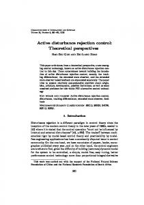
2. Benchmark Simulation Model Number 1 and Its Control Strategy 2.1. The BSM1 Introduction. BSM1 layout can be divided into two parts, which includes 5 activated sludge reactors and a secondary settler. General structure of BSM1 is shown in Figure 1. Five activated sludge reactors are called bioreactors which are composed of 2 anoxic tanks (Units 1 and 2) and 3 aerobic tanks (Units 3–5). The activated sludge model number 1 (ASM1) has been selected to describe the biological phenomena taking place in biological reactors [29, 30]. Thus, the model includes oxidizing reactions, nitrification, and denitrification for removing biological nitrogen. Behind the reactors, there is a secondary settler, which is composed of 10 layers. The 6th layer is the feed layer, through which the wastewater is from the bioreactors to the secondary settler. At last the treated wastewater comes out of the 10th layer and parts of the sludge from the 1st layer go back to Unit 1 through the external recycle. In the secondary settler, there is no biochemical reaction, just physical deposition. The doubleexponential settling velocity function has been selected to describe the secondary settler [31, 32]. In ASM1, there are 13 state variables (including 6 particulate components and 7 soluble components), 8 basic processes, 5 stoichiometric parameters, and 14 kinetic parameters. All the variables, processes, and parameters describe the oxidizing reactions, nitration reactions, and denitrification reactions. Reactions in each bioreactor about 13 state variables follow mass balancing: 𝑑𝑍𝑘 1 = (𝑄 𝑍 − 𝑟 𝑉 − 𝑄𝑘 𝑍𝑘 ) , 𝑑𝑡 𝑉𝑘 𝑘−1 𝑘−1 𝑖 𝑘
(1)
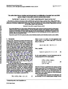
where 𝑘 is the bioreactor number, 𝑍𝑘 is the state variables, 𝑄𝑘 is the influent, 𝑉𝑘 is the volume of the bioreactor, 𝑟𝑖 is the observed conversion rates, and 𝑖 is from 1 to 13. 𝑟𝑖 is the core parameter in ASM1, which reflects the relationship among variables. BSM1 is built with Matlab/Simulink, including 5 bioreactors, a secondary settler, and a time-delay unit. The simulation data of dry weather, rainy weather, and stormy weather on benchmark of WWTPs on 14 days is provided to test the model. Only the dry weather data present in Figure 2 is used in this paper, because the data of dry weather, rainy weather, and stormy weather is the same except the last 2 two days. The flow-weighted average values of the effluent concentrations, such as chemical oxygen demand (COD), biochemical oxygen demand (BOD), ammonium (𝑆NH ), total nitrogen (TN), and total suspended solids (TSS) [1, 2], should be within the limits given in Table 1. The quality of processed
Mathematical Problems in Engineering
3 To river Qe , Ze
Secondary settler Wastewater Q0 , Z0
Biological reactor Unit 1 Unit 2
m = 10
Unit 3 Unit 4 Unit 5 Qf , Zf
Anoxic section
m=6
Aerated section Internal recycle Qa , Za
Qu , Zu
m=1 Wastage QW , ZW
External recycle Qr , Zr
Figure 1: General overview of the BSM1 plant.
3 2.5 2 1.5 1
0
2
4
6 8 10 Times (days)
12
14
140 120 100 80 60 40 20 0
300 Concentration (g/m3 )
Concentration (g/m3 )
Flow rate (m3 /d)
×104 3.5
0
2
4
6 8 10 Times (days)
SS SNH
Qa
12
SND
14
250 200 150 100 50 0
0
2
4
6
8
10
12
14
Times (days) XBH XS
Xi XS
Figure 2: Dry weather influent.
Table 1: Effluent quality limits. The variable limits Chemical oxygen demand (COD) Biochemical oxygen demand (BOD) Ammonium (𝑆NH ) Total nitrogen (TN). Total suspended solids (TSS)
Value 18 gN/m3 100 gCOD/m3 4 gN/m3 30 gSS/m3 100 gBOD/m3
wastewater called effluent quality (EQ) from the 10th layer can be described by [31] EQ =
14 days 1 [2TSS (𝑡) + COD (𝑡) + 30TN (𝑡) ∫ 7000 7 days
−20𝑆NO (𝑡) + 2BOD (𝑡)] ⋅ 𝑄𝑒 (𝑡) 𝑑𝑡, (2) where 𝑆NO is the nitrate and nitrite nitrogen. Accordingly, the influent quality (IQ) can be calculated as IQ =
14 days 1 [2TSS (𝑡) + COD (𝑡) + 30TN (𝑡) ∫ 7000 7 days
− 20𝑆NO (𝑡) + 2BOD (𝑡)] ⋅ 𝑄0 (𝑡) 𝑑𝑡. (3)
2.2. Control Strategy. In BSM1, the control of nitration reactions and denitrification reactions is important. Two factors affect the reactions. The first is the concentration of dissolved oxygen for the activated sludge process, because adequate oxygen level is good for the growth of autotrophic bacteria to reduce ammonia nitrogen to be nitrate. The other factor is the level of nitrite and nitrate in anoxic tanks. Primary control objectives have been given in Table 2 and Figure 3 shows the control structure of BSM1. Based on ASM1, the dissolved oxygen concentration in aerated sections is the key factor, which affects the process of the biochemical reactions. The dissolved oxygen concentration is manipulated by the oxygen transfer coefficient, which determines the reaction rate of the whole 13 state variables. Excessive dissolved oxygen concentration leads to increase of COD and BOD of the wastewater. On the contrary, if the dissolved oxygen concentration is relatively low, the nitration reaction is inhibited and the removal of ammonia nitrogen in the wastewater will be incomplete. The TN and 𝑆NH cannot meet the effluent requirement. Moreover, in aerated sections, keeping the proper dissolved oxygen concentration in Unit 5 is of great importance. First, the effluent quality on 7 soluble components depends on the wastewater from Unit 5, and they will not be changed in secondary settler. Second, parts of the excessive dissolved oxygen from Unit 5 to anoxic sections through the internal recycle constrain the denitrification reactions, so the control of feedback influent (𝑄𝑎 ) will keep the dissolved oxygen in a proper value in the internal recycle.
4
Mathematical Problems in Engineering Table 2: Control variables and their limitations.
Control handle Fixed oxygen transfer coefficient (𝐾𝐿 𝑎5 ) Feedback influent (𝑄𝑎 )
Limits 0∼360 0∼92230
Controlled variables Dissolved oxygen (𝑆O ) Nitrite and nitrate (𝑆NO )
Set point 2 g(-COD)/m3 1 g/m3
SO,5
Biological reactor Wastewater Q0 , Z0
Unit 1
Unit 2
Unit 3
Unit 4
Secondary settler
To river
m = 10
Qe , Ze
Unit 5
m=6 Anoxic section
Aerated section
Qf , Zf Qu , Zu
m=1 Wastage
SNO2
QW , ZW Qa , Za
Internal recycle
External recycle
Qr , Zr
Figure 3: Control strategies of BSM1.
In addition, controlling the oxygen transfer coefficient in Units 3–5 is less efficient to control the oxygen transfer coefficient in Unit 5 and make the oxygen transfer coefficient in Units 3 and 4 fixed. Therefore, the proper dissolved oxygen concentration in Unit 5 is the key factor in the whole BSM1 system. Equation (1) covers 13 state variables that meet mass balancing. However, considering the influence of the oxygen transfer coefficient (𝐾𝐿 𝑎5 ), the equation of the oxygen (𝑆O,5 ) in Unit 5 is 𝑑𝑆O,5 𝑄4 𝑆O,4 𝑄5 𝑆O,5 − + 𝑢 (𝑡) + 𝑟8 , = 𝑑𝑡 𝑉5 𝑉5
2.3. Designing the LADRC. In BSM1, (4) can be written as a first order plant (5)
where 𝑥1 = 𝑆O,5 ,
𝑄5 𝑆O,5 𝑓0 (𝑥1 ) = − , 𝑉5
𝑄4 𝑆O,4 𝑓 (𝑡) = + 𝑟8 . 𝑉5 (6)
Let 𝑄 𝑚 = − 5, 𝑉5
𝑓0 (𝑥1 ) = 𝑚𝑆O,5 = 𝑚𝑥1 .
(7)
Here, 𝑓(𝑡) is referred to as the external unknown disturbance and the internal uncertain dynamics. 𝑏0 is the compensating
𝑥2̇ = 𝜒 (𝑡) ,
𝑥1̇ = 𝑓0 (𝑥1 ) + 𝑏0 𝑢 (𝑡) + 𝑓 (𝑡) ,
𝑦 = 𝑥1 , (8)
where 𝜒 (𝑡) =
𝑑𝑓 (𝑡) . 𝑑𝑡
(9)
The state space model (8) can be written as a compact form
(4)
where 𝑉5 is the volume of Unit 5, 𝑄4 is the fluent of Unit 4, 𝑄5 is fluent of Unit 5, 𝑟8 is the observed conversion rates of the oxygen, and 𝑢(𝑡) is the oxygen transfer coefficient.
𝑥1̇ = 𝑓0 (𝑥1 ) + 𝑏0 𝑢 (𝑡) + 𝑓 (𝑡) ,
factor of the plant. Let 𝑥2 = 𝑓(𝑡), and then (5) can be written as
𝑥̇ = 𝐴𝑥 + 𝐵𝑢 (𝑡) + 𝐸ℎ,
𝑦 = 𝐶𝑥,
(10)
where 𝐴=[
𝑚 1 ], 0 0
0 𝐸 = [ ], 1
𝑏 𝐵 = [ 0] , 0
(11)
𝐶 = [1 0] .
The linear extended state observer (LESO) is designed as ̂ , 𝑧̇ = 𝐴𝑧 + 𝐵𝑢 (𝑡) + 𝐿 (𝑦 − 𝑦)
𝑦̂ = 𝐶𝑧,
(12)
where 𝑦̂ is the estimate of 𝑦. 𝐿 can be obtained using the pole placement technique, and let 𝛽 𝐿 = [ 1] . 𝛽2
(13)
The two observer poles should be placed at 𝜔𝑜 : 2
|𝜆𝐼 − (𝐴 − 𝐿𝐶)| = (𝜆 + 𝜔𝑜 ) .
(14)
Mathematical Problems in Engineering
5
LADRC r
+
−
+ −
𝜔c
1/b0
KL a5 u
BSM1
SO,5
y
(4) If 𝜔𝑜 is decreased, 𝜔𝑐 must be increased to keep the performance (see Table 3).
LESO
Figure 4: Control scheme of dissolved oxygen on BSM1.
Then, 𝛽1 and 𝛽2 can be placed at 2𝜔𝑜 + 𝑚 and 𝜔𝑜2 . Therefore, LESO is −2𝜔 1 2𝜔 + 𝑚 𝑏 𝑧̇ = [ 2𝑜 ] 𝑧 + [ 0 ] 𝑢 (𝑡) + [ 𝑜 2 ] 𝑦. 0 −𝜔𝑜 0 𝜔𝑜
(15)
The PD controller is 𝑢 (𝑡) =
(𝑟 − 𝑧1 ) 𝑘𝑑 − 𝑧2 , 𝑏0
(3) If 𝜔𝑜 ≥ 900, the disturbance is larger than the controlled signal. Performance of the closed-loop system degrades (see Figure 5(c)).
(16)
where the gain 𝑘𝑑 can be defined as the function of closedloop natural frequency 𝜔𝑐 [24]. The control scheme of dissolved oxygen in BSM1 by LADRC is given in Figure 4.
3. Simulation Results and Discussions 3.1. LADRC Parameter Tuning. In (15) and (16), 3 parameters, 𝜔𝑜 , 𝜔𝑐 , and 𝑏0 , are tunable parameters of LADRC. Integral of absolute error (IAE), integral of squared error (ISE), and variance of error (VAR) are calculated to evaluate the control of LADRC on BSM1 [2]. The optimal LADRC tuning steps are given below.
Parts of simulation results are present in Figure 5. The performance of closed-loop system and the EQ values are shown in Table 3. Comparing groups a ∼ j, one may find that as long as the dissolved oxygen concentration in Unit 5 keeps near 2g(-COD)/m3 , the EQ values are almost the same. In Table 3, the optimal parameters are shown in group e. In fact, the performances of the groups c ∼ h look the same in Figure 5. When the parameters are chosen as group e, the variation of 𝑆O,5 and 𝐾𝐿 𝑎5 is shown in Figure 6, which gives out the comparison with virtual reference feedback tuning (VRFT) [19]. The change of wastewater quality is given in Table 4. Apparently, the wastewater quality has been improved greatly. 3.2. Analysis of LADRC Parameters to BSM1. In Section 2.3, LADRC is designed based on BSM1. LESO is the key part of LADRC, which can actively estimate two states, 𝑦 and 𝑓(𝑡). The estimation errors 𝑒1 and 𝑒2 can be defined by 𝑒1 = 𝑧1 − 𝑦 = 𝑧1 − 𝑥1 , 𝑒2 = 𝑧2 − 𝑓 (𝑡) = 𝑧2 − 𝑥2 . According to (12) and (13), LESO can be rewritten as
Step 1. In (4) and (5), 𝑏0 can be set to be 1 (if the plant is unknown, 𝑏0 could be acquired by simulation).
𝑧̇1 = 𝑚𝑧1 + 𝑧2 − 𝛽1 (𝑧1 − 𝑦) + 𝑏0 𝑢 (𝑡)
Step 2. A common rule is to choose 𝜔𝑜 = 3 ∼ 5𝜔𝑐 [24]. Based on this rule, we may get a set of 𝜔𝑐 and 𝜔𝑜 that can stabilize the systems.
𝑧̇2 = −𝛽2 𝑒1 .
(a) Fixing 𝜔𝑐 , increasing and decreasing 𝜔𝑜 , we can find several groups of stable parameters named class A. (b) Fixing 𝜔𝑜 , increasing and decreasing 𝜔𝑐 , we can find another class B. (c) Comparing A and B, we may find the relationship between 𝜔𝑜 and 𝜔𝑐 . (d) Changing both 𝜔𝑐 and 𝜔𝑜 on this relationship, we may find other groups of stable parameters. Step 3. By comparison with the value of IAE, ISE, and VAR, optimal parameters can be found easily. According to the steps described above, several groups of simulation are performed, and several results can be found. (1) Dissolved oxygen concentration in Unit 5 could keep near 2g(-COD)/m3 (see Figure 5(a)) when nearly 𝜔𝑜 + 𝜔𝑐 = 1000, 𝜔𝑐 > 40, and 𝜔𝑜 < 900. (2) If 𝜔𝑜 < 200, the concentration of the dissolved oxygen fluctuates greatly (see Figure 5(b)).
(17)
= 𝑚𝑧1 + 𝑧2 − 𝛽1 𝑒1 + 𝑏0 𝑢 (𝑡) ,
(18)
Then, the differential errors are 𝑒1̇ = 𝑒2 − (𝛽1 − 𝑚) 𝑒1 ,
𝑒2̇ = −𝜒 (𝑡) − 𝛽2 𝑒1 .
(19)
When the states go into steady, that is 𝑒1̇ and 𝑒2̇ are almost zero, we have, 𝑒2 − (𝛽1 − 𝑚) 𝑒1 = 0,
−𝜒 (𝑡) − 𝛽2 𝑒1 = 0.
(20)
The errors are obtained as 𝑒1 = −
𝜒 (𝑡) , 𝛽2
𝑒2 = (𝛽1 − 𝑚) 𝑒1
(21)
𝑒2 = 2𝜔𝑜2 𝑒1 ,
(22)
which can be rewritten as 𝑒1 = −
𝜒 (𝑡) , 𝜔𝑜2
where 𝛽1 = 2𝜔𝑜 +𝑚 and 𝛽2 = 𝜔𝑜2 . If 𝜔𝑜2 ≫ −𝜒(𝑡), 𝑒1 will tend to zero and 𝑒2 will also tend to zero. In other words, LESO could
6
Mathematical Problems in Engineering
2.25
2.25 SO (g/m−3 )
2.5
SO (g/m−3 )
2.5
2 1.75 1.5
2 1.75
0
2
4
6 8 Times (days)
c d e
10
12
1.5
14
0
f g h
2
4
6 8 Times (days)
10
12
14
h i j
(a)
(b)
2.5
SO (g/m−3 )
2.25 2 1.75 1.5
0
2
4
6 8 Times (days)
10
12
14
a b
(c)
Figure 5: Comparison of the dissolved oxygen concentration in Unit 5 for different LADRC parameters.
3
300
2.8 250
2.6
200
2.2
KL a5 (1/d)
SO,5 (g/m3 )
2.4
2 1.8
150
100
1.6 1.4
50
1.2 1
7
8
9
10
11
12
13
14
0
7
8
Times (days) VRFT LADRC
9
10 11 Times (days)
VRFT LADRC
Figure 6: Comparison of 𝑆O,5 and 𝐾𝐿 𝑎5 for VRFT and LADRC.
12
13
14
Mathematical Problems in Engineering
7
Table 3: Performance indexes of the closed-loop system. 𝑏0 1 1 1 1 1 1 1 1 1 1
a b c d e f g h i j
𝜔𝑐 50 100 200 300 400 500 600 700 800 900
𝜔𝑜 950 900 800 700 600 500 400 300 200 100
IAE 0.818 0.085 0.051 0.056 0.037 0.385 0.454 0.615 0.107 0.328
ISE 0.198 0.242 0.012 0.007 0.006 0.004 0.004 0.005 0.006 0.023
Effluent 17.39 46.58 2.61 2.58 11.73 6154.12
−0.5 −1 −1.5 𝜒(t)
Influent 51.47 360.04 30.14 183.51 198.60 52089
EQ 6155.0 6153.9 6153.7 6154.1 6154.1 6153.9 6154.1 6154.2 6153.9 6154.8
×104 0
Table 4: Comparison of influent and effluent. Standers NT COD 𝑆NH BOD TSS IQ/EQ
VAR 0.01080 0.001700 0.00089 0.00050 0.00039 0.00030 0.00028 0.00028 0.00035 0.00110
−2 −2.5
estimate the 𝑦 and 𝑓(𝑡) effectively. From Section 2.3, 𝑓(𝑡) can be described by
−3 −3.5 −4
𝑄4 𝑆O,4 1 − 𝑌𝐻 𝑄4 𝑆O,4 + 𝑟8 = − 𝜌 𝑓 (𝑡) = 𝑉5 𝑉5 𝑌𝐻 1 4.75 − 𝑌𝐴 − 𝜌3 , 𝑌𝐴
0
2
4
6 8 Times (days)
10
12
14
Figure 7: Estimate of 𝜒(𝑡).
(23)
where where 𝑌𝐻 and 𝑌𝐴 are the parameters of BSM1, 𝜌1 is the basic process of aerobic growth of heterotrophs, and 𝜌3 is the basic process of aerobic growth of autotrophs:
𝜌1 =
𝑆O,5 4𝑆S,5 𝑋 𝑆S,5 + 10 𝑆O,5 + 0.2 BH,5
𝑆O,5 0.5𝑆NH,5 𝜌3 = 𝑋 , 𝑆NH,5 + 1 𝑆O,5 + 0.4 BA,5
(24)
where 𝑆S,5 is the readily biodegradable substrate in Unit 5, 𝑋BH,5 is the active heterotrophic biomass in Unit 5, 𝑆NH,5 is the nitrogen in Unit 5, and 𝑋BA,5 is the active autotrophic biomass. Then the differential of 𝑓(𝑡) is
𝜒 (𝑡) =
𝑑𝑓 (𝑡) 𝑄4 𝑑𝑆O,4 1 − 𝑌𝐻 𝑑𝜌1 4.75 − 𝑌𝐴 𝑑𝜌3 = − − , 𝑑𝑡 𝑉5 𝑑𝑡 𝑌𝐻 𝑑𝑡 𝑌𝐴 𝑑𝑡 (25)
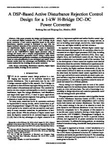
𝑆S,5 𝑑𝑋BH,5 4𝑆O,5 10𝑋BH,5 (𝑑𝑆S,5 /𝑑𝑡) 𝑑𝜌1 + = [ ], 2 𝑑𝑡 𝑆O,5 + 0.2 𝑆S,5 + 10 𝑑𝑡 (𝑆S,5 + 10) 𝑆NH,5 𝑑𝑋BA,5 0.5𝑆O,5 𝑋BA,5 (𝑑𝑆NH,5 /𝑑𝑡) 𝑑𝜌3 + = [ ]. 2 𝑑𝑡 𝑆O,5 + 0.4 𝑆 𝑑𝑡 (𝑆NH,5 + 1) NH,5 + 1 (26) 𝜌1 and 𝜌3 include the controlled state variable 𝑆O,5 . For the wastewater process being a large time-delay system, it is reasonable to let 𝑆O,5 in 𝜒(𝑡) be a small variable in [2 − Δ, 2 + Δ], where Δ leads to zero. At the same time, another variable could be estimated by a 14-day period of stabilization in closed-loop using dry weather inputs [4]. Through the simulation and calculation, 𝜒(𝑡) is described in Figure 7 with Δ about 0.2. If the parameter 𝜔𝑜 meets 𝜔𝑜2 ≫ −𝜒(𝑡), 𝜔𝑜 should exceed 160. In Section 3.1, if the parameter 𝜔𝑜 < 200, the fluctuate of the dissolved oxygen concentration becomes large. Therefore, the optimal parameters are 𝜔𝑜 = 600 and 𝜔𝑐 = 400. This 𝜔𝑜2
8 is nearly 14 times the −𝜒(𝑡). This also confirms the data given in Table 3 and the analysis above.
4. Conclusions In this paper, the control of dissolved oxygen in WWTPs is considered. The process of wastewater treatment is full of nonlinear, uncertain, and strong couplings. A robuster and more practical control strategy is in great need. As a result of the simple structure, nice disturbance rejection performance, and easy tuning approach, LADRC is employed. For the control of dissolved oxygen in WWTPs, optimal LADRC parameters tuning approach is obtained by simulations. Estimation capacity of the linear extended state observer is analyzed, which also provides a valuable guidance to choose parameters of LADRC for the control of dissolved oxygen. Simulation results confirm that LADRC is able to get a nice performance. Although the study is performed by simulation, it can be viewed as an essential step before implementing LADRC in a real plant, since BSM1 is a common framework to test control strategies for WWTPs. LADRC will probably be a more practical and promising solution to the control of wastewater treatment processes.
Conflict of Interests The authors declare that there is no conflict of interests regarding the publication of this paper.
Acknowledgments This work is supported by National Natural Science Foundation of China (51179002), Beijing Natural Science Foundation (4112017), the Importation and Development of HighCaliber Talents Project of Beijing Municipal Institutions (YETP1449).
References [1] J. B. Copp, The COST Simulation Benchmark: Description and Simulator Manual, Office for Official Publications of the European Communities, Luxembourg, Luxembourg, 2008. [2] J. Alex, L. Benedetti, J. Copp et al., Benchmark simulation model no.1 (BSM1), 2008. [3] I. R. Rodriguez-Roda, M. Sanchez-Marre, J. Comas et al., “A hybrid supervisory system to support WWTP operation: implementation and validation,” Water Science and Technology, vol. 45, no. 4-5, pp. 289–297, 2002. [4] A. Rivas, I. Irizar, and E. Ayesa, “Model-based optimization of wastewater treatment plants design,” Environmental Modelling & Software, vol. 23, no. 4, pp. 435–450, 2008. [5] G. Olsson and B. Newell, Wastewater Treatment Systems. Modelling, Diagnosis and Control, IWA Publishing, London, UK, 1st edition, 1999. [6] C. A. C. Belchior, R. A. M. Ara´ujo, and J. A. C. Landeck, “Dissolved oxygen control of the activated sludge wastewater treatment process using stable adaptive fuzzy control,” Computers & Chemical Engineering, vol. 37, pp. 152–162, 2012.
Mathematical Problems in Engineering ´ R´edey, and J. Fazakas, “Dissolved [7] B. Holenda, E. Domokos, A. oxygen control of the activated sludge wastewater treatment process using model predictive control,” Computers & Chemical Engineering, vol. 32, no. 6, pp. 1278–1286, 2008. [8] W. Shen, X. Chen, and J. P. Corriou, “Application of model predictive control to the BSM1 benchmark of wastewater treatment process,” Computers & Chemical Engineering, vol. 32, no. 12, pp. 2849–2856, 2008. [9] H.-G. Han, J.-F. Qiao, and Q.-L. Chen, “Model predictive control of dissolved oxygen concentration based on a selforganizing RBF neural network,” Control Engineering Practice, vol. 20, no. 4, pp. 465–476, 2012. [10] T. Yang, W. Qiu, Y. Ma, M. Chadli, and L. Zhang, “Fuzzy modelbased predictive control of dissolved oxygen in activated sludge processes,” Neurocomputing, vol. 136, pp. 88–95, 2014. [11] B. Carlsson and A. Rehnstr¨om, “Control of an activated sludge process with nitrogen removal—a benchmark study,” Water Science and Technology, vol. 45, no. 4-5, pp. 135–142, 2002. [12] B. Carlsson, C. F. Lindberg, S. Hasselblad, and S. Xu, “On-line estimation of the respiration rate and the oxygen transfer rate at Kungsangen wastewater plant in Uppsala,” Water Science and Technology, vol. 30, no. 4, pp. 255–263, 1994. ˚ [13] L. Amand and B. Carlsson, “Optimal aeration control in a nitrifying activated sludge process,” Water Research, vol. 46, no. 7, pp. 2101–2110, 2012. [14] M. Yong, P. Yongzhen, and U. Jeppsson, “Dynamic evaluation of integrated control strategies for enhanced nitrogen removal in activated sludge processes,” Control Engineering Practice, vol. 14, no. 11, pp. 1269–1278, 2006. [15] P. Vega, S. Revollar, M. Francisco, and J. M. Mart´ın, “Integration of set point optimization techniques into nonlinear MPC for improving the operation of WWTPs,” Computers & Chemical Engineering, vol. 68, pp. 78–95, 2014. [16] H.-G. Han, H.-H. Qian, and J.-F. Qiao, “Nonlinear multiobjective model-predictive control scheme for wastewater treatment process,” Journal of Process Control, vol. 24, no. 3, pp. 47–59, 2014. [17] J. Mendes, R. Ara´ujo, T. Matias, R. Seco, and C. Belchior, “Automatic extraction of the fuzzy control system by a hierarchical genetic algorithm,” Engineering Applications of Artificial Intelligence, vol. 29, pp. 70–78, 2014. [18] L. H. Li, X. Wang, and Y. C. Bo, “Application of adaptive dynamical programming on multivariable control of wastewater treatment process,” Computer Measurement & Control, vol. 21, no. 3, pp. 667–670, 2013. [19] J. D. Rojas, X. Flores-Alsina, U. Jeppsson, and R. Vilanova, “Application of multivariate virtual reference feedback tuning for wastewater treatment plant control,” Control Engineering Practice, vol. 20, no. 5, pp. 499–510, 2012. [20] Y.-G. Xi, D.-W. Li, and S. Lin, “Model predictive control—status and challenges,” Acta Automatica Sinica, vol. 39, no. 3, pp. 222– 236, 2013. [21] J. Q. Han, “Auto disturbances rejection controller and it’s applications,” Control and Decision, vol. 13, no. 1, pp. 19–23, 1998. [22] J. Q. Han, “Active disturbances rejection controller,” Frontier Science, vol. 1, pp. 24–31, 2007. [23] J. Q. Han, “From PID to active disturbance rejection control,” IEEE Transactions on Industrial Electronics, vol. 56, no. 3, pp. 900–906, 2009. [24] Z. Q. Gao, “Scaling and Bandwidth-Parameterization based controller tuning,” in Proceedings of the American Control Conference, Denver, Colorado, June 2003.
Mathematical Problems in Engineering [25] Y.-C. Fang, H. Shen, X.-Y. Sun, X. Zhang, and B. Xian, “Active disturbance rejection control for heading of unmanned helicopter,” Control Theory & Applications, vol. 31, no. 2, pp. 238– 243, 2014. [26] C.-E. Huang, D. Li, and Y. Xue, “Active disturbance rejection control for the ALSTOM gasifier benchmark problem,” Control Engineering Practice, vol. 21, no. 4, pp. 556–564, 2013. [27] A. Rodriguez-Angeles and J. A. Garcia-Antonio, “Active disturbance rejection control in steering by wire haptic systems,” ISA Transactions, vol. 53, no. 4, pp. 939–946, 2014. [28] L. Fucai, L. Lihuan, G. Juanjuan, and G. Wenkui, “Active disturbance rejection trajectory tracking control for space manipulator in different gravity environment,” Control Theory & Applications, vol. 31, no. 3, pp. 352–360, 2014. [29] M. Henze, W. Gujer, T. Mino et al., “Activated sludge model no.1,” IAWPRC Scientific and Technical Reports 1, 1986. [30] M. Henze, W. Gujer, T. Mino, and M. van Loosdrecht, Eds., Activated Sludge Models ASM1, ASM2, ASM2d and ASM3, IWA Publishing, IWA Task Group on Mathematical Modelling for Design and Operation of Biological Wastewater Treatment, London, UK, 2004. [31] I. Takacs, G. G. Patry, and D. Nolasco, “A dynamic model of the clarification-thickening process,” Water Research, vol. 25, no. 10, pp. 1263–1271, 1991. [32] The European cooperation in the field of scientific and technical research, Action 624: Optimal Management of Wastewater Systems, http://apps.ensic.inpl-nancy.fr/COSTWWTP/.
9
Advances in
Operations Research Hindawi Publishing Corporation http://www.hindawi.com
Volume 2014
Advances in
Decision Sciences Hindawi Publishing Corporation http://www.hindawi.com
Volume 2014
Journal of
Applied Mathematics
Algebra
Hindawi Publishing Corporation http://www.hindawi.com
Hindawi Publishing Corporation http://www.hindawi.com
Volume 2014
Journal of
Probability and Statistics Volume 2014
The Scientific World Journal Hindawi Publishing Corporation http://www.hindawi.com
Hindawi Publishing Corporation http://www.hindawi.com
Volume 2014
International Journal of
Differential Equations Hindawi Publishing Corporation http://www.hindawi.com
Volume 2014
Volume 2014
Submit your manuscripts at http://www.hindawi.com International Journal of
Advances in
Combinatorics Hindawi Publishing Corporation http://www.hindawi.com
Mathematical Physics Hindawi Publishing Corporation http://www.hindawi.com
Volume 2014
Journal of
Complex Analysis Hindawi Publishing Corporation http://www.hindawi.com
Volume 2014
International Journal of Mathematics and Mathematical Sciences
Mathematical Problems in Engineering
Journal of
Mathematics Hindawi Publishing Corporation http://www.hindawi.com
Volume 2014
Hindawi Publishing Corporation http://www.hindawi.com
Volume 2014
Volume 2014
Hindawi Publishing Corporation http://www.hindawi.com
Volume 2014
Discrete Mathematics
Journal of
Volume 2014
Hindawi Publishing Corporation http://www.hindawi.com
Discrete Dynamics in Nature and Society
Journal of
Function Spaces Hindawi Publishing Corporation http://www.hindawi.com
Abstract and Applied Analysis
Volume 2014
Hindawi Publishing Corporation http://www.hindawi.com
Volume 2014
Hindawi Publishing Corporation http://www.hindawi.com
Volume 2014
International Journal of
Journal of
Stochastic Analysis
Optimization
Hindawi Publishing Corporation http://www.hindawi.com
Hindawi Publishing Corporation http://www.hindawi.com
Volume 2014
Volume 2014