LINEAR ARRAYS WITH POLYNOMIAL PHASE DISTRIBUTION Marko Horvat, Hrvoje Domitrovic, Antonio Petosic University of Zagreb, Faculty of Electrical Engineering and Computing, Department of Electroacoustics, Unska 3, 10000 Zagreb, Croatia E- mail:
[email protected],
[email protected],
[email protected]
Abstract: Behaviour of linear arrays consisting of N+1 constantly spaced, omnidirectional radiating elements with uniform amplitude distribution and polynomial phase distribution shall be examined for the purpose of future applications to loudspeaker sound columns with the possibility of both beam steering and coverage angle control. Key words: linear arrays, phase distribution, loudspeaker sound columns
1. INTRODUCTION In most cases, the radiation pattern of a single radiating element does not meet the requirements for a certain application. Furthermore, it cannot be cha nged without serious modifications of the radiating element itself and even then the changes obtained in this manner are hardly ever satisfying. In order to obtain the desired radiation pattern, single radiating elements are assembled in one-dimensional, two-dimensional or, sometimes, threedimensional arrays. In this article calculations will be presented for one-dimensional, line array consisting of N+1 omnidirectional radiating elements with constant spacing d between the elements, as shown in Fig. 1. The amplitudes of excitation signals supplying the elements are Ai and the phases of excitation signals are ai, where i = 0, 1,..., N-1, N. Angle θ is defined as the angle between the positive z axis and the observed direction of the radiation.
Fig. 1. Linear array with constant spacing
In these calculations far- field approach shall be used, meaning that the observation point is located in the far field of the array, so all the paths between the radiating elements and the observation point are considered to be parallel. Furthermore, all path lengths are nearly the same, so there are no significant differences in signal weakening during propagation due to the differences in path lengths. The 0-th element of the array located at the point of origin is set as the reference element and the phase of the excitation signal supplying it is set to a0 = 0. In Fig.1 it can be seen that the i-th element of the array is spatially shifted with respect to the reference element for id cos θ and its excitation is phase shifted for ai, which gives the total phase shift for the i-th element di as d df δ i = i ⋅ 2π cosθ + α i = i ⋅ 2π cos θ + α i (1) λ c where λ is the wavelength, f is the frequency and c is the propagation velocity. The array factor F can be calculated as N
F = ∑ Ai e
jδi
(2)
i =0
Since the possible application of these results will be to loudspeaker sound columns, a uniform distribution of amplitudes is desired and will be discussed here. Therefore, all the excitation amplitudes Ai are set to Ai = 1, while the generality is maintained. Furthermore, the radiating elements are omnidirectional sources, so their radiation patterns have no influence on the final radiation pattern of the array; in other words, the final radiation pattern of the array is equal to the array factor F. Finally, only the absolute value of the array factor is of interest here, while the phase value is relevant only when several arrays are joined together. With these simplifications introduced, the absolute value of the array factor F | | can be calculated as: F =
N
∑e
jδi
(3)
i =0
From Eq. 1 it can be seen that there are two components responsible for the phase shift of a certain element in the array. The first one is the spatial component, dependent on the spacing of elements and the frequency on which the array operates. Unfortunately, there is not much that can be done with this component once the array is assembled. The second component is the electrical component, dependent on the phase distribution of excitation signals. This leaves lots of room for manipulating the radiation pattern of the array.
2. THEORY In most discussions about basic theory of linear arrays, only the linear phase distribution is taken into account, meaning that the electrical phase shift of the i-th element of the array is equal to ai = ki, where i = 0, 1,…, N-1, N and k is the coefficient measured in radians or degrees. This approach allows only elementary beam steering. Here a few steps further are taken by adding non- linear components into the phase distribution function. The phase distribution function is assumed to be the sum of polynomials of the following basic form:
Pj (i ) = k ji j
(4)
where k j is the coefficient of a given polynomial measured in radians or degrees, j is the degree of the polynomial ranging from 1 to n, where n is the predetermined highest degree of interest, and i is the argument which refers to the position of a given element in the array, ranging from 0 to N. All the polynomial functions defined in this manner are symmetrical with respect to the point of symmetry i S = 0, at which they take the value Pj(i S=0) = 0, i.e. the point of symmetry is the point of origin of the coordinate system, as shown in Fig. 2.
Fig. 2. Basic form polynomials Since the polynomial functions are desired to be symmetrical to the centre of the array and argument i ranges from 0 to N, it is required to shift the point of symmetry to i S = N/2. Furthermore, all polynomials are required to take the value 0 at i = 0 in order to fulfil the requirement that the electrical phase shift for the reference element remains a0 = 0, as demanded in the introduction. To meet these conditions, the polynomial functions were modified to shifted polynomial functions of the following form: j N j N PjSH (i ) = k j i − − (− 1) j 2 2
(5)
Shifted polynomial functions are shown in Fig. 3. At the point of symmetry i S = N/2, shifted polynomials take the value SH j
P
N j N = −(−1) k j 2 2
j
(6)
the sign being dependent on the sign of the coefficient k j and the degree of the polynomial. Due to the odd symmetry of odd degree shifted polynomials and the even symmetry of even degree shifted polynomials, their values for the final element of the array are SH SH N P2 j−1 (N ) = 2 ⋅ P2 j−1 2
as intended.
,
P2SHj ( N ) = 0
(7), (8)
Fig. 3. Shifted polynomials Although the coefficients k j can be chosen independently of each other, thus determining the influence of a given polynomial in the phase distribution function, in Fig. 3 the special case is shown where all shifted polynomials take the same value at the point of symmetry i S = N/2. That way the influences of all the shifted polynomials to the phase distribution function are maintained in the same order of magnitude. In order to achieve this, the value of a certain coefficient k j is given, and the values of other coefficients k m can be calculated from the following relation: m− j 2 k m = k j − , 1 < m < n, m ≠ j (9) N Finally, the phase distribution function a(i) is the sum of shifted polynomials: n
α (i ) = ∑ P j =1
j N j j N (i) = ∑ k j i − − (− 1) 2 2 j =1 n
SH j
(10)
For a given element of the array, the value of the phase distribution function becomes a(i) = ai and is entered into Eq. 1 for calculation of phase shift of a certain element of the array and, ultimately, for calculation of the array factor.
3. RESULTS After devising the polynomial phase distribution theory, actual simulations were made for the array consisting of N+1 = 8 elements, since the loudspeaker sound column, which will be built in the future, will most likely be comprised of 8 drivers, due to practical reasons. The spacing of elements was set to a real value of d = 0.085 m and the test frequency was chosen to be f = 2 000 Hz, at which the ratio d λ is equal to 0.5. Since it was desired to examine separately the influence of each polynomial, up to the sixth degree, on the radiation pattern, a group of single-polynomial phase distribution functions shown in Fig. 4 was created. The resulting radiation patterns for each phase distribution function are shown in Figs. 6 to 11. In Fig. 5 the reference radiation pattern is shown, where all the coefficients k j have the value of zero.
Fig. 4. Single-polynomial phase distribution functions
Fig. 5. Radiation pattern, k j = 0
Fig. 6. Radiation pattern, k 1 = 90°
Fig. 7. Radiation pattern, k 2 = -13°
Fig. 8. Radiation pattern, k 3 = 4°
Fig. 9. Radiation pattern, k 4 = -1°
Fig. 10. Radiation pattern, k 5 = 0.3°
Fig. 11. Radiation pattern, k 6 = -0.28°
As shown in Figs. 6, 8 and 10, the use of odd degree polynomials in the phase distribution function is required to achieve beam steering. Unfortunately, none of the odd degree polynomials, except for the first degree, i.e. the linear one, is capable of providing the desired beam steering without significant emphasizing of side lobes, which is not desirable. Even degree polynomials in the phase distribution function are directly responsible for widening the main lobe, i.e. increasing the coverage angle, as shown in Figs 7, 9 and 11. The use of any of these polynomials widens the main lobe significantly, but the absolute value of the array factor in the direction perpendicular to the array is reduced to almost half of its original value, so corrections of excitation amplitudes are required. Again, the lowest even degree polynomial has proven to be the best one, providing the widest main lobe possible while maintaining the side lobes in reasonable limits. Furthermore, if the coefficient k 2 is chosen carefully, the first side lobes can be incorporated into the main lobe, as shown in Fig. 7. In Fig. 12 several multi-polynomial phase distribution functions are shown, and the corresponding radiation patterns are shown in Figs. 13, 14 and 15.
Fig. 12. Multi-polynomial phase distribution functions
Fig. 13. Radiation pattern, k 1 = 90°, k2 = -13°
Fig. 14. Radiation pattern, k 2 = -13°, k 3 = 3°
Fig. 15. Radiation pattern, k 4 = -1°, k 5 = 0,3°, k6 = -0.1°
4. CONCLUSION In many cases, the simplest solution is proved to be the best one. As shown in the results of the simulations, linear phase distribution is the most desirable for beam steering, while higher odd degree phase distributions are not suitable for the task. As for coverage angle control, second degree, parabolic phase distribution will provide best results. Naturally, the combination of first and second degree polynomial in the phase distribution function will ensure control over both beam steering and coverage angle simultaneously, as shown in Fig. 13. While beam steering is required at all frequencies of interest, coverage angle control shall become more important as the frequency, i.e. the ratio d λ rises and the main lobe inherently becomes narrower. The goal of this study was to find a possible solution for managing the radiation pattern of a linear array, but the real benefit is the possibility of simulating any phase distribution function which can be approximated with a sum of polynomials. The study itself was conducted on a single frequency, so the next step will be to determine the polynomial coefficients as functions of frequency k j(f) in order to provide constant direction of main radiation over the whole frequency range of interest, while maintaining constant or close-to-constant coverage angle.
REFERENCES [1] E. Zentner, Antene i radiosustavi, Graphis, Zagreb, 2001. [2] M.O.J. Hawksford, Smart Digital Loudspeaker Arrays, Journal of the Audio Engineering Society, 51(12), December 2003, 1133-1162 [3] D.B. Keele, Jr., Full-Sphere Sound Field of Constant-Beamwidth Transducer (CBT) Loudspeaker Line Arrays, Journal of the Audio Engineering Society, 51(7/8), July/August 2003, 611-624