Linear discrete diffraction and transverse localization of light in two-dimensional backbone lattices Yiling Qi and Guoquan Zhang* The MOE Key Laboratory of Weak Light Nonlinear Photonics, Nankai University, Tianjin 300457, China Applied Physics School, TEDA College, Nankai University, Tianjin 300457, China School of Physics, Nankai University, Tianjin 300071, China *
[email protected]
Abstract: We study the linear discrete diffraction characteristics of light in two-dimensional backbone lattices. It is found that, as the refractive index modulation depth of the backbone lattice increases, high-order band gaps become open and broad in sequence, and the allowed band curves of the Floquet-Bloch modes become flat gradually. As a result, the diffraction pattern at the exit face converges gradually for both the on-site and off-site excitation cases. Particularly, when the refractive index modulation depth of the backbone lattice is high enough, for example, on the order of 0.01 for a square lattice, the light wave propagating in the backbone lattice will be localized in transverse dimension for both the on-site and off-site excitation cases. This is because only the first several allowed bands with nearly flat band curves are excited in the lattice, and the transverse expansion velocities of the Floquet-Bloch modes in these flat allowed bands approach to zero. Such a linear transverse localization of light may have potential applications in navigating light propagation dynamics and optical signal processing. ©2010 Optical Society of America OCIS codes: (350.5500) Propagation; (050.1970) Diffractive optics.
References and links 1. 2. 3. 4. 5. 6. 7. 8. 9. 10. 11. 12. 13. 14.
D. N. Christodoulides, F. Lederer, and Y. Silberberg, “Discretizing light behaviour in linear and nonlinear waveguide lattices,” Nature 424(6950), 817–823 (2003). J. Fleischer, G. Bartal, O. Cohen, T. Schwartz, O. Manela, B. Freedman, M. Segev, H. Buljan, and N. Efremidis, “Spatial photonics in nonlinear waveguide arrays,” Opt. Express 13(6), 1780–1796 (2005). A. L. Jones, “Coupling of Optical Fibers and Scattering in Fibers,” J. Opt. Soc. Am. 55(3), 261–269 (1965). S. Somekh, E. Garmire, A. Yariv, H. L. Garvin, and R. G. Hunsperger, “Channel optical waveguide directional couplers,” Appl. Phys. Lett. 22(1), 46–47 (1973). D. N. Christodoulides, and R. I. Joseph, “Discrete self-focusing in nonlinear arrays of coupled waveguides,” Opt. Lett. 13(9), 794–796 (1988). F. Lederer, G. I. Stegeman, D. N. Christodoulides, G. Assanto, M. Segev, and Y. Silberberg, “Discrete solitons in optics,” Phys. Rep. 463(1-3), 1–126 (2008). Y. S. Kivshar, and G. P. Agrawal, Optical solitons: from fibers to phototonic crystals (Academic Press, 2003). H. S. Eisenberg, Y. Silberberg, R. Morandotti, A. R. Boyd, and J. S. Aitchison, “Discrete Spatial Optical Solitons in Waveguide Arrays,” Phys. Rev. Lett. 81(16), 3383–3386 (1998). T. Pertsch, T. Zentgraf, U. Peschel, A. Bräuer, and F. Lederer, “Anomalous refraction and diffraction in discrete optical systems,” Phys. Rev. Lett. 88(9), 093901 (2002). H. S. Eisenberg, Y. Silberberg, R. Morandotti, and J. S. Aitchison, “Diffraction management,” Phys. Rev. Lett. 85(9), 1863–1866 (2000). J. W. Fleischer, T. Carmon, M. Segev, N. K. Efremidis, and D. N. Christodoulides, “Observation of discrete solitons in optically induced real time waveguide arrays,” Phys. Rev. Lett. 90(2), 023902 (2003). D. Neshev, E. Ostrovskaya, Y. Kivshar, and W. Krolikowski, “Spatial solitons in optically induced gratings,” Opt. Lett. 28(9), 710–712 (2003). F. Chen, M. Stepić, C. E. Rüter, D. Runde, D. Kip, V. Shandarov, O. Manela, and M. Segev, “Discrete diffraction and spatial gap solitons in photovoltaic LiNbO3 waveguide arrays,” Opt. Express 13(11), 4314–4324 (2005). D. Mandelik, H. S. Eisenberg, Y. Silberberg, R. Morandotti, and J. S. Aitchison, “Band-gap structure of waveguide arrays and excitation of Floquet-Bloch solitons,” Phys. Rev. Lett. 90(5), 053902 (2003).
#132117 - $15.00 USD
(C) 2010 OSA
Received 22 Jul 2010; revised 27 Aug 2010; accepted 28 Aug 2010; published 7 Sep 2010
13 September 2010 / Vol. 18, No. 19 / OPTICS EXPRESS 20170
15. M. J. Ablowitz, and Z. H. Musslimani, “Discrete diffraction managed spatial solitons,” Phys. Rev. Lett. 87(25), 254102 (2001). 16. N. K. Efremidis, J. Hudock, D. N. Christodoulides, J. W. Fleischer, O. Cohen, and M. Segev, “Two-dimensional optical lattice solitons,” Phys. Rev. Lett. 91(21), 213906 (2003). 17. J. W. Fleischer, M. Segev, N. K. Efremidis, and D. N. Christodoulides, “Observation of two-dimensional discrete solitons in optically induced nonlinear photonic lattices,” Nature 422(6928), 147–150 (2003). 18. Z. Chen, H. Martin, E. D. Eugenieva, J. Xu, and A. Bezryadina, “Anisotropic enhancement of discrete diffraction and formation of two-dimensional discrete-soliton trains,” Phys. Rev. Lett. 92(14), 143902 (2004). 19. X. S. Wang, A. Bezryadina, Z. G. Chen, K. G. Makris, D. N. Christodoulides, and G. I. Stegeman, “Observation of two-dimensional surface solitons,” Phys. Rev. Lett. 98(12), 123903 (2007). 20. D. N. Neshev, T. J. Alexander, E. A. Ostrovskaya, Y. S. Kivshar, H. Martin, I. Makasyuk, and Z. G. Chen, “Observation of discrete vortex solitons in optically induced photonic lattices,” Phys. Rev. Lett. 92(12), 123903 (2004). 21. X. Qi, G. Zhang, N. Xu, Y. Qi, B. Han, Y. Fu, C. Duan, and J. Xu, “Linear and nonlinear discrete light propagation in weakly modulated large-area two-dimensional photonic lattice slab in LiNbO3:Fe crystal,” Opt. Express 17(25), 23078–23084 (2009). 22. O. Borovkova, V. Lobanov, A. Sukhorukova, and A. Sukhorukov, “Discrete diffraction and waveguiding of optical beams in a cascade-induced lattice,” Bull. Russ. Acad. Sci. Phys. 72(5), 718–720 (2008). 23. O. Manela, M. Segev, and D. N. Christodoulides, “Nondiffracting beams in periodic media,” Opt. Lett. 30(19), 2611–2613 (2005). 24. R. J. Elliott, and A. F. Gibson, An Introduction to Solid State Physics and its Applications (The Macmillan Press, 1974). 25. N. K. Efremidis, S. Sears, D. N. Christodoulides, J. W. Fleischer, and M. Segev, “Discrete solitons in photorefractive optically induced photonic lattices,” Phys. Rev. E Stat. Nonlin. Soft Matter Phys. 66(4 Pt 2), 046602 (2002). 26. C. Lou, X. S. Wang, J. J. Xu, Z. G. Chen, and J. Yang, “Nonlinear spectrum reshaping and gap-soliton-train trapping in optically induced photonic structures,” Phys. Rev. Lett. 98(21), 213903 (2007). 27. N. K. Efremidis, J. W. Feischer, G. Bartal, O. Cohen, H. Buljan, D. N. Christodoulides, and M. Segev, “Introduction to Solitons in Photonic Lattices,” in Nonlinearities in Periodic Structures and Metamaterials, C. Denz, S. Flach, and Y. S. Kivshar, eds. (Springer, 2008), p. 295. 28. S. P. Guo, and S. Albin, “Simple plane wave implementation for photonic crystal calculations,” Opt. Express 11(2), 167–175 (2003). 29. K. Kawano, and T. Kitoh, Introduction to optical waveguide analysis:Solving Maxwell's Equations and the Schrodinger Equation (John Wiley & Sons, Inc., 2001). 30. B. Lv, Laser Optics: Beam Characterization, Propagation and Transformation, Resonator Technology and Physics (Higher Education Press, 2003). 31. K. M. Davis, K. Miura, N. Sugimoto, and K. Hirao, “Writing waveguides in glass with a femtosecond laser,” Opt. Lett. 21(21), 1729–1731 (1996). 32. P. R. Villeneuve, and M. Piché, “Photonic band gaps in two-dimensional square and hexagonal lattices,” Phys. Rev. B Condens. Matter 46(8), 4969–4972 (1992). 33. C. R. Rosberg, D. N. Neshev, A. A. Sukhorukov, W. Krolikowski, and Y. S. Kivshar, “Observation of nonlinear self-trapping in triangular photonic lattices,” Opt. Lett. 32(4), 397–399 (2007). 34. T. J. Alexander, A. S. Desyatnikov, and Y. S. Kivshar, “Multivortex solitons in triangular photonic lattices,” Opt. Lett. 32(10), 1293–1295 (2007). 35. O. Peleg, G. Bartal, B. Freedman, O. Manela, M. Segev, and D. N. Christodoulides, “Conical diffraction and gap solitons in honeycomb photonic lattices,” Phys. Rev. Lett. 98(10), 103901 (2007). 36. J. C. Knight, T. A. Birks, P. S. J. Russell, and D. M. Atkin, “All-silica single-mode optical fiber with photonic crystal cladding,” Opt. Lett. 21(19), 1547–1549 (1996).
1. Introduction The propagation dynamics of light in periodic lattices has been studied extensively for the intriguing discrete characteristics which are impossibly encountered in continuous media. In optics, arrays of coupled waveguides provide an excellent environment to investigate and observe the discrete dynamics, in which the mechanism that light is evanescently coupled from one site to adjacent sites profoundly alters the overall diffraction behavior of the system [1,2]. This so-called discrete diffraction can be tracked back to 1965 when Jones first theoretically addressed the issue in one-dimensional (1D) optical fiber arrays [3] and Somekh et al. observed experimentally the discrete diffraction in waveguide arrays fabricated in gallium arsenide (GaAs) a few yeas later [4]. However, because of no recognition for taking advantage of this particular diffraction process, the field remained dormant for many years until 1988 when the idea that light could be self-localized in nonlinear optical waveguide arrays [5] made the field revival again. The nonlinearly self-localized states, better known as discrete solitons (DS) [6,7], occur when the nonlinearity exactly balances the discrete
#132117 - $15.00 USD
(C) 2010 OSA
Received 22 Jul 2010; revised 27 Aug 2010; accepted 28 Aug 2010; published 7 Sep 2010
13 September 2010 / Vol. 18, No. 19 / OPTICS EXPRESS 20171
diffraction. Since then, significant progress on the studies in 1D topology has been made in the past years [8–15]. Moreover, DS in multi-dimensional lattices have attracted more attention recently, and it has been demonstrated that the light propagation dynamics in twodimensional (2D) waveguide arrays is significantly more complicated and versatile than its 1D counterpart [16–22]. In addition, nondiffracting beams in 2D linear photonic lattices have also been studied [23]. In Ref [16], a new type of 2D lattice - the backbone lattice - was investigated for supporting DS. The backbone lattice (shown in Fig. 1(a)), in which the index maxima are not isolated but resemble an array of ridge waveguides, is far different from the ordinary sinusoidal lattice (Fig. 1(b)). To date, a comprehensive description of the fundamental light diffraction features of the backbone lattice is still not available in the literature. In this paper, we investigate the linear diffraction properties of the backbone lattice in detail by considering the band structure q(kx,ky) of the extended Floquet–Bloch (FB) eigenmodes [24] of the lattice which consists of allowed bands and forbidden band gaps and determines the key features of the wave diffraction in the lattice. The paper is organized as follows: in section 2, the band structure of the spatially extended FB eigenmodes of the square backbone lattice is studied, in comparison with that of the traditional square sinusoidal lattice. In section 3, the discrete diffraction behavior with on-site excitation (the light is coupled into a single site with an index maximum) in the square backbone lattice with increasing index modulation depth is studied, the results are also compared with those in the sinusoidal lattice. In section 4, the discrete diffraction behaviors with off-site excitation (the light is injected into a single site with an index minimum) in both the square backbone and sinusoidal lattices are studied. In section 5, transverse localization of light in linear region in strongly modulated square backbone and sinusoidal lattices will be illustrated, and the underlying mechanism for this transversely localized light will be presented based on the band structures of the excited FB modes of the lattices and the light excitation configurations. In section 6, the band structure and beam diffraction features of hexagonal lattices are investigated in comparison with those of square ones. Finally, we summarize the work in section 7.
Fig. 1. Index potential of (a) a square backbone lattice and (b) a square sinusoidal lattice.
2. Band structure of the spatially extended FB eigenmodes of the square backbone lattice The evolution of the normalized slowly varying amplitude ψ(x,y,z) of the light in a 2D periodic lattice can be described by the following dimensionless equation i
∂ψ ∂z
1
+
2
∇ ⊥ψ + V ( x, y )ψ = 0, 2
(1)
where V(x,y) is a periodic index potential proportional to the refractive index modulation ∆n(x,y) of the lattice, and ∇ = ∂ ∂x + ∂ ∂y is the transverse Laplacian. For the square backbone lattice, the periodic index potential V(x,y) is given by 2
2
2
2
2
⊥
V ( x, y ) = −
V0 1 + I ( x, y )
#132117 - $15.00 USD
(C) 2010 OSA
I ( x, y )
1 + I ( x, y )
= −V0 1 −
,
(2)
Received 22 Jul 2010; revised 27 Aug 2010; accepted 28 Aug 2010; published 7 Sep 2010
13 September 2010 / Vol. 18, No. 19 / OPTICS EXPRESS 20172
where I(x,y) = A2cos2(πx)cos2(πy) is the normalized intensity of the lattice-forming beam, as in experiment the square backbone lattice can be optically induced by the interference of two or more pairs of the laser beams in photorefractive materials [17,25,26]. In our simulation, the lattice period a is set to be 11 µm, which is also served as the unit length of the whole simulation procedure, A2 is set to be 1.21, and V0 is the index potential depth, which is always negative for the backbone lattices and its magnitude controls the refractive index modulation depth of the lattice synchronously. Correspondingly, for the square sinusoidal lattice as shown in Fig. 1(b), the periodic index potential is expressed as V(x,y) = -(V0/2)(sin2(πx) + sin2(πy)), in which V0 is always positive. The solution of Eq. (1) can be expressed in the form of the spatially extended FloquetBloch eigenmodes ψ(x,y,z) = exp(-iqz)exp(ikxx + ikyy)Uk(x,y), in which Uk(x,y) possesses the same periodicity as the lattice, kx, ky are the transverse components of the Bloch wave vector, and q is the propagation constant. The band structure of the lattice can then be obtained by solving numerically the corresponding eigenvalue equation [27]: qu k +
1 2
∇ ⊥ u k + V ( x, y )u k = 0, 2
(3)
employing the plane-wave expansion (PWE) method [28]. Here the eigenfunction uk(x,y) = exp(ikxx + ikyy)Uk(x,y) obeys Bloch’s theorem. Figure 2 shows the eigenvalue bands of the propagation modes as a function of the potential depth V0 of the square backbone lattice. The bands are depicted in the multicolor regions, and the blank regions represent the band gaps. The first gap is open when the potential depth V0 is deeper than −28.4 , as already revealed in Ref [16]. Here the inset in Fig. 2 shows a magnified section of the band structure, in which the opening of the second band gap at V0 = -170.0 is illustrated. The refractive index modulation depth ∆n0 of the lattice is proportional to its index potential depth V0. For the specific experiment in Ref [17], in which the lattice was generated in a highly anisotropic SBN:75 crystal due to the photorefractive screening nonlinearity by using the optical induction technique, the refractive index modulation depth ∆n0 required to open the first and second band gaps equals to 1.05 × 10⁻⁴ [16] and 6.28 × 10⁻⁴, respectively, with an operating wavelength λ = 0.5 µm and a background refractive index n0 = 2.3, which can be acquired with typical photorefractive materials in experiment. Higher order band gaps get open in sequence with a further increase in the magnitude of the potential depth V0.
Fig. 2. The eigenvalue bands of the propagation modes as a function of the index potential depth V0 for the square backbone lattice with A2 = 1.21 and a = 11 µm. The inset is a magnified plot of the region where the second gap gets open.
Furthermore, we calculated the band structures of the square backbone lattices with various potential depth V0 along the direction Γ → X → M → Γ in the irreducible Brillouin zone (BZ), as shown in Fig. 3. The potential depth V0 of the backbone lattice is set to be −5 , −50 and −200 for Figs. 3(a)-3(c), corresponding to the refractive index modulation depth ∆n0
#132117 - $15.00 USD
(C) 2010 OSA
Received 22 Jul 2010; revised 27 Aug 2010; accepted 28 Aug 2010; published 7 Sep 2010
13 September 2010 / Vol. 18, No. 19 / OPTICS EXPRESS 20173
of 2.24 × 10⁻⁵, 2.24 × 10⁻⁴ and 8.95 × 10⁻⁴ with the aforementioned parameters of SBN:75 crystal, respectively. The potential depths are selected in such a way that no band gap is open for the V0 = −5 case (see Fig. 3(a)); the first band gap gets open while the second band gap is still not for the V0 = −50 case (see Fig. 3(b)); and for the V0 = −200 case both the first and the second band gaps are already open, as shown in Fig. 3(c). In comparison, we also give the band structure of the square sinusoidal lattice with a potential depth V0 = 90.4 in Fig. 3(d). For a Kerr-type optical lattice where V0 = (2πn0a/λ)2∆n0 [16,17], the corresponding refractive index modulation depth would be 8.95 × 10⁻⁴ with λ = 0.5 µm and n0 = 2.3. As is seen, with the same refractive index modulation depth, the gaps in the sinusoidal lattice are much broader than those in the backbone one. We also notice that the allowed band curves become flatter with the increase of the magnitude of the potential depth, which will have a significant effect on the light propagation dynamics in the periodic lattices, as we will discuss in detail in the following sections.
Fig. 3. The band structures of the spatially extended FB modes along the direction Γ → X → M → Γ in the irreducible BZ of the square backbone lattices with the index potential (a) V0 = −5, (b) V0 = −50, and (c) V0 = −200, respectively. For comparison, the band structure of a square sinusoidal lattice with an index potential V0 = 90.4 is also shown in (d).
3. Beam diffraction features in the square backbone lattice with on-site excitation The light wave propagation dynamics in the square backbone lattice is then studied numerically by use of the beam propagation method (BPM) [29,30]. In the simulation, a Gaussian beam with a waist equal to one lattice period is coupled into the lattice, the wavelength of the beam is set to be λ = 0.5 µm. The beam propagates in the lattice for 6000 unit length, corresponding to a total propagation length of 6.6 cm in real space. Figure 4 shows the linear diffraction features of light in square backbone lattices with various index potential depth V0 for the on-site excitation case, in which the index potential depth V0 is −5 for Figs. 4(a)-4(b), −50 for Figs. 4(c)-4(d), and −200 for Figs. 4(e)-4(f), respectively. The corresponding band structures of the backbone lattices are shown in Figs. 3(a)-3(c). Here Figs. 4(a), 4(c) and 4(e) reveal the intensity distribution patterns at the exit face of the backbone lattices, and Figs. 4(b), 4(d) and 4(f) indicate the beam propagation dynamics in the y = −1/2 slice (since for on-site excitation in the square backbone lattice, the beam is focused into the index maximum at position (−1/2,-1/2) according to the coordinates in Fig. 1(a)). For comparison, the intensity distribution pattern at the exit face and the beam propagation
#132117 - $15.00 USD
(C) 2010 OSA
Received 22 Jul 2010; revised 27 Aug 2010; accepted 28 Aug 2010; published 7 Sep 2010
13 September 2010 / Vol. 18, No. 19 / OPTICS EXPRESS 20174
dynamics in the y = 0 plane in the square sinusoidal lattice with a potential depth V0 = 90.4 for the on-site excitation case are also depicted in Figs. 4(g)-4(h). For the sinusoidal lattice the incident beam is focused into the index maximum at position (0,0) according to the coordinates in Fig. 1(b), so that the light propagation slice is chosen as the y = 0 plane. It is seen that, for both the square backbone and sinusoidal lattices, the beam propagation dynamics shows typical discrete diffraction characteristics in all cases with on-site excitation, which is very different from the diffraction behavior in the homogeneous media. More interestingly, although the ridge waveguide arrays in the backbone lattices are connected with each other, it is revealed clearly that the beam in the backbone lattice becomes more and more converged as the refractive index modulation depth increases. We believe that this convergence behavior is mainly due to the confinement effect originating from the flat tendency of the excited band curves. As shown in Fig. 3, with the increase of the refractive index modulation depth, high-order gaps get open in sequence and the allowed bands become flat gradually. Since the transverse expansion velocity of the light propagating in the lattice is proportional to the differential ∂q/∂k⊥, in which k = k + k ⊥
2
2
x
y
is the magnitude of the
transverse Bloch wave vector, the transverse expansion of the FB modes will be significantly suppressed with flat band profiles. In particular, the light can be localized transversely in the lattice even in linear region when the refractive index modulation depth is high enough, which will be discussed in detail in section 5. Note that such a convergence effect is more effective in the sinusoidal lattice due to broader band gaps and flatter allowed bands (see Fig. 3(d)), as compared to that of the backbone lattice (see Fig. 3(c)) with the same refractive index modulation depth. 4. Beam diffraction features in the square backbone lattice with off-site excitation We then investigate the cases with off-site excitation, namely, when the light is focused into the low index site of the lattice. Except for the location of the incidence, all other parameters remain the same as those in the previous simulations in section 3. Figures 5(a)-5(f) show the diffraction features of light in the square backbone lattices in the off-site excitation case with the same potential depths as those in Figs. 3 and 4, in which the intensity distribution patterns at the exit face are shown in Figs. 5(a), 5(c) and 5(e), and the beam propagation dynamics in the y = 0 slice is shown in Figs. 5(b), 5(d) and 5(f) (For off-site excitation, the light is focused into the site with an index minimum at position (0,0) according to the coordinates in Fig. 1(a)). For comparison, we also study the light propagation dynamics in the off-site excitation case in the square sinusoidal lattice with V0 = 90.4. The intensity distribution of the diffraction pattern at the exit face and the beam propagation dynamics in the y = −1/2 slice are respectively shown in Fig. 5(g) and Fig. 5(h), which hold the similar diffraction patterns as those with on-site excitation in the sinusoidal lattice (see Figs. 4(g)-4(h)). One sees that the diffraction pattern and the propagation dynamics of light with off-site excitation also possess typical characteristics of discrete diffraction in periodic lattices. The light propagating in the square backbone lattices in the off-site excitation case spreads not only in the diagonal direction but also in the orthogonal direction, which becomes remarkable especially when the magnitude of the index potential depth gets larger. The peculiarity of the diffraction feature in the backbone lattice here is that, even if the low index sites of the backbone lattice are isolated with each other, the light launched into a single low index site spreads first into the nearest neighboring high index sites as it propagates. The final output intensity distribution at the exit face of the backbone lattice in the off-site excitation case is the result of coherent superposition of four nearest on-site excitations around the initial low index site, as clearly shown in Fig. 7(a) in the next section. As is the case for the on-site excitation, the light also converges gradually in the transverse dimension with off-site excitation in both the square backbone and sinusoidal lattices as the refractive index modulation depths of the lattices increase.
#132117 - $15.00 USD
(C) 2010 OSA
Received 22 Jul 2010; revised 27 Aug 2010; accepted 28 Aug 2010; published 7 Sep 2010
13 September 2010 / Vol. 18, No. 19 / OPTICS EXPRESS 20175
Fig. 4. Discrete diffraction behaviors in the square backbone and sinusoidal lattices with on-site excitation. Light propagates in the lattices with 6000 unit length. The index potential depth V0 of the backbone lattice is −5 for (a) and (b), −50 for (c) and (d), −200 for (e) and (f), respectively. For comparison, discrete diffraction behavior of light in the sinusoidal lattice with V0 = 90.4 in the on-site excitation case is shown in (g) and (h). Here (a), (c), (e) and (g) depict the intensity distribution patterns at the exit face of the lattices. (b), (d) and (f) show the beam propagation dynamics in the y = −1/2 slice of the backbone lattices, while (h) describes the beam propagation dynamics in the y = 0 plane of the sinusoidal lattice.
#132117 - $15.00 USD
(C) 2010 OSA
Received 22 Jul 2010; revised 27 Aug 2010; accepted 28 Aug 2010; published 7 Sep 2010
13 September 2010 / Vol. 18, No. 19 / OPTICS EXPRESS 20176
Fig. 5. Discrete diffraction behaviors in the square backbone and sinusoidal lattices with offsite excitation. Light propagates in the lattices with 6000 unit length. The index potential depth V0 of the backbone lattice is −5 for (a) and (b), −50 for (c) and (d), and −200 for (e) and (f), respectively. For comparison, discrete diffraction behavior of light in the sinusoidal lattice with V0 = 90.4 in the off-site excitation case is shown in (g) and (h). Here (a), (c), (e) and (g) are intensity distribution patterns at the exit face of the lattices; while (b), (d) and (f) show the beam propagation dynamics in the y = 0 slice and (h) is the light propagation dynamics in the y = −1/2 slice of the lattice.
5. Transverse localization of light in highly modulated square lattices As described in sections 3 and 4, the light converges gradually in the transverse dimension in both the square backbone and sinusoidal lattices as the refractive index modulation depths of the lattices increase. In this section, we further study the light propagation dynamics in highly modulated square lattices. Surprisingly, we find that the light can be localized transversely in two dimension even in the square backbone lattices, no matter with on-site or off-site excitation, when the refractive index modulation depth is high enough, i.e., up to a value on
#132117 - $15.00 USD
(C) 2010 OSA
Received 22 Jul 2010; revised 27 Aug 2010; accepted 28 Aug 2010; published 7 Sep 2010
13 September 2010 / Vol. 18, No. 19 / OPTICS EXPRESS 20177
the order of 0.01, though the high refractive index ridges in the square backbone lattices are connected with each other and look like arrays of planar waveguides.
Fig. 6. The band structure diagram of (a) the square backbone lattice and (d) the square sinusoidal lattice with a refractive index modulation depth ∆n0 = 0.0224, the intensity distribution at the exit face after 6000 unit propagation length in (b) the backbone lattice and (e) the sinusoidal lattice, and the light propagation dynamics (c) in the y = −1/2 slice in the backbone lattice and (f) in the y = 0 slice in the sinusoidal lattice with on-site excitation. The dashed blue curves in (a) and (d) represent the propagation constants determined by Snell’s law and reachable by the exciting beam.
Figure 6 shows the band structures of the square lattices in the irreducible BZ, the output intensity distribution and the light propagation dynamics with on-site excitation for both the backbone lattice (Figs. 6(a)-6(c)) and the sinusoidal lattice (Figs. 6(d)-6(f)), respectively, in which Figs. 6(a) and 6(d) are the band structures of the FB modes, Figs. 6(b) and 6(e) are the 2D output intensity distribution, and Fig. 6(c) is the light propagation dynamics in the y = −1/2 slice in the square backbone lattice while Fig. 6(f) is the propagation dynamics in the y = 0 slice in the square sinusoidal lattice. The propagation length is also 6000 unit length and the refractive index modulation depth is set to be ∆n0 = 0.0224, corresponding to an index potential depth V0 = −5000 for the backbone lattice and V0 = 2263.4 for the sinusoidal lattice according to the aforementioned proportional relations between the refractive index modulation depth and the index potential depth in section 2. Although a lattice with a refractive index modulation depth on the order of 0.01 may not be produced in typical photorefractive crystals by using the optical induction technique, it may be written directly through multi-photon-induced refractive index changes using a focused femtosecond laser beam [31]. The light excitation condition here is the same as that in Fig. 4. We note that in the highly modulated lattices, more band gaps get open and become much broader, meanwhile, the allowed band curves become flatter. When the light is coupled into a single high index site, it will excite only a limited set of FB modes of the lattices with the propagation constant q below the dashed blue curves which are determined by Snell’s law and can be expressed analytically as q = k − k − k + V 2
q
=
k − kx − ky 2
2
2
2
2
x
y
0
for the backbone lattice and
for the sinusoidal lattice, as indicated in Figs. 6(a) and 6(d), respectively.
Note that there is a biased constant index potential V0 for the backbone lattice, as can be seen from Eqs. (2) and (3). It is seen that the band curves of the excited FB modes are nearly flat, indicating that the transverse expansion velocities of these FB modes approach to zero and the transverse expansion of the beam in the lattice almost stops, therefore, the light coupled into
#132117 - $15.00 USD
(C) 2010 OSA
Received 22 Jul 2010; revised 27 Aug 2010; accepted 28 Aug 2010; published 7 Sep 2010
13 September 2010 / Vol. 18, No. 19 / OPTICS EXPRESS 20178
the lattices is localized in the transverse dimension. On the other hand, in an analogy to the periodic finite potential well in quantum mechanics, with the increase in the potential depth of the periodic well, spatially localized states associated with discrete energy levels will appear in the well (see Eq. (3)). More interestingly, with a further increase in the refractive index modulation depth, it is possible to selectively excite the FB modes within the lowest allowed band. The transverse localization of light in the highly modulated square lattices occurs not only in the on-site excitation case but also in the off-site excitation case. Figure 7 shows the transverse localization of light propagating in both the square backbone and sinusoidal lattices with off-site excitation. The simulation parameters of the light and the lattices are the same as those in Fig. 6 except that the light is injected into a single low index site in the off-site excitation case. It is numerically confirmed that the light is first coupled into the nearest four neighboring high index sites during its initial propagation stage in the lattices, and then it propagates along the high index sites while localized transversely.
Fig. 7. Intensity distribution at the exit face of (a) the square backbone lattice and (b) the square sinusoidal lattice with off-site excitation. Other parameters of the light and the lattices are the same as those in Fig. 6.
6. Band structure and beam diffraction features in hexagonal lattices It is well known that the hexagonal lattice supports larger band gaps [32–34], therefore, it is natural to ask whether or not the linear transverse localization of light can be realized more easily in the hexagonal lattices. Furthermore, such hexagonal lattices can be produced either by the optical induction technique [33,35] or by stacking fibers just as in the fabrication of photonic crystal fibers [36]. In this section, we will focus our attention on the band structure and the beam diffraction behaviors in both the hexagonal backbone and sinusoidal lattices. Theoretically, the index potential V(x,y) of the hexagonal backbone lattice can also be expressed by Eq. (2) but with a normalized lattice-forming beam intensity in the form of 2 1 1 I ( x, y ) = A2 cos 2 π x cos 2 − π x − π y cos 2 − π x + π y . Figure 8(a) shows the 3 3 3 structural sketch of the index potential of a hexagonal backbone lattice with A2 = 1.21 and a lattice period a = 11 µm. Meanwhile, the eigenvalue bands of the propagation modes as a function of the potential depth V0 of the hexagonal backbone lattice is also shown in Fig. 8(b), in which the inset is a magnified plot of the region where the second band gap is open. We note that the first band gap is open at V0 = −9, and the second band gap gets open at V0 = −90, respectively. It is evident that the index potential depths required to open the band gaps in the hexagonal backbone lattice are indeed much lower than those of the square backbone lattice with the same lattice period (see Fig. 2), just as the case for the hexagonal sinusoidal lattices [33,34].
#132117 - $15.00 USD
(C) 2010 OSA
Received 22 Jul 2010; revised 27 Aug 2010; accepted 28 Aug 2010; published 7 Sep 2010
13 September 2010 / Vol. 18, No. 19 / OPTICS EXPRESS 20179
Fig. 8. (a) Index potential and (b) the eigenvalue bands of the propagation modes as a function of the potential depth V0 for the hexagonal backbone lattice with A2 = 1.21 and a = 11 µm. The inset in (b) is a magnified plot of the region where the second gap gets open.
Surprisingly but interestingly, we find that the discrete diffraction in the hexagonal backbone lattice is more prominent than that in the square one. Figure 9(a) shows the intensity distribution pattern at the exit face of the hexagonal backbone lattice with the index potential depth V0 = −5000 for the on-site excitation case. The light propagates in the lattice with 6000 unit length. It is clearly seen that the light propagation is still of typical discrete diffraction characteristics in the hexagonal backbone lattice with V0 = −5000, in strong contrast to the transversely localized state of light in the square backbone lattice with the same potential depth (Fig. 6(b)). The reason is that more propagation modes are excited and the transverse expansion velocities of the excited FB modes are much larger in the hexagonal backbone lattice as compared to those in the square backbone lattice. Figures 9(b) and 9(c) show the band profile of the first band along the direction Γ → X → M → Γ in the irreducible BZ for the hexagonal and square backbone lattices, respectively, with V0 = −5000. The transverse expansion velocities of the FB modes near the M symmetric point in the hexagonal backbone lattice are found to be about 12 times larger than those in the square backbone lattice. This means that larger index potential depth is required to localize the light transversely in the hexagonal backbone lattice as compared to the square backbone lattice. As an example, Fig. 10 shows the band structure of the hexagonal backbone lattice with V0 = −60000 and the 2D output intensity distribution at a propagation length of 6000 unit length with on-site and offsite excitation, respectively. As expected, the band curves of the FB modes become much flatter in this case and the light is nearly localized in two transverse dimensions in the hexagonal backbone lattice with both on-site and off-site excitation.
Fig. 9. (a) Intensity distribution pattern at the exit face of the hexagonal backbone lattice with a potential depth V0 = −5000 and a propagation length of 6000 unit length for the on-site excitation case, and the profile of the first band of the FB modes along the direction Γ → X → M → Γ in the irreducible BZ of (b) the hexagonal backbone lattice and (c) the square backbone lattice.
#132117 - $15.00 USD
(C) 2010 OSA
Received 22 Jul 2010; revised 27 Aug 2010; accepted 28 Aug 2010; published 7 Sep 2010
13 September 2010 / Vol. 18, No. 19 / OPTICS EXPRESS 20180
Fig. 10. (a) The band structure of the FB modes in the hexagonal backbone lattice with an index potential depth V0 = −60000. The dashed blue curve represents the propagation constants determined by Snell’s law and reachable by the exciting beam. The 2D output intensity distribution with a propagation length of 6000 unit length is shown in (b) with on-site excitation and (c) with off-site excitation.
In a similar way, the hexagonal sinusoidal lattice can be constructed theoretically with an V 2 1 1 π x + sin 2 − π x − π y + sin 2 − π x + π y . index potential V ( x, y ) = − 0 sin 2 2 3 3 3 We confirm numerically that the hexagonal sinusoidal lattice does support larger band gaps [32–34]. On the other hand, in contrast to the prominent discrete diffraction in the hexagonal backbone lattice, the light can be localized transversely in the hexagonal sinusoidal lattice, even much easier than in the square sinusoidal lattice. Figure 11(a) shows the band structure of a hexagonal sinusoidal lattice with an index potential depth V0 = 2263.4 and with a lattice period a = 11 µm, where the inset shows the index potential structural sketch of the hexagonal sinusoidal lattice. Again, the blue dashed curve represents the propagation constants determined by Snell’s law and reachable by the exciting beam. We note that only the first band of the FB modes with a flat band profile can be excited in this case, indicating that the light will be transversely localized in the lattice with both on-site and off-site excitation, as shown clearly in Figs. 11(b) and 11(c), respectively.
Fig. 11. (a) The band structure of the FB modes in the hexagonal sinusoidal lattice with the potential depth V0 = 2263.4 and a lattice period a = 11 µm, in which the inset shows the index potential structural sketch of the lattice. The 2D output intensity distribution with a propagation length of 6000 unit length is shown in (b) with on-site excitation and (c) with off-site excitation.
7. Conclusions
In conclusion, we have investigated the linear discrete diffraction features of light in the backbone lattices with both on-site and off-site excitation. Our results clearly show that, with the increase of the refractive index modulation depth of the backbone lattice, high-order band gaps get open in sequence, the band gaps become larger, moreover, the allowed band curves of FB modes become flatter. This makes the transverse expansion velocity of the light coupled into a single lattice site become slower, so that the light converges as the refractive index modulation depth increases. Especially, when the refractive index modulation depth of the backbone lattice is high enough, for example, on the order of 0.01 for the square lattice and
#132117 - $15.00 USD
(C) 2010 OSA
Received 22 Jul 2010; revised 27 Aug 2010; accepted 28 Aug 2010; published 7 Sep 2010
13 September 2010 / Vol. 18, No. 19 / OPTICS EXPRESS 20181
0.1 for the hexagonal lattice, only a limited set of FB modes with nearly flat band curves are excited, and the light can be localized in the transverse dimension during its propagation in the backbone lattices no matter with on-site or off-site excitation. As compared to the case in the square backbone lattice, larger refractive index modulation depth is required to observe the transverse localization of light in the hexagonal backbone lattice. The phenomenon also occurs in the highly modulated sinusoidal lattices with both square and hexagonal geometries. This linear transverse localization of light in highly modulated periodic lattices can also be understood in an analogy to the spatially localized states associated with the discrete energy levels in a periodic potential well in quantum mechanics. Such transverse localization of light is interesting not only from a fundamental point of view, but also from a practical application point of view, because it is more stable without the involvement of optical nonlinearity and can be designed at will, and therefore may have important potential applications in manipulating the light propagation dynamics and optical signal processing. Acknowledgements
This work is supported financially by the MOE Cultivation Fund of the Key Scientific and Technical Innovation Project (708022), the NSFC (90922030, 10904077, 10804054), the 111 project (B07013), the 973 program (2007CB307002), the CNKBRSF (2006CB921703) and the Fundamental Research Funds for the Central Universities.
#132117 - $15.00 USD
(C) 2010 OSA
Received 22 Jul 2010; revised 27 Aug 2010; accepted 28 Aug 2010; published 7 Sep 2010
13 September 2010 / Vol. 18, No. 19 / OPTICS EXPRESS 20182