Linear Maps - Microsoft

Linear Maps Shuvendu K. Lahiri

Shaz Qadeer

David Walker

Microsoft Research [email protected]

Microsoft Research [email protected]

Princeton University [email protected]

Abstract Verification of large programs is impossible without proof techniques that allow local reasoning and information hiding. In this paper, we resurrect, extend and modernize an old approach to this problem first considered in the context of the programming language Euclid, developed in the 70s. The central idea is that rather than modeling the heap as a single total function from addresses (integers) to integers, we model the heap as a collection of partial functions with disjoint domains. We call each such partial function a linear map. Programmers may select objects from linear maps, update linear maps or transfer addresses and their contents from one linear map to another. Programmers may also declare new linear map variables, pass linear maps as arguments to procedures and nest one linear map within another. The program logic prevents any of these operations from duplicating locations and thereby breaking the key heap representation invariant: the domains of all linear maps remain disjoint. Linear maps facilitate modular reasoning because programs that use them are also able to use the simple, classical frame and anti-frame rules to preserve information about heap state across procedure calls. We illustrate our approach through examples, prove that our verification rules are sound, and show that operations on linear maps may be erased and replaced by equivalent operations on a single, global heap.

1. Introduction Verification of large programs is impossible without proof techniques that allow local reasoning and information hiding. In this paper, we resurrect, extend and modernize an old approach to this problem first considered in the context of the programming language Euclid [19, 22], developed in the 70s. This approach centers around the introduction of a new data type, which we call a linear map. Intuitively, linear maps are simply little heaplets: Programmers may store objects in linear maps, look up objects in linear maps and, most interestingly, transfer addresses from one linear map to another. Programmers may also declare new linear map variables, pass them as arguments to functions, receive them as results, or nest them within one another. We call these maps linear because of their connection to linear type systems [13, 30, 31]: like values with linear type, linear maps are never duplicated nor aliased. Programs that use linear maps tend to be written in a functional store-passing (i.e., linear-map-passing) style as this style facilitates local reasoning and information hiding. However, despite this functional facade, linear maps programs are actually ordinary imperative programs that load from, and store to, a single, global heap. In order to connect a linear maps program to its corresponding conventional imperative program, we define an erasure transformation that erases all linear maps variables, erases all transfer operations and replaces linear map lookups and updates with lookups and updates on the global heap. In the forward direction, the erasure transformation shows that using linear maps incurs no overhead; they

are really just a new kind of ghost variable, used, as ghost variables often are, to facilitate modular verification. In the reverse direction, the erasure transformation may be seen as a tactic for proving the correctness of ordinary imperative programs: given an ordinary program, the reverse transformation explains the legal ways to transform it into an easy-to-verify linear maps program without changing its operational behavior. There are a number of reasons we believe researchers should adopt linear maps as a modular verification technology. First and foremost, the idea is surprisingly simple to understand, to implement and, we hope, to build upon. We believe this is a key contribution. Second, linear maps require no new language of assertions. Generated verification conditions are encoded in first-order logic and may be solved by off-the-shelf SMT solvers such as Z3 [8]. Third, using linear maps enables effective use of the classical frame and anti-frame rules, completely unchanged, despite the presence of an imperative heap. Fourth, linear maps technology requires no changes to the overall judgmental apparatus involved in standard, first-order verification condition generation: it does not use nonstandard modifies clauses and it does not depend upon sophisticated auxiliary notions such as the footprint or frame of a formulae. Consequently, it should be relatively easy to extend any one of a number of standard, existing verification condition generation tools with these new data types. Our work on linear maps has been directly inspired by several other recent approaches to modular reasoning, including research on Separation Logic [15, 25, 24], Dynamic Frames [17, 20] and Region Logic [1]. The advantages of linear maps over these previous approaches are their simplicity and the minimalism of the required extensions over standard first-order Floyd-Hoare logic. For example, Separation Logic achieves its goals at the expense of introducing a new set of assertions involving the separating conjunction F1 ∗ F2 — assertions that cannot be proven directly by classical off-the-shelf first-order theorem provers. Alternatively, Dynamic Frames and Region Logic operate by changing classical concepts such as the modifies clause, tracking exotic effects, or developing new footprint analyses. Linear maps are also closely connected to research done on the Euclid programming language in the 70s. Euclid contained a data type called a “collection” and each pointer was associated, via its static type, with such a collection. Such collections are similar to the linear maps developed in this report, and one of the important contributions of our work is to resurrect this basic idea, which the research community had almost entirely forgotten. In addition, however, we have presented the theory in a modern style, added critical new operations on linear maps, developed a logic tailored for modern SMT solvers, outlined the connection to Separation Logic and its frame rules, and proven important technical results including soundness and erasure theorems. The rest of the paper is organized as follows. Section 2 presents the central concepts in greater depth. Section 3 presents the tech-

procedure incr(int p) returns () modifies heap { heap[p] := heap[p] + 1; } heap[py] := 42; call incr(px);

Figure 1. Frame rule with ordinary maps

procedure incr(p: int, t:lin) requires p ∈ dom(t) ensures p ∈ dom(t) { t[p] := t[p] + 1; } l[py] := 42; var lx:lin in lx := l@{px}; call incr(px,lx); l := lx@{px};

nical details. Section 4 explains some interesting extensions. Sections 5 and 6 discuss related work in greater depth and conclude.

Figure 2. Frame rule with linear maps

2. Key Concepts

2.1 Linear Maps

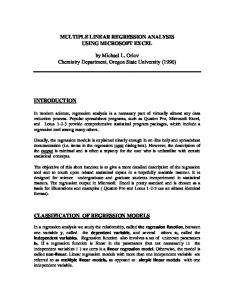
Two structural verification rules are required to verify just about any imperative program. The first is the rule of consequence, which states that if a Floyd-Hoare triple {P }C{Q} is valid and P ′ ⇒ P and Q ⇒ Q′ then the triple {P ′ }C{Q′ } is also valid. The second is the (classical) frame rule, which states that if {P }C{Q} is valid and the set of variables modified by C is disjoint from the set of free variables of R then {R ∧ P }C{R ∧ Q} is also valid. In other words, the validity of framing formula R may be preserved across any statement that does not modify the frame’s free variables. With that background, consider the procedure incr:

We address this weakness of the conventional frame rule, not by changing it, but by refining our modeling of the heap. Instead of modeling the heap with a single monolithic map, we model it as a collection of partial maps with disjoint domains. We call each such map a linear map, which is essentially a pair comprising a total map representing the contents and a set representing the domain of the linear map. We refer to the underlying total map and domain of a linear map ℓ as map(ℓ) and dom(ℓ) respectively. We augment our programming language with operations over linear maps that are guaranteed to preserve the invariant that the domains of all linear maps are pairwise disjoint and their union is the universal set. We refer to this invariant as the disjoint domains invariant. We now rewrite the program from Figure 1 using linear maps as shown in Figure 2. As we explain in Section 2.2, the program in Figure 1 can be obtained from the program in Figure 2 using the erasure operation; consequently, any properties about the runtime behavior of the latter program are valid for the former as well. The new definition of procedure incr takes a pointer p and a linear map t as arguments.1 The implementation of incr demonstrates that linear maps can be read and written just like ordinary maps. Unlike ordinary maps, a read or a write of a linear map t at the address p comes with the precondition that p is in the domain t. The read and write of t[p] performed during the increment operation are safe because of the precondition of incr. Let D denote the code fragment in Figure 2 after the definition of incr. The contents of the heap at the beginning of D is modeled by the linear map l whose domain includes both addresses px and py. In order to call incr with the pointer px, we also need to pass in a linear map whose domain contains the address px. We create such a linear map by declaring a new variable lx, whose domain is empty initially. We then perform the transfer statement lx := l@{px} to move the contents of address px from l to lx; this operation has the precondition that px is in the domain of l. The linear map lx is now passed, along with the pointer px to incr, thus satisfying the precondition of incr. It is important to note that the procedure call has a side effect on the variable lx passed for the linear argument t. At entry, the contents of lx are transferred into t; at exit, the contents of t are transferred back into lx. This operational behavior is essential to maintain the disjoint domains invariant. After the call, we transfer the pointer px from lx to l. Thus, there is an implicit modifies clause on linear map arguments for a procedure that we do not explicitly show. Unlike the previous version of the incr procedure in Figure 1, the new version of incr has the empty modifies specification.

procedure incr() returns () requires true, ensures true, modifies x { x := x + 1; }

This procedure has no input arguments and no output arguments. Its specification consists of the precondition true, the postcondition true, and the guarantee that it does not modify any variable except x. Henceforth, our examples will use the convention that a missing requires clause indicates the precondition true, a missing ensures clause indicates the postcondition true, and a missing modifies clause indicates that the procedure does not modify any variables in the caller’s scope. Consider a call to incr in a calling scope that contains another variable y. The Floyd-Hoare triple {y = 42} call incr() {y = 42} is easily proved through a combination of the conventional frame and consequence rules. {true} call incr() {true} ---------------------------------------- (Frame) {y=42 ∧ true} call incr() {y=42 ∧ true} ---------------------------------------- (Consequence) {y=42} call incr() {y=42}

The main reason for the simplicity of the proof is that the set of variables modified by the code fragment call incr() is disjoint from the free variables in the assertion y = 42. This simple proof strategy does not quite work when the heap is used to allocate data. The standard method of modeling a heap [5] uses a single map variable mapping memory addresses to their contents. Since a procedure that updates the heap at any address must contain the map variable in its modifies set, the conventional frame rule cannot be used for preserving heap-related assertions across a call to such a procedure. To illustrate the problem, we model the heap as a variable heap mapping int to int and allocate the variables x and y on the heap with distinct addresses px and py (Figure 1). Further, we change the procedure incr to take the memory address whose contents are to be incremented. Let C denote the code fragment in Figure 1 after the definition of incr. Then, the triple {px != py} C {heap[py] = 42} can not be proved using the conventional frame rule.

1 tot

and lin denote the types of ordinary and linear maps from int to int respectively.

procedure incr(p: int, tm:tot, t:lin) requires p ∈ dom(t) ∧ tm = map(t) ensures p ∈ dom(t) ∧ t[p] = tm[p]+1 { t[p] := t[p] + 1; }

{ px != py ∧ l[py] 7→

∧ l[px] 7→

}

l[py] := 42; { px != py ∧ l[py] 7→ 42 ∧ l[px] 7→

}

l[px] := 24; l[py] := 42; l[px] := 24; var lx:lin in lx := l@{px}; var lxm:tot in lxm := map(lx); call incr(px,lxm,lx); l := lx@{px};

{ px != py ∧ l[py] 7→ 42 ∧ l[px] 7→ 24 } var lx:lin in { px != py ∧ l[py] 7→ 42 ∧ l[px] 7→ 24 } lx := l@{px}; { px != py ∧ l[py] 7→ 42 ∧ lx[px] 7→ 24 }

Figure 3. Ghost variables

var lxm:tot in

Consequently, the triple {px != py} C {l[py] = 42} can be easily verified using the conventional frame rule. 2.2

lxm := map(lx);

Erasure

An important aspect of our system is the erasure operation which allows us to connect the operational semantics of the program written using linear maps with the corresponding program written using a global total map. As an example, the erasure of the code in Figure 2 is the code in Figure 1 with heap being the unified total map. Section 3 develops a program logic for verifying properties of programs that use linear maps. The erasure operation essentially allows us to carry over the runtime properties established by the verification of a program using linear maps over to the erased program using a global map. The erasure operation is defined both on the state and the program text. The erasure of a state combines all linear map variables in the state into a single unified total map; this transformation is possible because of the disjoint domains invariant. The restrictions on the operations permitted on linear maps have been designed precisely to ensure that the erasure of the state is well-defined. The erasure of the program text removes all occurrences of linear map variables and any transfer operations among them; further, a read or write of a linear map variable is transformed into the corresponding operation on the unified total map. The erasure operation ensures that a program (with linear maps) takes a state s to s′ iff the erased program takes the erasure of state s to the erasure of state s′ . 2.3

{ px != py ∧ l[py] 7→ 42 ∧ lx[px] 7→ 24 }

{ px != py ∧ l[py] 7→ 42 ∧ lx[px] 7→ 24 ∧ lxm = map(lx) } call incr(px,lxm,lx); { px != py ∧ l[py] 7→ 42 ∧ lx[px] 7→ 25 } l := lx@{px}; { px != py ∧ l[py] 7→ 42 ∧ l[px] 7→ 25 }

Figure 4. Proof of statement E mod [ num : int := 0; den : int := 1; invariant den != 0; procedure reset(a: int, b: int) returns () requires b > 0; { num := a; den := b; }

Two-state postconditions

We now augment our increment example from Figure 2 to illustrate another useful feature of our system. The code fragment E in Figure 3 assigns the value 24 to l[px] before calling incr; we would like to show that l[px] = 25 at the end of E. To enable this verification, we must enrich the postcondition of incr to relate the value of t[p] upon exit with the value of t[p] upon entry. It is difficult to express such a postcondition because any reference to the linear argument t by default refers to its value in the exit state. To circumvent this problem, we pass an ordinary map tm to incr as an additional argument and add the precondition tm = map(t) indicating the relationship between tm and t. The presence of the parameter tm allows us to enrich the postcondition of incr to indicate that the value of t[p] at exit is one more than its value at entry. At the call site, we pass a total map whose value is map(lx) for the argument tm. This operation does not violate our disjoint domains invariant because while lx is a linear map, lxm is an ordinary total map. The erasure of ghost variables such as tm and lxm is standard; the erasure operation removes all references to them from the program text. A complete Floyd-Hoare proof for the program fragment E is shown in Figure 4. In this proof, we use two macros

procedure floor() returns (res: int) { res := num/den; } ]

Figure 5. A simple module for compact representation of the assertions: (l[py] 7→ ) expands to (py ∈ dom(l)) and (l[py] 7→ c) expands to (py ∈ dom(l) ∧ l[py] = c). 2.4 Information hiding Large programs are structured as a collection of modules, each of which offers public procedures as services to clients. An important goal of modular verification is to enable separate verification of the module and its clients. The correctness of a client should depend only on the preconditions and postconditions of the public

mod [ local : lin := []; f : int := nil; invariant Btwn(local,f,nil) = (dom(local) ∪ {nil}) procedure alloc(h:lin) returns (res:int) requires dom(h) = ∅ ensures res != nil ∧ res ∈ dom(h) { if (f = nil) res := malloc(h); else { res := f; f := local[res]; h := local@{res}; } } procedure free(arg:int,h:lin) returns () requires arg != nil ∧ arg ∈ dom(h) { local := h@{arg}; local[arg] := f; f := arg; } ]

Figure 6. Memory manager

procedures of the module and not on the private details of the module implementation. This requirement precludes any precondition from referring to the private state of the module; consequently, it becomes difficult to verify the module implementation which often depends on critical invariants at entry into a public procedure. As an example, consider the module shown in Figure 5 that implements a rational number and provides two procedures, reset and floor. The private representation of this module uses two integer variables num and den for storing the numerator and denominator respectively. The integer division operation in floor fails unless the value of den upon entry is different from zero. This conflict between modular verification and information hiding is well-understood; so is the concept of module invariant as a mechanism for resolving this conflict [14]. A module invariant is an invariant on the private variables of a module that may be assumed upon entry but must be verified upon exit. The module invariant for the rational number module states that den != 0; it is preserved by each procedure and allows us to prove the safety of the division operation in floor. There are two important reasons for the soundness of the verification method based on module invariants. First, the module invariant is verified upon exit from the module. Second, the module invariant refers only to the private variables of the module which cannot be accessed by code outside the module. As long as the program uses only scalar variables, verification using module invariants is simple. However, if the representation of a module uses the global heap, which is potentially shared by many different modules, verification becomes difficult since the module invariant cannot refer to the global heap variable. Linear maps come to the rescue just as they did with the framing problem in the presence of the heap; we illustrate their use in the context of information hiding using a memory manager example [24]. Figure 6 shows the memory manager module. This module provides two procedures alloc and free, used for allocating and freeing a single memory address, respectively. alloc returns the freshly allocated address in the return variable res. free frees

var ref1, ref2 : int in var tmp1, tmp2 : lin in ref1 := alloc(tmp1); tmp1[ref1] := 3; ref2 := alloc(tmp2); assume dom(tmp1) ∩ dom(tmp2) = ∅; assert ref1 != ref2; tmp1 := tmp2@{ref2}; tmp1[ref2] := 6; assert tmp1[ref1] = 3;

Figure 7. Client of memory manager

the memory address pointed to by the input variable arg. It is worth noting that the modified set of both alloc and free is empty; therefore, they are allowed to modify only the private state of the memory manager module and their respective linear map arguments. The private representation of the memory manager uses a linear map variable local and an integer variable f. The value of f is a pointer to the beginning of an acyclic list obtained by starting from f and applying local repeatedly until the special address nil is reached. The variable f is initialized to a special pointer nil and local is initialized to the liner map with an empty domain denoted by []. The module invariant of the memory manager uses a special set constructor Btwn that takes three arguments, a linear map l, a pointer a, and a pointer b. The set Btwn(l,a,b) is empty if a cannot reach b by following l. Otherwise, there is a unique acyclic path following l from a to b and Btwn(l,a,b) is the set of all pointers on this path including a and b. The module invariant states that the list hanging from f is acyclic and the domain of local includes all elements in this list except possibly nil. The procedure alloc returns an address from the head of the list if the list is nonempty; before returning, it transfers the returned address from the domain of local to h. If the list is empty, alloc simply calls a lower-level procedure malloc with the same interface as alloc. Thus, alloc and malloc model two different operations with same functional specification but with different latency. The module invariant described earlier is crucial for proving the safety of the read and transfer operations on local. The procedure free appends the pointer arg to the beginning of the list and transfers arg from the domain of h to local. The verification of the client code, given in Figure 7, reveals another interesting feature of our proof system. The statement assume dom(tmp1) ∩ dom(tmp2) = ∅ allows downstream code to use the assumed fact for verification. It is sound to make this assumption because tmp1 and tmp2 are distinct linear map variables whose disjointness is assured by the disjoint domains invariant. This assumption, together with the postcondition of alloc, is sufficient to verify the assertion assert ref1 != ref2 following it. Note that the postcondition of alloc is not strong enough to verify this assertion by itself. Our programming language allows the programmer to supply such sound assumptions wherever needed. The examples in this section have been mechanized using Boogie. The verification of the memory manager module depends on reasoning about the Btwn(l,a,b) set constructor in the presence of updates to l and transfers to and from the domain of l. We have extended the decision procedure for reachability [18] with a collection of rewrite rules based on e-matching [11] for modeling the interaction between Btwn and the semantics of transfer between linear maps. Although examples in this section only illustrate the use of transfer of singleton sets, we have verified an example involving multiple lists that requires transferring the contents of an entire list.

types τ ::= int | tot | lin | set values v ::= n | f | ℓ | s logical exps e ::= x | v | e1 + e2 | sel(e1 , e2 ) | upd(e1 , e2 , e3 ) | ite(e1 , e2 , e3 ) | selL (e1 , e2 ) | updL (e1 , e2 , e3 ) | map(e) | dom(e) | lin(e1 , e2 ) | {x | F } formulae F ::= true | false | ¬F | F1 ∨ F2 | F1 ∧ F2 | F1 ⇒ F2 | ∃x:τ.F | ∀x:τ.F | e1 = e2 | e1 ∈ e2 Figure 8. Syntax of values, expressions and logical formulae

3. Technical Development This section presents the technical intracacies involved in developing a program logic for imperative programs with linear maps. 3.1

The Assertions

Figure 8 presents the language of assertions. Here and elsewhere, x ranges over variables, n ranges over integers and s ranges over sets of integers. When we want to represent a specific set, we will use standard set-theoretic notation such as {x | x > 0}. Metavariable f ranges over total maps from integers to integers. When we want to represent a specific total map, we will use standard notation from the lambda calculus such as λx.x + 1. Linear maps are simply pairs of a total map f from integers to integers and a domain s. Intuitively, the pair of total map and domain implements a partial map. We let ℓ range over linear maps. In general, when linear map ℓ is the pair fs , we let map(ℓ) refer to the underlying total map f and dom(ℓ) refer to the underlying domain s. We write [ ]∅ to refer to the empty linear map: a linear map with the empty set as its domain and any map as its underlying total map. The logic is built upon a collection of simple expressions e, whose denotations are values with one of four primitive types: integer (int), total map (tot), linear map (lin), and integer set (set). The expressions include variables, values of each type, and a collection of simple operations on each type. For total maps, we allow the standard operations select (sel) and update (upd). For instance, sel(e1 , e2 ) selects element e2 from the total map e1 while upd(e1 , e2 , e3 ) updates total map e1 at location e2 with the value denoted by e3 . In addition, we will allow the use of a generalized map update with the form ite(e1 , e2 , e3 ) (pronounced “if then else”) where e1 is a set and e2 and e3 are two additional total maps. This expression is equal to the total map that acts as e2 when its argument belongs to the set e1 and acts as e3 when its argument does not belong to the set e1 . This non-standard map constructor fits within the framework of de Moura and Bjørner’s recent work on generalized array decision procedures [9] and is supported in Z3 [8]. The expressions selL (e1 , e2 ) and updL (e1 , e2 , e3 ) are variants of the standard select and update expressions designed to operate on linear maps. The selL (e1 , e2 ) expression selects e2 from the underlying total map of e1 . As far as the semantics of logical expressions are concerned, e2 may lie outside the domain of e1 . In later subsections, the reader will see how the program logic will use explicit domain checks to guarantee that reads and writes of linear map program variables do not occur outside their domains during program execution. The updL (e1 , e2 , e3 ) updates linear map e1 at location e2 with the value denoted by e3 . If e2 does not appear in the domain of e1 , then the domain of the resulting linear map is one element larger than the domain of the initial map. The expressions map(e) and dom(e) extracts the underlying total map and underlying domain of linear map e while the expression lin(e1 , e2 ) constructs a linear map from total map e1 and set e2 . The expression

[[e]]E = v [[x]]E = E[x] [[v]]E =v [[e1 + e2 ]]E = [[e1 ]]E + [[e2 ]]E [[sel(e1 , e2 )]]E = [[e1 ]]E ([[e2 ]]E ) [[upd(e1 , e2 , e3 )]]E = λx.ifx = [[e2 ]]E then[[e3 ]]E else[[e1 ]]E (x) [[ite(e1 , e2 , e3 )]]E = λx.ifx ∈ [[e1 ]]E then[[e2 ]]E (x)else[[e3 ]]E (x) [[selL (e1 , e2 )]]E = map([[e1 ]]E ) ([[e2 ]]E ) [[updL (e1 , e2 , e3 )]]E = fdom([[e1 ]]E )∪{[[e2 ]]E } where f = λx.ifx = [[e2 ]]E then [[e3 ]]E else map([[e1 ]]E )(x) [[map(e)]]E = map([[e]]E ) [[dom(e)]]E = dom([[e]]E ) [[lin(e1 , e2 )]]E = ([[e1 ]]E )[[e2 ]]E [[{x | F }]]E = {v | E, x = v |= F } Figure 9. Denotational Semantics of Expressions

{x | F } denotes a set of integers x that satisfy formula F . We will freely use other operations on sets such as union and intersection as they may be encoded. The logical formulae themselves include the usual formulae from first-order logic as well as equality and set inclusion. Throughout the paper, we will only consider well-typed expressions and formulae. Given a type environment Γ, which is a finite partial map from variables to their types, we write Γ ⊢ e : τ to denote that e is a well-formed expression with type τ . Likewise, we write Γ ⊢ F : prop to denote that formula F is a well-formed formula. The rules for defining these judgments are simple and standard and therefore we omit them. In Figure 9, expressions are given semantics through a judgement with the form [[e1 ]]E . Here, and elsewhere, E is a finite partial map from variables to values. We write E[x] to look up the value associated with x in E. We write E, x = v to extend E with x (assuming x does not already appear in the domain of E). We write E[x = v] to update E with a new value v for x. A value environment E has a type Γ, written ⊢ E : Γ, when the domains of Γ and E are equal and for every binding x:τ in Γ there exists a corresponding value E[x] with type τ . Given the semantics of expressions, the semantics of formulae is entirely standard. When an environment E satisfies a formula F , we write E |= F . When a formula F is valid with respect to any environment with type Γ, we write Γ |= F . 3.2 Programs Figure 10 presents the formal syntax of programs. The main syntactic program elements are expressions, statements and modules. Program expressions are divided into three major categories: implementation expressions (Z ), ghost expressions (S) and linear expressions. Implementation expressions are those expressions that are executed unchanged by the underlying abstract machine. Ghost expressions are expressions that are used to help specify the behavior of programs, but are not needed at run time and hence will be erased by the erasure translation. Ghost expressions may include or depend upon implementation expressions, but implementation expressions may not depend upon ghost expressions. Linear expressions are expressions that involve linear maps. These expressions are partially erased: the erasure translation replaces references to linear maps with references to the single underlying heap. Linear expressions must be constrained to ensure they are not copied. For the purposes of this paper, we segregate the different sorts of expressions using their types. More specifically, the int type is our only implementation type. The types tot and set are our ghost

impl exps Z ghost exps S statements C

mod clause mod fun types σ mods mv mod env′ s M states Σ programs prog

::= ::= ::= | | | | | | | ::= ::= ::= ::= ::= ::=

x | n | Z1 + Z2 e x := Z | x1 :=L x2 | x1 :=G S var x:τ in C | skip | C1 ; C2 if Z then C1 else C2 while [F ] Z do C assert F | x3 := g(x1 , x2 ) x1 :=L x2 [Z ] | x[Z1 ] :=L Z2 x1 := x2 @S assume dom(x1 ) ∩ dom(x2 ) = ∅ {x1 , . . . , xk } mod ∀arg1 :τ1 , arg2 :τ2 .F1 −→ ∃ret:τ3 .F2 [E; Finv ; g:σ = C ] · | M , mv (M ; E) (Σ; C )

Figure 10. Syntax of Programs

types. The type lin is our linear type. We write impl(τ ) when τ is an implementation type, ghost(τ ) when τ is a ghost type and linear(τ ) when τ is a linear type. We write nonlinear(τ ) when τ is not a linear type. We also use these predicates over closed values, as the type of a closed value is evident from its syntax. Statements C include standard elements of any imperative language: assignment, skip, sequencing, conditionals, while loops, asserts, function calls and local variables. We assume local variables and other binding occurrences alpha-vary as usual. We require function arguments be variables to enable a slight simplification of the verification rules. In addition to a normal assignment, we include a linear assignment and a ghost assignment. Operationally, the linear assignment not only assigns the source to the target, but it also assigns the empty map to the source to ensure locations are not copied and the disjoint domains invariant is preserved. The ghost assignment acts as an ordinary assignment, though the language type system will prevent implementation types from depending upon it. To read from location Z in total map x2 and assign that value to variable x1 , programmers use the statement x1 := x2 [Z ]. To update location Z1 in total map x with value Z2 , programmers use the statement x[Z1 ] := Z2 . Analogous statements for linear maps are superscripted with the character L. The remaining statements are particular to the language of linear maps. The statement x1 := x2 @S transfers the portion of linear map x2 with domain S to x1 . Finally, assume dom(x1 ) ∩ dom(x2 ) = ∅ is a no-op that introduces the fact that two linear maps have disjoint domains into the theorem-proving context. Modules mv consist of a private environment, an invariant and, for simplicity, a single, non-recursive function. These functions are declared to have a name g, a type σ and a body C . For simplicity again, functions are constrained to take two arguments, where the first is non-linear and the second is a linear map. The first argument is immutable within the body of the function and the second is a mutable input-output parameter. The argument variables arg1 and arg2 may appear free in the precondition F1 , the postcondition F2 and the body of the function. Since arg1 is immutable in the body of the procedure, its value in the postcondition is the same as its value on entry to the procedure. Since arg2 is mutable in the body of the procedure, its value in the postcondition is not necessarily the same as its value on entry to the procedure – its value will reflect any effects that occur during execution of the procedure. The result variable ret may appear free in the postcondition and may be assigned to in the function body. The set mod on the function type

arrow specifies the variables that may be modified during execution of the function. The collection of constraints on the form of a function signature are specified using a judgment with the form Γ ⊢ σ (not shown). For convenience, we often refer to a module using the name of the function that it contains. For instance, given a list of modules M , we select the module containing the function g using the notation M (g). We assume the same function name g is never used twice in a list of modules. A complete program consists of state Σ and the statement C to execute. A state Σ = (M , E) is a list of modules M paired with a global environment E. We assume no variable x is bound both in the global environment E and in some module local environment in M (alpha-converting where necessary). We let |Σ|env be the environment formed by concatenating the module environments to the global environment from Σ. We also lift most operations on environments to operations on states in the obvious way. For instance, Σ[x] looks up the value bound to x in any environment in Σ and Σ[x = v] updates variable x with v in any environment in Σ. Σ, x = v extends the global environment in Σ with the binding x = v assuming x does not already appear in Σ. Finally, [[e1 ]]Σ abbreviates [[e1 ]]|Σ|env and Σ |= F abbreviates |Σ|env |= F . 3.3 The Program Logic The program logic is defined by two primary judgment forms: one for statements and one for modules. The judgment for verification of statements has the form G; Γ; mod ⊢ {F1 }C {F2 }. Here, G is a function context that maps function variables to their types, Γ is a value type environment that maps value variables to their types and mod is the set of variables that may be modified by the enclosed statement. Given this context, F1 is the statement precondition, C the statement to be verified, and F2 is the postcondition. The rules for this judgement form are given in figures 11 and 12. Figure 11 presents the most basic rules for statement verification including the rule of consequence and the frame rule. This figure contains two rules for assignments: (Asgn) and (Ghst). (Asgn) handles assignment for implementation types and (Ghst) handles assignments for ghost types. The rules are identical, save the type checking component. They are separated to simplify the definition of the erasure translation, which will delete the ghost assignment but leave the implementation assignment untouched. The rule for variables in this figure is standard, though it applies only to introduction of variables with non-linear type. Linear variable declarations (as well as linear assignments) will discussed shortly. We have omitted rules for skip, sequencing, if statements, and while loops as they are standard. Figure 12 presents the verification rules that are concerned with maps and function calls. The first rule in the figure is the linear assignment rule (Asgn Lin). This rule demands that the variable x1 is the empty map prior to assignment and x2 is the empty map after assignment. The quantified statement in the precondition of the rule states that x2 may be assigned any empty linear map x′2 (i.e., a linear map with empty domain and any underlying total map). These constraints ensure that an assignment neither copies linear map addresses (thereby preserving the disjoint domains invariant) nor overwrites them (thereby simplifying the correspondence between linear maps and heaps in the erasure translation). Note also that both x1 and x2 are considered modified by this statement. The second rule (Var Lin) illustrates that declaring a linear variable is the same as declaring a non-linear variable except for the constraint that the linear variable initially contains an empty linear map. Rules (Map Select) and (Map Update) are standard rules for processing total maps. Rules (Linear Map Select) and (Linear Map Update) are modeled after their nonlinear counterparts, with one addition: before using a linear map, a programmer must prove that their linear map access falls within the domain of the linear map.

G; Γ; mod ⊢ {F1 }C {F2 } Γ ⊢ x1 : lin Γ ⊢ x2 : lin x1 , x2 , x′2 are distinct variables

x1 , x2 ∈ mod

x′2 6∈ F V (F )

G; Γ; mod ⊢ {dom(x1 ) = ∅ ∧ ∀x′2 :lin.dom(x′2 ) = ∅ ⇒ F [x′2 /x2 ][x2 /x1 ]}x1 :=L x2 {F }

(Asgn Lin)

x 6∈ (dom(Γ) ∪ F V (F2 )) G; Γ, x:lin; mod ∪ {x} ⊢ {F1 }C {F2 } (Var Lin) G; Γ; mod ⊢ {∀x:lin.dom(x) = ∅ ⇒ F1 }var x:lin in C {F2 } Γ ⊢ x1 : int Γ ⊢ x2 : lin Γ ⊢ Z : int x1 ∈ mod (Linear Map Select) G; Γ; mod ⊢ {Z ∈ dom(x2 ) ∧ F [selL (x2 , Z )/x1 ]}x1 :=L x2 [Z ]{F } Γ ⊢ Z1 : int Γ ⊢ Z2 : int Γ ⊢ x : lin x ∈ mod (Linear Map Update) G; Γ; mod ⊢ {Z1 ∈ dom(x) ∧ F [updL (x, Z1 , Z2 )/x]}x[Z1 ] :=L Z2 {F } Γ ⊢ x : lin Γ ⊢ y : lin Γ ⊢ S : set x, y ∈ mod (Transfer) G; Γ; mod ⊢ {S ⊆ dom(y) ∧ F [lin(ite(S, map(y), map(x)), dom(x) ∪ S)/x][lin(map(y), dom(y) − S)/y]}x := y@S{F } Γ ⊢ x1 : lin Γ ⊢ x2 : lin x1 , x2 are distinct variables (Assume) G; Γ; mod ⊢ {dom(x1 ) ∩ dom(x2 ) = ∅ ⇒ F }assume dom(x1 ) ∩ dom(x2 ) = ∅{F } mod ′

Γ ⊢ x1 : τ1

G(g) = ∀arg1 :τ1 , arg2 :τ2 .F1 −→ ∃ret:τ3 .F2 Γ ⊢ x2 : τ2 Γ ⊢ x3 : τ3 (mod ′ ∪ {x2 , x3 }) ⊆ mod x1 , x2 , x3 ∈ 6 F V (G(g))

G; Γ; mod ⊢ {F1 [x1 /arg1 ][x2 /arg2 ]}x3 := g(x1 , x2 ){F2 [x1 /arg1 ][x2 /arg2 ][x3 /ret]}

(Call)

Figure 12. Program Logic: Linear Statements and Function Calls

G; Γ; mod ⊢ {F1 }C {F2 } Γ |= F1 ⇒ F1′ G; Γ; mod ⊢ {F1′ }C {F2′ } Γ |= F2′ ⇒ F2 G; Γ; mod ⊢ {F1 }C {F2 }

(Consequence)

G; Γ; mod − F V (R) ⊢ {F1 }C {F2 } (Frame) G; Γ; mod ⊢ {F1 ∧ R}C {F2 ∧ R} Γ ⊢ x : τ impl(τ ) Γ ⊢ Z : τ x ∈ mod (Asgn) G; Γ; mod ⊢ {F [Z /x]}x := Z {F } Γ⊢x:τ

ghost(τ ) Γ ⊢ S : τ

x ∈ mod

G; Γ; mod ⊢ {F [S/x]}x :=G S{F } Γ ⊢ F ′ : prop G; Γ; mod ⊢ {F ′ ∧ F }assert F ′ {F }

(Ghst)

(Assert)

x 6∈ (dom(Γ) ∪ F V (F2 )) nonlinear(τ ) G; Γ, x:τ ; mod ∪ {x} ⊢ {F1 }C {F2 } G; Γ; mod ⊢ {∀x:τ.F1 }var x:τ in C {F2 }

(Var)

Figure 11. Program Logic: The Basics (Selected Rules)

The (Transfer) rule first checks that the two maps in consideration, x (the map transferred to) and y (the map transferred from) can both be modified. If they can be modified, the Hoare rule itself acts as a specialized assignment rule where a new map that acts as y on S and x elsewhere (i.e., lin(ite(S, map(y), map(x)), dom(x)∪ S)) is assigned to x and another new map that acts as y, but has a smaller domain (i.e., lin(map(y), dom(y) − S)) is assigned to y. The second last rule (Assume) allows the theorem proving environment to be extended with the fact that the domains of x1 and x2 are disjoint, provide x1 and x2 are distict linear map variables. This rule directly exploits the disjoint domains invariant. The last statement rule is (Call). This rule looks up the function signature in the context and checks its arguments and result have the appropriate types. It also verifies that the variables modified by the function (mod ′ ) are subset of those that may be modified in this context (mod ). Finally, it checks that both x2 and x3 may be modified. The variable x3 is clearly modified as it is the target of an assignment. However, beware that x2 is also modified as it is a linear map and its entire contents are transferred to the second parameter of the call upon entry to the function, and then upon return, a mutated linear map is transferred back. Such transfers are necessary (as opposed to copies) to maintain the disjoint domains invariant. The first argument to the call x1 is not mutated: as a non-linear value, it may simply be copied into the parameter. To simplify our formulation of the preconditions and postconditions for the triple, we add the constraint that none of x1 , x2 or x3 may appear free in the function signature (either the precondition, postcondition or modifies clause). Figure 13 defines the judgment form for verification of modules: G; Γ ⊢ mv ⇒ G′ . Intuitively, the module contents are type checked in one environment (G; Γ) and the result is an extended context (G′ ) for the newly declared functions. For simplicity, all module-local variables are private (as opposed to public),

and hence, unlike G, Γ is not extended. The most interesting elements of the rule are: • The private module environment must have some type ΓE . • The module invariant Finv is checked for well-formedness with

respect only to the private environment (ΓE ⊢ Finv : prop). This check implies Finv may only contain the private variables of the current module, which may not be modified by code outside the module. • The module invariant is valid in the initial environment E. • When checking the body of the module function, Finv is as-

sumed initially and proven upon exit. However, Finv does not appear in σ, meaning it is hidden from module clients. • The module function may modify any variable in its declared

modifies clause as well as the return variables and the private environment. The domain of the private environment does not appear in the function modifies cause (or elsewhere in the function signature), meaning these variables are hidden from clients. Figure 13 contains definitions for several further judgement forms for verifying lists of modules, states and finally programs as a whole. The judgement Γ ⊢ M ⇒ G simply chains together the verification of all modules M in sequence. This judgment disallows mutual recursion amongst modules. The issues involved with mutual recursion, temporarily broken module invariants, and reentracy are orthogonal to issues involving linear maps. The judgment ⊢ Σ ⇒ G; Γ verifies a state, which includes both modules and global environment. Finally, a program prog is said to be wellformed and to establish a post-condition F2 when the judgment ⊢ (Σ; C ) : F2 is valid. This judgment verifies the underlying state Σ and then uses the generated verification context to check the statement C satisfies some appropriate Hoare triple with postcondition F2 . The program checking rule relies on one other judgment ⊢ E wf, whose definition we have omitted, but is easy to define. This latter judgment ensures that the initial environment satisfies the disjoint domains invariant. In practice, a sensible way to perform this global disjoint domains check is to check that all declared linear map variables are initially bound to the empty map (as we have done in our examples), save one, which is bound to the priomordial map, a linear map initially containing all addresses. Given a single private priomordial map, it is easy to write an allocator module that hands out addresses to other modules according to any invariant the programmer chooses. In theory, however, it is irrelevant what specific initial conditions are chosen provided that the disjoint domains condition holds.

I that maps types to sets of legal initial values for that type. For integers, sets, and total maps, any initial value may be generated. For linear maps, only the empty map may be generated. The primary effect of rule (OS Call1) is to look up the module corresponding to the function g in the program state, evaluate the function arguments, and replace the call with g[C ] where C is the body of g. In addition, however, the call creates environment bindings for the argument and result variables, sets the linear map argument x2 to the empty map and sets up the instructions to copy the results ret and arg2 back to variables visible in the current context (x3 and x2 respectively). A linear assignment is used to copy arg2 back to x2 after the call, ensuring that at no point is the disjoint domains invariant ever broken. Rule (OS Call2) allows ordinary execution underneath the g[·] annotation and rule (OS Call3) discards the g[·] annotation when control leaves that scope. The remaining rules are less interesting. We leave the reader to investigate the specifics. 3.5 Soundness The first key property of our language is that it is sound. In other words, execution of verified programs never encounters assertion failures, or fails domain checks on linear maps and, if execution terminates, the postcondition will be valid in the final state. The following definition and theorem state these properties formally. The relation prog −→∗ prog is the reflexive, transitive closure of prog −→ prog. Definition 1 (Stuck Program) A program (Σ; C ) is stuck if C is not skip and there does not exist another state (Σ′ ; C ′ ) such that (Σ; C ) −→ (Σ′ ; C ′ ) . Theorem 2 (Soundness) If ⊢ (Σ; C ) : F2 and (Σ; C ) −→∗ (Σ′ ; C ′ ) then (Σ′ ; C ′ ) is not stuck and if C ′ = skip then Σ′ |= F2 . The proof is carried out using standard syntactic techniques and employs familiar Preservation and Progress lemmas. We have checked all the main top-level cases for these lemmas by hand, but have assumed a number of necessary underlying lemmas such as substitution, weakening, and some others are true without detailed proof. We are confident in our results because the difficult elements of proof have nothing to do with linear maps at all. Rather, difficulties in the proof revolved around the structure of modules, and, in particular, setting up the technical machinery to track the scopes of private module variables and the validity of module invariants as functions are called. 3.6 Erasure

3.4

Operational Semantics

The operational semantics of our language is specified as a judgment with the form prog −→ prog. To facilitate the proof of soundness, we extend the syntax of statements with one additional statement with the form g[C ]. This new statement form arises when a function g is called and execution begins on g’s body (which will be the statement C inside the square brackets). The g[·] annotation has no real operational effect, but its presence serves as a reminder that code within g[·] has access to the private variables of g’s module and must establish the invariant for g’s module prior to completion. Figure 14 presents the formal rules. Operational rules for sequencing, if, and while are standard and were omitted. The first point of interest in the operational semantics involves the linear assignment rule (OS Asgn Lin). This instruction resets the source of the linear assignment to the empty map to prevent duplication of addresses and to maintain the disjoint domains invariant. In the (OS Var) rule, we assume the existence of a function

A second key property of our language is that all verified programs can be implemented efficiently as ordinary imperative programs. More precisely, we prove that our original operational semantics on linear maps is equivalent to one in which ghost expressions are erased and linear maps are replaced by accesses to a single, global heap. To make these ideas precise, we define an erasure function that maps linear maps programs into heap-based programs. The main work done by the program erasure function is accomplished by subsidiary functions that erase environments and erase code. Environment erasure is relatively straightforward, and hence the formal definitions have been omitted. Briefly, the function erase(·) traverses all bindings in an environment, saves the implementation bindings and discards all others (either ghost bindings or linear bindings). An auxiliary function flatten(·) traverses all bindings in an environment, discards all non-linear bindings and uses the linear ones to build a total map (the heap) that acts as the union of all the linear ones on their respective domains. Hence,

G; Γ ⊢ mv ⇒ G′ mod ′

σ = ∀arg1 :τ1 , arg2 :τ2 .F1 −→ ∃ret:τ3 .F2 Γ ⊢ σ g 6∈ dom(G) (dom(ΓE ) ∪ {arg1 , arg2 , ret}) ∩ dom(Γ) = ∅ ⊢ E : ΓE ΓE ⊢ Finv : prop E |= Finv G; Γ, ΓE , arg1 :τ1 , arg2 :τ2 , ret:τ3 ; mod ′ ∪ dom(ΓE ) ∪ {arg2 , ret} ⊢ {F1 ∧ Finv }C {F2 ∧ Finv } G; Γ ⊢ [E; Finv ; g:σ = C ] ⇒ G, g:σ

(Mod)

Γ⊢M ⇒G

Γ⊢·⇒·

Γ ⊢ M ⇒ G′ G′ ; Γ ⊢ mv ⇒ G′′

(Mod Env Emp)

Γ ⊢ M , mv ⇒ G′′

(Mod Env)

⊢ Σ ⇒ G; Γ ⊢E:Γ Γ⊢M ⇒G (State) ⊢ (M ; E) ⇒ G; Γ ⊢ prog : F2 ⊢ Σ ⇒ G; Γ

⊢ |Σ|env wf

Γ ⊢ F1 : prop

Γ ⊢ F2 : prop ⊢ (Σ; C ) : F2

Σ |= F1

G; Γ; dom(Γ) ⊢ {F1 }C {F2 }

(Programs)

Figure 13. Program Logic: Modules, States and Programs

(Σ; x := Z ) −→ (Σ[x = [[Z ]]Σ ]; skip)

(OS Asgn)

(Σ; x1 :=L x2 ) −→ (Σ[x1 = [[x2 ]]Σ ][x2 = [ ]∅ ]; skip)

(Σ; x :=G S) −→ (Σ[x = [[S]]Σ ]; skip) v ∈ I(τ ) x 6∈ dom(|Σ|env ) (OS Var) (Σ; var x:τ in C ) −→ (Σ, x = v; C )

(OS Asgn Lin)

(OS Asgn Ghst)

Σ |= F (OS Assert) (Σ; assert F ) −→ (Σ; skip)

mod ′

Σ(g) = [E ′ ; Finv ; g:∀arg1 :τ1 , arg2 :τ2 .F1 −→ ∃ret:τ3 .F2 = C ] arg1 , arg2 , ret 6∈ dom(|Σ|env )

v3 ∈ I(τ3 )

(Σ; x3 := g(x1 , x2 )) −→ ((Σ[x2 = [ ]∅ ]), arg1 =[[x1 ]]Σ , arg2 =[[x2 ]]Σ , ret=v3 ; g[C ]; x3 := ret; x2 :=L arg2 ) (Σ; C ) −→ (Σ; C ′ ) (Σ; g[C ]) −→ (Σ′ ; g[C ′ ])

(OS Call2)

[[Z ]]Σ = n [[x2 ]]Σ = fsc

(Σ; g[skip]) −→ (Σ; skip) n∈s

L

(Σ; x1 := x2 [Z ]) −→ (Σ[x1 = f (n)]; skip) [[x]]Σ = fs

n1 ∈ s [[Z1 ]]Σ = n1

[[Z2 ]]Σ = n2

(Σ; x[Z1 ] := Z2 ) −→ (Σ[x = (λx.if x = n1 then n2 else f x)s ]; skip) [[x2 ]]Σ = hs2

(OS Call3)

(OS Linear Map Select)

L

[[x1 ]]Σ = fs1

(OS Call1)

(OS Linear Map Update)

[[S]]Σ = s3

(Σ; x1 := x2 @S) −→ (Σ[x1 = (λx.if x ∈ s3 then h x else f x)s1 ∪s3 ][x2 = hs2 −s3 ]; skip) (Σ; assume dom(x1 ) ∩ dom(x2 ) = ∅) −→ (Σ; skip)

(OS Assume)

Figure 14. Operational Semantics (Selected Statements)

(OS Transfer)

given an execution environment E for linear maps programs, the corresponding execution environment for heap-based programs is [heap = flatten(E)], erase(E). Figure 15 explains how to erase code. The key elements of the erasure function on code are: (1) Select and update operations on linear maps become select and update operations on the heap variable; (2) Linear map variable declarations, linear map procedure parameters, assignments between linear maps, transfer operations, and assume statements are all converted into skip statements; and (3) Assertion statements also disappear. According to soundness, verified programs never suffer from assertion failures and hence erasing assertions will not cause deviations in operational behaviour. We lift the erasure functions on environments and statements to an erasure function on programs in a natural way. Given these functions, we are now able to prove the following key theorem. As with our other theorem, we have checked the main high-level cases by hand. These high-level cases depend upon a number of simple auxiliary lemmas that we have assumed true without detailed proof. Theorem 3 (Erasure) If ⊢ prog : F2 then prog −→∗ prog ′ iff erase(prog) −→∗ erase(prog ′ )

4. Extensions for Nested Data Structures In this section, we extend our programming language to handle nested data structures. The main difficulty in writing programs that traverse and modify nested data structures is that the portion of the heap accessed by the program is discovered dynamically as the program executes and chases pointers. To express such a programming idiom, we need the ability to store linear maps as values in the heap. Therefore, we introduce two new linear types rlin and pair defined mutually-recursively in terms of each other. rlin = int ⇀ pair pair = int * rlin

Unlike lin which represents a linear map from int to int, rlin represents a linear map from int to pair, where pair itself is a pair comprising an int value and an rlin value. The first and second components of a pair p are accessed as p.1 and p.2. Since rlin is a linear map and pair contains a linear map as one of its components, programming with these types is subject to restrictions similar to those with the type lin. The initial value of a rlin variable has empty domain; the initial value of a pair variable is a pair whose second component has empty domain. The semantics for passing arguments of these two types to procedure calls are exactly the same as that for lin. The manipulation of rlin and pair values needs two new primitive operations, (n,l) := p and p := l[n], where the type of n is int, l is rlin, and p is pair. The first operation swaps the contents of the pairs (n,l) and p; the second operation swaps the contents of p with l[n]. The semantics of p := (n,l) and l[n] := p are exactly the same as (n,l) := p and p := l[n], respectively. The choice of the variation to use is simply a matter of conceptual intent. Please observe that these swap operations, like transfer, never copy addresses and hence always preserve the disjoint domains invariant. The addition of rlin and pair is a conservative extension of the language defined in Section 3. The existing erasure operations on the state and the program text are extended to deal with the new types and primitive operations. All rlin variables are deleted and each pair variable is converted to an int variable. The operations (n,l) := p and p := (n,l) are erased to the parallel assignment n,p := p,n; the operations p := l[n] and l[n] := p are

eraseΓ (C ) = C ′ eraseΓ (x1 :=L x2 ) = skip eraseΓ (x :=G S) = skip impl(Γ(x1 )) impl(Γ(x3 )) eraseΓ (x3 := g(x1 , x2 )) = x3 := g(x1 ) impl(Γ(x1 )) ghost(Γ(x3 )) eraseΓ (x3 := g(x1 , x2 )) = g(x1 ) ghost(Γ(x1 )) impl(Γ(x3 )) eraseΓ (x3 := g(x1 , x2 )) = x3 := g() ghost(Γ(x1 )) ghost(Γ(x3 )) eraseΓ (x3 := g(x1 , x2 )) = g() impl(τ ) eraseΓ,x:τ (C ) = C ′ eraseΓ (var x:τ in C ) = var x:τ in C ′ ghost(τ ) or linear(τ )

eraseΓ,x:τ (C ) = C ′

eraseΓ (var x:τ in C ) = C ′ eraseΓ (assert F ) = skip eraseΓ (x1 :=L x2 [Z ]) = x1 := heap[Z ] eraseΓ (x[Z1 ] :=L Z2 ) = heap[Z1 ] := Z2 eraseΓ (x1 := x2 @S) = skip eraseΓ (assume dom(x1 ) ∩ dom(x2 ) = ∅) = skip Figure 15. Erasing Statements (Selected Rules)

erased to the parallel assignment p,l[n] := l[n],p. All lin and rlin values in the state are still flattened into a single total map heap. However, the flatten function now has to traverse the recursive structure of rlin and pair to collect all domain elements. 4.1 Binary tree traversal Figure 16 shows the code for traversing a binary tree that stores int data values; the goal is to increment the data value at each node. The implementation is a recursive procedure Increment which takes a single argument p of type pair. The precondition and postcondition of Increment uses a recursive predicate Inv(c,p) whose definition is given at the top of the figure. The definition of Inv(c,p) first extracts the contents of the p into n and l. If n = nil, we have a valid binary tree, so true is returned. Otherwise, true is returned only if the three contiguous addresses in the range [n,n+3) are in the domain of l, the first address contains the data value c, and the second and third addresses recursively point to the

function Inv(c: int, p: pair) returns (bool) { let (n,l) = p in if (n = nil) true else [n,n+3) ⊆ dom(l) ∧ Int(l[n]) = c ∧ Inv(c,l[n+1]) ∧ Inv(c,l[n+2]) }

procedure malloc(l: rlin) returns (n: int) requires dom(l) = ∅ ensures n != nil ∧ n ∈ dom(l) mod [ function Set(set: pair) returns (bool) { let (n,l) = set in n != nil ∧ n ∈ dom(l) ∧ List(l[n]) }

procedure Increment(p: pair) requires Inv(0,p) ensures Inv(1,p) { var n: int, l: rlin, t: pair in (n,l) := p; if (n != nil) { t := l[n]; t.1 := t.1 + 1; l[n] := t; t := l[n+1]; call Increment(t); l[n+1] := t; t := l[n+2]; call Increment(t); l[n+2] := t; } p := (n,l); }

procedure set new(set: pair) ensures Set(set) { var n: int, l: rlin, list: pair in call list new(list); call n := malloc(l); l[n] := list; set := (n,l); } procedure set insert(set: pair) requires Set(set) ensures Set(set) { var n: int, l: rlin, list: pair in (n,l) := set; list := l[n]; list insert(list); l[n] := list; set := (n,l); }

Figure 16. Iteration over a binary tree mod [ function List(list: pair) returns (bool) { let (n,l) = list in n != nil ∧ n ∈ dom(l) ∧ let (head,tail) = l[n] in Btwn(tail,head,nil) = dom(tail) ∪ {nil} } procedure list new(list: pair) ensures List(list) procedure list insert(list: pair) requires List(list) ensures List(list) ]

Figure 17. List module left and right sub-trees. Note that expression Int(e) returns the first (integer) component of pair e. With that background, it is straightforward to understand the implementation of Increment. The code opens the components of p into variables n and l; if n != nil, the data value is incremented and recursive calls to the left and right sub-tree are made; finally, the contents of n and l are put back into p. 4.2

Implementing abstract data types

Section 4.1 addressed the difficulty of programming an unbounded data structure. This section addresses the difficulty of programming a data structure whose representation uses another abstract data structure implemented separately. Figure 17 shows a list module that provides to its clients the ability to create a new list using the procedure list new and to insert a value into a previously created list using the procedure list insert; to keep the example simple, we have deliberately elided the second argument to list insert, which provides the value to be inserted into the list. The representation of each list is a pair value that satisfies the List predicate. The definition of this predicate is crucial for proving the correctness of the procedures in List; consequently, the precondition of list insert requires that the input list value satisfy this predi-

]

Figure 18. Set module cate. However, we assume the definition of the List predicate is private to the implementation of the List module. The module implementer may change the internal definition of List and be sure that any proofs of client code correctness remain valid. Figure 18 shows a set module that implements each set returned by set new in terms of a list value returned by list new. The representation of each set is a value of type pair that satisfies the predicate Set. A pair (n,l) satisfies Set iff n is different from nil, n is a member of dom(l), and l[n] satisfies the List predicate. The precondition of set insert in terms of List allows us to prove the safety of the call to list insert from set insert. The use of the List predicate in the definition of the Set predicate does not violate the principle of information hiding, since the definition of the List predicate is private to the list module.

5. Related Work There are four main areas of related work: (1) research on the programming language Euclid, (2) research on verification through the use of dynamic frames, (3) research on separation logic and (4) research on linear type systems. 5.1 Euclid Euclid [19, 22] was an imperative programming language derived from Pascal. It was developed in the late 70s and early 80s, and was designed with the hope of facilitating program verification. In order to manage dynamically allocated data structures, Euclid introduced the idea of a collection. There are only few ways to use a collection: one may allocate a new object in a collection, deallocate an object in a collection, look up an object in a collection using a pointer to it and pass a collection to a procedure. The static type of a pointer referred to the collection that contained it. The interesting

thing about collections is that they satisfy the disjoint domains invariant: two pointers into different collections are guaranteed to point to different objects. Euclid’s creators rightly observed that this restriction would facilitate reasoning about pointers and their aliases. However, Euclid’s collections are substantially more limited than linear maps as locations could not be transferred from one collection to another, collections could not be returned from functions, and there was no support for recursion or nesting such as that provided by our rlin and pair types. Consequently, many of the examples presented in this paper could not be supported in Euclid. In addition, the definition of our language and program logic is presented quite differently from Euclid’s — we have the benefit of 30 years of technical refinements in programming language semantics to lean on. The design of our program logic also takes recent advances in theorem proving technology into account. In 1995, Utting [29] again struck upon the idea of a linear map, which he called a local store. Utting considers the idea in the context of a refinement calculus and points out that Euclid’s collections are insufficiently flexible without the ability to transfer locations from one store to another. He gives an example of using local stores to refine a functional specification of a queue data structure into one that uses pointers. Utting does not discuss the technical details of how a Hoare proof theory should work (omitting, for instance, discussion of the frame and anti-frame rules and the role of assume statements in proofs, and giving only English recommendations on how to enforce anti-aliasing rules), nor does he give an operational semantics for his language, a proof of safety, or evidence that local stores facilitate automated reasoning using theorem provers (the modern SMT solvers we use, with their extended theory of arrays [9], were not available at that time). He also does not consider nested or layered data structures such as those supported by our rlin and pair types. 5.2

Dynamic Frames

In more recent years, researchers have developed a variety of powerful new verification tools, proof strategies and experimental language designs based on classical logics, SMT solvers and verification condition generation. One such research thread is based on the use of dynamic frames [17]. A frame, also known as a region or footprint, is the set of heap locations upon which the truth of a formula depends. Intuitively, if the footprint of a formula F is disjoint from the modifies clause of a statement C , the validity of F may be preserved across execution of C . In other words, careful use of footprints gives rise to useful framing (and anti-framing) rules. Kassios [17] began this line of research by developing a sophisticated refinement calculus that uses higher-order logic together with explicit frames. Leino [20] seized upon these ideas and turned them into an effective new language for verification called Dafny. Dafny compiles to Boogie [2], which in turn generates verification conditions in first-order logic. Dafny is generally quite fast, has a set of features suitable for doing full functional-correctness verifications, and has been been used to verify a number of challenging heapmanipulating programs. Finally, Banerjee, Naumann, and Rosenberg [1] have developed Region Logic, a further extension of the idea of dynamic frames set in the context of Java. Region Logic includes a rich new form of modifies clause that captures the read, write and allocation effects of a procedure in terms of regions. Important components of Region Logic include a set of subtyping rules for region-based effects, a footprint analysis algorithm for formulae and definitions of separator formulae, which are derived from sets of effects. Many of the ideas from dynamic frames and Region Logic clearly show up in linear maps. In particular, the domains of linear maps seem analogous to the frames themselves. Moreover, in Dafny and Region Logic, programmers explicitly manipulate

frames within the code using ghost variables and assignment in a similar way to which we use transfer operations. There do appear to be at least two key differences between the systems though: (1) Linear maps obey the disjoint domains invariant whereas dynamic frames and regions do not obey any similar ”disjoint frames” invariant. Instead, programmers use logical formulae to express the relationships between various frame variables. (2) Linear maps are pairs of a domain (or frame) and a total map. One consequence of this latter fact is that every reference (select or update) to a linear map unavoidably mentions its domain/frame. The main effect of these two global design differences is that they lead to a substantial simplification of the overall verification system: effects become standard modifies clauses, the ”footprint analysis” becomes routine identification of the free variables of a formula, frame and anti-frame rules are unchanged from the classic rules, and finally, there is no disruption to the overarching judgmental apparatus for verification condition generation. A variant of the dynamic frames approach is the implicit dynamic frames approach, which was developed by Smans, Jacobs and Piessens [26] for use in object-oriented programs and by Leino and Peter M¨uller [21] for use in concurrent programs. This approach involves writing pre- and post-conditions that contain accessor formulae similar to those found in the capability calculus [32], alias types [27] or separation logic [15, 25]. The verification system will examine the accessor formulae and then translate them into a series of imperative statements that may be processed by an underlying classical verification condition generation system and solved by a classical SMT solver. These imperative statements perform a similar role as our transfer statements. In the case of Smans’s work, they transfer access rights from the caller to the callee during function invocation, and vice-versa on return. In the case of Leino’s work, they also tranfer privileges to access shared memory objects when locks are acquired and released. In comparison, linear maps are a somewhat simpler, but lower-level abstraction. Consequently, there is no need to translate formulae involving linear maps into lower-level objects; they may be interpreted as ordinary first-order formulae as they are. On the other hand, programs that use linear maps are more verbose than programs that use implicit dynamic frames because of the use of explicit transfer operations. An interesting direction for future research would be to explore compilation of implicit dynamic frames into linear maps. Ideally, such a compilation strategy would be able to avoid the universally quantified framing axioms that are used by implicit frames to relate heap states before and after function calls, as such quantified formulae are sometimes expensive for a theorem prover to discharge. 5.3 Separation Logic Over the past decade, many researchers have devoted their attention to the development of the theory and implementation of separation logic [15, 25, 3, 12, 16], an effective framework for supporting modular reasoning in imperative programs. Separation logic has achieved its goals by introducing a new language of assertions that includes F1 ∗ F2 and F1 −∗F2 . Unfortunately, this new language of assertions is not directly compatible with powerful classical theorem proving engines such as Z3 [8], as such engine process classical formulae. One of the goals of our work is to give programmers access to the same kind of proof strategies that are used in separation logic, but to do so only with the most minimal extension over a classical theorem proving and verification condition generation environment. Despite the differences, it is useful to try to understand the connections between linear maps and separation logic more deeply. One informal observation is that a separating conjunction of precise formulae F1 ∗ F2 ∗ · · · ∗ Fk can be modelled in our context as an ordinary conjunction F1 (H1 )∧F2 (H2 )∧· · ·∧Fk (Hk ) where each

formula Fi refers to a distinct linear map variable Hi . In separation logic, the separating conjunction ensures that the footprints of each Fi (i.e., the heap locations upon which the Fi depend) are disjoint. In our case, the use of distinct program variables Hi together with the disjoint domains invariant guarantees a similar property. A second observation is that when given a separation logic formula F , one will often use the rule of consequence to prove F1 ∗F2 and then call a function g with precondition F2 , saving the information in F1 across the call using Separation Logic’s frame rule. In our case, a similar effect may be achieved using a transfer operation. If F (H) is true initially for some linear map H, then the contents of H may be transferred to two new disjoint linear maps H1 and H2 , which satisfy F1 (H1 ) ∧ F2 (H2 ). Next, H2 can be passed as a parameter to g, satisfying precondition F2 (H2 ), and F1 (H1 ) (which contains variables disjoint from the parameters of g) can be saved across the call. These observations suggest that it may be possible to compile certain precise fragments of separation logic to linear maps, which would open up new implementation opportunities for the logic using classical theorem proving tools. Another way past researchers have considered implementing separation logic formulae is by compiling them directly to firstorder logic. For example, Calcagno et al. [6] show how to compile propositional separation logic with equality and the points-to predicate into first-order logic without function symbols, which is PSPACE-complete. However, we do not know of implementations of this work so it remains to be seen how this approach will perform in practice. Instead of using a compilation strategy, separation logic provers used in practice typically work on subsets of full separation logic and process the formulae directly as in work by Berdine et al. [4]. One of the advantages to our approach is that through classical SMT solvers such as Z3, we have access to a broad and powerful collection of collaborating decision procedures including sophisticated procedures for arithmetic, arrays and sets. Finally, Nanevski et al. [23] have developed powerful libraries for reasoning about separation in Coq. In this work, like in the work on linear maps, Nanevski eschews reasoning with separation-logic formulae ∗ and −∗. Instead, he develops a theory for working directly with heaps. One of the main contributions is the development of an explicit operator for disjoint union and a demonstration that proofs using this operator can be very compact. Nanevski’s work is designed for interactive theorem proving in a higher-order logic like Coq, but nevertheless, some of the reasoning principles might translate to the kind of automated, first-order theorem proving environment for which linear maps were designed. This is certainly an interesting direction for future research. 5.4

Linear Type Systems

maps. In particular, Chargu´eraud’s capabilities resemble linear maps, and like in work on Euclid, or on region-based type systems [28], Chargu´eraud’s pointer types include the type of the region or capability that they inhabit. Consequently, each pointer may inhabit only one region (aka., collection or linear map), and once again, a variant of the disjoint domains invariant appears. Technically, however, there are quite a number of differences between the two systems. In particular, verification of Chargu´eraud’s language occurs by translating imperative, capability-based programs into functional programs, which are then analyzed in detail in a theorem proving environment for functional programs such as Coq.

6. Conclusions Linear maps are a simple data type that may be added to imperative programs to facilitate modular verification. Their primary benefits are their simplicity and their compatibility with standard first-order verification condition generators and theorem proving technology. We hope their simplicity, in particular, will make it easy for other researchers to study and build upon these new ideas.

Acknowledgments We would like to thank Tom Ball, Josh Berdine, Arthur Chargu´eraud, Byron Cook, Manuel Fahndrich, Tony Hoare, Bart Jacobs, Rustan Leino, Aleksandar Nanevski, Matthew Parkinson, Franc¸ois Pottier and Jan Smans for enlightening discussions on this research and for comments on previous drafts of this report. We would particularly like to thank Bart Jacobs, Rustan Leino, Matthew Parkinson and Jan Smans for their thoughts and insights concerning related work. Some of this research was performed while David Walker was on sabbatical at Microsoft Research September-December 2009 and June-July 2010. This research is funded in part by NSF award CNS-0627650. Any opinions, findings, and conclusions or recommendations expressed in this material are those of the authors and do not necessarily reflect the views of the NSF.

References [1] A. Banerjee, D. A. Naumann, and S. Rosenberg. Regional logic for local reasoning about global invariants. In European Conference on Object Oriented Programming, 2008. [2] M. Barnett, B.-Y. E. Chang, R. DeLine, B. Jacobs, and K. R. M. Leino. Boogie: A modular reusable verifier for object-oriented programs. In Fourth International Symposium on Formal Methods for Components and Objects, 2006. [3] J. Berdine, C. Calcagno, and P. W. O’Hearn. Symbolic execution with separation logic. In Asian Symposium on Programming Languages and Systems, number 3780 in Lecture Notes in Computer Science, pages 52–68, 2005.

One final source of inspiration for this work comes from linear type systems [13, 30, 31]. In linear type systems, distinct variables with linear type do not alias one another. Similarly, distinct linear maps have disjoint domains. In addition, values with linear type are neither copied nor discarded (prior to being used). Similarly again, the contents of linear maps are neither copied nor discarded. 2 Hence, although we do not use linear type systems directly in this work, we use similar design principles to architect our language. The linear in linear maps is a reminder of these shared principles. More recently, linear type systems have been combined with dependent types to form rich specification languages for reasoning about memory, or resources in general [32, 27, 10, 7]. The most recent of these approaches, developed by Chargu´eraud and Pottier, bears quite a number of similarities to work with linear

[5] R. Burstall. Some techniques for proving correctness of programs which alter data structures. Machine Intelligence, 7:23–50, 1972.

2 The reader may have noticed that a non-empty linear map may fall out of scope. However, when it does so, it is not removed from the environment, so operationally, the linear location is never really discarded.

[8] L. de Moura and N. Bjorner. Z3: An efficient SMT solver. In Conference on Tools and Algorithms for the Construction and Analysis of Systems, 2008.

[4] J. Berdine, C. Calcagno, and P. W. OHearn. A decidable fragment of separation logic. In International Conference on Foundations of Software Technology and Theoretical Computer Science, pages 16–18, 2004.

[6] C. Calcagno, P. Gardner, and M. Hague. From separation logic to first-order logic. In V. Sassone, editor, Foundations of Software Science and Computational Structures, number 3441 in Lecture Notes in Computer Science, pages 395–409, 2005. [7] A. Chargu´eraud and F. Pottier. Functional translation of a calculus of capabilities. In ACM International Conference on Functional Programming, pages 213–224, 2008.

[9] L. de Moura and N. Bjørner. Generalized, efficient array decision procedures. In International Conference on Formal Methods in Computer-Aided Design, pages 45–52, Nov. 2009. [10] R. DeLine and M. F ahndrich. Enforcing high-level protocols in low-level software. In International Symposium on Programming Language Design and Implementation (PLDI), pages 59–69, 2001. [11] D. Detlefs, G. Nelson, and J. B. Saxe. Simplify: a theorem prover for program checking. J. ACM, 52(3):365–473, 2005. [12] D. Distefano and M. Parkinson. jStar: Towards practical verification for Java. pages 213–226, 2008. [13] J.-Y. Girard. Linear logic. Theoretical Computer Science, 50(1):1– 102, 1987. [14] C. A. R. Hoare. Proof of correctness of data representations. Acta Informatica, 1:271–281, 1972. [15] S. Ishtiaq and P. O’Hearn. Bi as an assertion language for mutable data structures. In ACM Symposium on Principles of Programming Languages, pages 14–26, London, United Kingdom, January 2001. [16] B. Jacobs and F. Piessens. The VeriFast program verifier. Technical Report Technical Report CW-520, Department of Computer Science, Katholieke Universiteit Leuven, 2008. [17] I. T. Kassios. Dynamic framing: Support for framing, dependencies and sharing without restriction. In International Conference of Formal Methods Europe, 2006. [18] S. K. Lahiri and S. Qadeer. Back to the Future: Revisiting Precise Program Verification using SMT Solvers. In ACM Symposium on Principles of Programming Languages, pages 171–182, 2008. [19] B. W. Lampson, J. J. Horning, R. L. London, J. G. Mitchell, and G. J. Popek. Report on the programming language Euclid. SIGPLAN Notices, 12(2):1–79, 1977. [20] K. R. M. Leino. Dafny: An automatic program verifier for functional correctness. In International Conference on Logic for Programming, Artificial Intelligence and Reasoning (LPAR), 2010. To appear. [21] K. R. M. Leino and P. M uller. A basis for verifying multi-threaded programs. In ESOP, 2009. [22] R. L. London, J. V. Guttag, J. J. Horning, B. W. Lampson, J. G. Mitchell, and G. J. Popek. Proof rules for the programming language Euclid. In Program Construction, International Summer School, pages 133–163. Springer-Verlag, 1979. [23] A. Nanevski, V. Vafeiadis, and J. Berdine. Structuring the verification of heap-manipulating programs. In ACM Symposium on Principles of Programming Languages, pages 261–273, 2009. [24] P. W. O’Hearn, H. Yang, and J. C. Reynolds. Separation and information hiding. In POPL, pages 268–280, 2004. [25] J. Reynolds. Separation logic: A logic for shared mutable data structures. In Proceedings of the 7th Annual IEEE Symposium on Logic in Computer Science, Copenhagen, Denmark, July 2002. [26] J. Smans, B. Jacobs, and F. Piessens. Implicit dynamic frames: Combining dynamic frames and separation logic. In European Conference Object-Oriented Programming, pages 148–172, Berlin, Heidelberg, 2009. Springer-Verlag. [27] F. Smith, D. Walker, and G. Morrisett. Alias types. In ESOP, pages 366–381, Jan. 2000. [28] M. Tofte and J.-P. Talpin. Implementation of the typed call-by-value λ-calculus using a stack of regions. In ACM Symposium on Principles of Programming Languages, pages 188–201, New York, NY, USA, 1994. ACM. [29] M. Utting. Reasoning about aliasing. In Fourth Australasian Refinement Workshop, pages 195–211, 1995. [30] P. Wadler. Linear types can change the world! In M. Broy and C. Jones, editors, Programming Concepts and Methods, 1990. [31] D. Walker. Advanced Topics in Types and Programming Languages, chapter Substructural Type Systems, pages 3–44. MIT Press, 2005.

[32] D. Walker, K. Crary, and G. Morrisett. Typed memory management via static capabilities. ACM Transactions on Programming Languages and Systems, 22(4):701–771, 2000.

A. Appendix: Linear Maps Language Definition This appendix defines the syntax, static semantics and operational semantics of the linear maps language in its entirety. A.1

Syntax

expression variables function variables integers sets total maps linear maps types values logical exps

x g n s f ℓ τ v e

formulae

F

type environments value environments function contexts

::= ::= ::= ::= | | ::= | |

fs int | tot | lin | set n|f |ℓ|s x | v | e1 + e2 | sel(e1 , e2 ) | upd(e1 , e2 , e3 ) ite(e1 , e2 , e3 ) | selL (e1 , e2 ) | updL (e1 , e2 , e3 ) map(e) | dom(e) | lin(e1 , e2 ) | {x | F } true | false | ¬F | F1 ∨ F2 | F1 ∧ F2 F1 ⇒ F2 | ∃x:τ.F | ∀x:τ.F e1 = e2 | e1 ∈ e2

Γ E G

::= ::= ::=

· | Γ, x:τ · | E, x = v · | G, g:σ

implementation exps ghost exps statements

Z S C

::= ::= ::= | | | | | | |

x | n | Z1 + Z2 e x := Z | x1 :=L x2 | x1 :=G S var x:τ in C | skip | C1 ; C2 if Z then C1 else C2 while [F ] Z do C assert F | x3 := g(x1 , x2 ) | g[C ] x1 :=L x2 [Z ] | x[Z1 ] :=L Z2 x1 := x2 @S assume dom(x1 ) ∩ dom(x2 ) = ∅

modifies clause function types modules module environments states programs

mod σ mv M Σ prog

::= ::= ::= ::= ::= ::=

{x1 , . . . , xk } mod ∀arg1 :τ1 , arg2 :τ2 .F1 −→ ∃ret:τ3 .F2 [E; Finv ; g:σ = C ] · | M , mv (M ; E) (Σ; C )

stack frames b ::= g[G; Γ; Finv ] stacks k ::= b1 · · · bn stacks with a position K ::= b1 · · · b∗i · · · bn Stack frames, stacks and stacks with a position do not appear in the body of the report. They are used in extended typing rules required by the proof of soundness. A.2

Notation

• Sets s are defined using standard set-theoretic notation such as {x | x > 0} • Total maps f are defined using standard lambda calculus notation such as λx.x + 1. • When linear map ℓ is the pair fs , we let map(ℓ) refer to the underlying total map f and dom(ℓ) refer to the underlying domain s. We

write [ ]∅ to refer to the empty linear map: a linear map with the empty set as its domain and any map as its underlying total map. • impl(τ ) is true when τ = int. impl(v) is true when v = n. • linear(τ ) is true when τ = lin. linear(v) is true when v = ℓ. • nonlinear(τ ) is true when τ 6= lin. nonlinear(v) is true when v 6= ℓ.

• ghost(τ ) is true when τ = tot or τ = set. ghost(v) is true when v = s or v = f . • We treat environments E, Γ, and G as finite partial maps. For instance, we write E[x] to look up the value associated with x in E. We

write E, x = v to extend E with x (assuming x does not already appear in the domain of E). We write E[x = v] to update E with a new value v for x. We write dom(E) for the domain of the map E. We use similar notation for Γ and G. • Given a state Σ = (M ; E), we assume no variable x is bound both in the global environment E and in some module local environment

in M (alpha-converting where necessary). We assume no function name g is associated with more than one function in M . • We let |Σ|env be the environment formed by concatenating the module environments to the global environment from Σ. • Σ[x] looks up the value bound to x in any environment in Σ and Σ[x = v] updates variable x with v in any environment in Σ. Σ, x = v

extends the global environment in Σ with the binding x = v assuming x does not already appear in Σ. • Σ[g] looks up the module containing the function named g in Σ. • Given a type τ , I(τ ) is the set of valid initial values of a declared variable of that type. For linear maps, only the empty linear map is a

legal initial value. For other types, any value is legal initially. • When we have a stack k , we will write k ∗ to indicate the same stack with a single asterix at some position. Intuitively, the asterix indicates

the stack frame the typing rules are currently analyzing. We allow the asterix to precede all stack frames. In other words, if k = b1 · · · bn then k ∗ may be ∗ b1 · · · bn . We also write k → when the asterix is on the rightmost (top) stack frame. When the stack is empty, k → refers to the empty stack paired with an asterix. • If b = g[G; Γ; Finv ] then:

priv(b) = Γ mod(b) = dom(Γ) funs(b) = G • If K = b1 · · · b∗i · · · bn and i > 0 then

priv(K ) = priv(bi ) mod(K ) = mod(bi ) funs(K , G) = funs(bi ) • If K = ∗ b1 · · · bn then

priv(K ) = · mod(K ) = ∅ funs(K , G) = G • If K = b1 · · · b∗i · · · bn−1 bn , where b1 · · · bi may be the empty sequence, then next(K ) is a set containing the following elements:

b1 · · · b∗i · · · bn−1 bn (and n may be i) and b1 · · · b∗i · · · bn−1 (and n − 1 may be i but not less than i) and b1 · · · b∗i · · · bn−1 bn bn+1 • If K = b1 · · · b∗i bi+1 · · · bn , where b1 · · · bi may be the empty sequence, then allpriv(K ) =

A.3

Static Semantics Γ⊢e:τ Γ[x] = τ Γ⊢x:τ Γ ⊢ n : int Γ ⊢ f : tot Γ ⊢ fs : lin Γ ⊢ s : set Γ ⊢ e1 : int Γ ⊢ e2 : int Γ ⊢ e1 + e2 : int

S

j∈i+1...n

dom(priv(bj )).

Γ ⊢ e1 : tot Γ ⊢ e2 : int Γ ⊢ sel(e1 , e2 ) : int Γ ⊢ e1 : tot Γ ⊢ e2 : int Γ ⊢ e3 : int Γ ⊢ upd(e1 , e2 , e3 ) : tot Γ ⊢ e1 : set Γ ⊢ e2 : tot Γ ⊢ e3 : tot Γ ⊢ ite(e1 , e2 , e3 ) : tot Γ ⊢ e1 : lin Γ ⊢ e2 : int Γ ⊢ selL (e1 , e2 ) : int Γ ⊢ e1 : lin Γ ⊢ e2 : int Γ ⊢ e3 : int Γ ⊢ updL (e1 , e2 , e3 ) : lin Γ ⊢ e : lin Γ ⊢ map(e) : tot Γ ⊢ e : lin Γ ⊢ dom(e) : set Γ ⊢ e1 : tot Γ ⊢ e2 : set Γ ⊢ lin(e1 , e2 ) : lin Γ, x:int ⊢ F : prop Γ ⊢ {x | F } : set Γ ⊢ F : prop Γ ⊢ true : prop Γ ⊢ false : prop Γ ⊢ F1 : prop Γ ⊢ F2 : prop Γ ⊢ F1 ∨ F2 : prop Γ ⊢ F1 : prop Γ ⊢ F2 : prop Γ ⊢ F1 ∧ F2 : prop Γ ⊢ F1 : prop Γ ⊢ F2 : prop Γ ⊢ F1 ⇒ F2 : prop Γ, x:τ ⊢ F : prop Γ ⊢ ∃x:τ.F : prop Γ, x:τ ⊢ F : prop Γ ⊢ ∀x:τ.F : prop Γ ⊢ e1 : τ Γ ⊢ e2 : τ Γ ⊢ e1 = e2 : prop Γ ⊢ e1 : int Γ ⊢ e2 : set Γ ⊢ e1 ∈ e2 : prop ⊢E:Γ for all x ∈ dom(Γ), ⊢ E[x] : Γ[x] ⊢E:Γ

[[e]]E = v [[x]]E = E[x] [[v]]E =v [[e1 + e2 ]]E = [[e1 ]]E + [[e2 ]]E [[sel(e1 , e2 )]]E = [[e1 ]]E ([[e2 ]]E ) [[upd(e1 , e2 , e3 )]]E = λx.ifx = [[e2 ]]E then[[e3 ]]E else[[e1 ]]E (x) [[ite(e1 , e2 , e3 )]]E = λx.ifx ∈ [[e1 ]]E then[[e2 ]]E (x)else[[e3 ]]E (x) [[selL (e1 , e2 )]]E = map([[e1 ]]E ) ([[e2 ]]E ) [[updL (e1 , e2 , e3 )]]E = fdom([[e1 ]]E )∪{[[e2 ]]E } where f = λx.ifx = [[e2 ]]E then [[e3 ]]E else map([[e1 ]]E )(x) [[map(e)]]E = map([[e]]E ) [[dom(e)]]E = dom([[e]]E ) [[lin(e1 , e2 )]]E = ([[e1 ]]E )[[e2 ]]E [[{x | F }]]E = {v | E, x = v |= F } E |= F E E E E E E E E E E

|= true |= false |= ¬F |= F1 ∨ F2 |= F1 ∧ F2 |= F1 ⇒ F2 |= ∃x:τ.F |= ∀x:τ.F |= e1 = e2 |= e1 ∈ e2

iff iff iff iff iff iff iff iff

always never E |= F is not valid E |= F1 or E |= F2 E |= F1 and E |= F2 E |= ¬F1 or E |= F2 exists ⊢ v : τ s.t. E, x = v |= F for all ⊢ v : τ , E, x = v |= F [[e1 ]]E = [[e2 ]]E [[e1 ]]E ∈ [[e2 ]]E

Γ |= F Γ |= F iff Γ ⊢ F : prop and for all E s.t. ⊢ E : Γ, E |= F [[e]]Σ = v [[e]]|Σ|env = v [[e]]Σ = v Σ |= F |Σ|env |= F Σ |= F ⊢E⇒s ⊢·⇒∅ ⊢ E ⇒ s ⊢ v : τ nonlinear(τ ) ⊢ (E, x = v) ⇒ s ⊢ E ⇒ s′ s ∩ s′ = ∅ ⊢ (E, x = fs ) ⇒ s ∪ s′ ⊢Σ⇒s ⊢ |M |env , E ⇒ s ⊢ (M ; E) ⇒ s ⊢ Σ wf ⊢Σ⇒Z ⊢ Σ wf Γ⊢σ nonlinear(τ1 , τ3 ) linear(τ2 ) Γ, arg1 :τ1 , arg2 :τ2 ⊢ F1 : prop Γ, arg1 :τ1 , arg2 :τ2 , ret:τ3 ⊢ F2 : prop mod ⊆ dom(Γ) mod

Γ ⊢ ∀arg1 :τ1 , arg2 :τ2 .F1 −→ ∃ret:τ3 .F2

Γ⊢G Γ⊢·

Γ⊢G Γ⊢σ Γ ⊢ G, g:σ

G; Γ; mod ⊢ {F1 }C {F2 } Γ |= F1 ⇒ F1′ G; Γ; mod ⊢ {F1′ }C {F2′ } Γ |= F2′ ⇒ F2

(Consequence)

G; Γ; mod ⊢ {F1 }C {F2 }

G; Γ; mod − F V (R) ⊢ {F1 }C {F2 } (Frame) G; Γ; mod ⊢ {F1 ∧ R}C {F2 ∧ R} Γ ⊢ x : τ impl(τ ) Γ ⊢ Z : τ x ∈ mod (Asgn) G; Γ; mod ⊢ {F [Z /x]}x := Z {F } Γ ⊢ x1 : lin Γ ⊢ x2 : lin x1 , x2 , x′2 are distinct variables G; Γ; mod ⊢ {dom(x1 ) = ∅ ∧

∀x′2 :lin.dom(x′2 )

Γ⊢x:τ

=∅⇒

x1 , x2 ∈ mod

x′2 6∈ F V (F )

F [x′2 /x2 ][x2 /x1 ]}x1

ghost(τ ) Γ ⊢ S : τ

x ∈ mod

G

G; Γ; mod ⊢ {F [S/x]}x := S{F } x 6∈ (dom(Γ) ∪ F V (F2 )) nonlinear(τ ) G; Γ, x:τ ; mod ∪ {x} ⊢ {F1 }C {F2 } G; Γ; mod ⊢ {∀x:τ.F1 }var x:τ in C {F2 }

:=L x2 {F }

(Asgn Lin)

(Ghst)

(Var)

x 6∈ (dom(Γ) ∪ F V (F2 )) G; Γ, x:lin; mod ∪ {x} ⊢ {F1 }C {F2 } (Var Lin) G; Γ; mod ⊢ {∀x:lin.dom(x) = ∅ ⇒ F1 }var x:lin in C {F2 } G; Γ; mod ⊢ {F }skip{F }

(Skip)

G; Γ; mod ⊢ {F1 }C1 {F2 } G; Γ; mod ⊢ {F2 }C2 {F3 } (Seq) G; Γ; mod ⊢ {F1 }C1 ; C2 {F3 } G; Γ; mod ⊢ {F1 }C1 {F3 } G; Γ; mod ⊢ {F2 }C2 {F3 } (If) G; Γ; mod ⊢ {(Z 6= 0 ⇒ F1 ) ∧ (Z = 0 ⇒ F2 )}if Z then C1 else C2 {F3 }

G; Γ; mod ⊢ {Finv ∧ (Finv

G; Γ; mod ⊢ {F1 }C {Finv } (While) ∧ Z 6= 0 ⇒ F1 ) ∧ (Finv ∧ Z = 0 ⇒ F )}while [Finv ] Z do C {F } Γ ⊢ F ′ : prop G; Γ; mod ⊢ {F ′ ∧ F }assert F ′ {F }

(Assert)

mod ′

Γ ⊢ x1 : τ1

G(g) = ∀arg1 :τ1 , arg2 :τ2 .F1 −→ ∃ret:τ3 .F2 Γ ⊢ x2 : τ2 Γ ⊢ x3 : τ3 (mod ′ ∪ {x2 , x3 }) ⊆ mod x1 , x2 , x3 ∈ 6 F V (G(g))

G; Γ; mod ⊢ {F1 [x1 /arg1 ][x2 /arg2 ]}x3 := g(x1 , x2 ){F2 [x1 /arg1 ][x2 /arg2 ][x3 /ret]}

(Call)

Γ ⊢ x1 : int Γ ⊢ x2 : lin Γ ⊢ Z : int x1 ∈ mod (Linear Map Select) G; Γ; mod ⊢ {Z ∈ dom(x2 ) ∧ F [selL (x2 , Z )/x1 ]}x1 :=L x2 [Z ]{F } Γ ⊢ Z1 : int Γ ⊢ Z2 : int Γ ⊢ x : lin x ∈ mod (Linear Map Update) G; Γ; mod ⊢ {Z1 ∈ dom(x) ∧ F [updL (x, Z1 , Z2 )/x]}x[Z1 ] :=L Z2 {F }

Γ ⊢ x : lin Γ ⊢ y : lin Γ ⊢ S : set x, y ∈ mod (Transfer) G; Γ; mod ⊢ {S ⊆ dom(y) ∧ F [lin(ite(S, map(y), map(x)), dom(x) ∪ S)/x][lin(map(y), dom(y) − S)/y]}x := y@S{F } Γ ⊢ x1 : lin Γ ⊢ x2 : lin x1 , x2 are distinct variables (Assume) G; Γ; mod ⊢ {dom(x1 ) ∩ dom(x2 ) = ∅ ⇒ F }assume dom(x1 ) ∩ dom(x2 ) = ∅{F } G; Γ ⊢ mv ⇒ G′ mod ′

σ = ∀arg1 :τ1 , arg2 :τ2 .F1 −→ ∃ret:τ3 .F2 Γ ⊢ σ g 6∈ dom(G) (dom(ΓE ) ∪ {arg1 , arg2 , ret}) ∩ dom(Γ) = ∅ ⊢ E : ΓE ΓE ⊢ Finv : prop E |= Finv G; Γ, ΓE , arg1 :τ1 , arg2 :τ2 , ret:τ3 ; mod ′ ∪ dom(ΓE ) ∪ {arg2 , ret} ⊢ {F1 ∧ Finv }C {F2 ∧ Finv } G; Γ ⊢ [E; Finv ; g:σ = C ] ⇒ G, g:σ

(Mod)

Γ⊢M ⇒G Γ ⊢ M ⇒ G′ G ; Γ ⊢ mv ⇒ G′′ ′

Γ⊢·⇒·

(Mod Env Emp)

Γ ⊢ M , mv ⇒ G′′

(Mod Env)

⊢ Σ ⇒ G; Γ ⊢E:Γ Γ⊢M ⇒G (State) ⊢ (M ; E) ⇒ G; Γ ⊢ prog : F2 ⊢ Σ ⇒ G; Γ

A.4

⊢ |Σ|env wf

Γ ⊢ F1 : prop

Γ ⊢ F2 : prop ⊢ (Σ; C ) : F2

Σ |= F1

G; Γ; dom(Γ) ⊢ {F1 }C {F2 }

(Programs)

Additional Static Semantics Rules for Proof of Soundness G; Γ; mod ; K ; Σ ⊢ C {F2 } Γ ⊢ F1 : prop Σ |= F1 ⊢ Σ wf G; Γ; mod ⊢ {F1 }C {F2 } (Connect-RT) G; Γ; mod ; k → ; Σ ⊢ C {F2 } G; Γ; mod ; K ; Σ ⊢ C {F2′ } Γ |= F2′ ⇒ F2 (Consequence-RT) G; Γ; mod ; K ; Σ ⊢ C {F2 } Σ |= R

G; Γ; mod − F V (R); K ; Σ ⊢ {F1 }C {F2 } (Frame-RT) G; Γ; mod ; K ; Σ ⊢ C {F2 ∧ R}

G; Γ; mod ; K ; Σ ⊢ C1 {F2 } G; Γ; mod ⊢ {F2 }C2 {F3 } (Seq-RT) G; Γ; mod ; K ; Σ ⊢ C1 ; C2 {F3 } K = b1 · · · b∗i bi+1 · · · bn K1 = b1 · · · bi b∗i+1 · · · bn bi+1 = g1 [G1 ; Γpriv ; Finv1 ] Γ′ = (Γ − dom(priv(K ))), Γpriv mod ′ = (mod − mod(K )) ∪ dom(Γpriv ) Γ′ ⊢ F2 : prop G1 ; Γ′ ; mod ′ ; K1 ; Σ ⊢ C {Finv1 ∧ F2 } G; Γ; mod ; K ; Σ ⊢ g1 [C ]{F2 }

(g-RT)

G; Γ; k ⊢ mv ⇒ G′ ; k ′ mod ′

Γ ⊢ σ σ = ∀arg1 :τ1 , arg2 :τ2 .F1 −→ ∃ret:τ3 .F2 g 6∈ dom(G) (dom(ΓE ) ∪ {arg1 , arg2 , ret}) ∩ dom(Γ) = ∅ ⊢ E : ΓE ΓE ⊢ Finv : prop E |= Finv G; Γ, ΓE , arg1 :τ1 , arg2 :τ2 , ret:τ3 ; mod ′ ∪ dom(ΓE ) ∪ {arg2 , ret} ⊢ {F1 ∧ Finv }C {F2 ∧ Finv } G; Γ; k ⊢ [E; Finv ; g:σ = C ] ⇒ G, g:σ; k

(Mod RT)

mod ′

Γ ⊢ σ σ = ∀arg1 :τ1 , arg2 :τ2 .F1 −→ ∃ret:τ3 .F2 g∈ 6 dom(G) (dom(ΓE ) ∪ {arg1 , arg2 , ret}) ∩ dom(Γ) = ∅ ⊢ E : ΓE ΓE ⊢ Finv : prop G; Γ, ΓE , arg1 :τ1 , arg2 :τ2 , ret:τ3 ; mod ′ ∪ dom(ΓE ) ∪ {arg2 , ret} ⊢ {F1 ∧ Finv }C {F2 ∧ Finv } G; Γ; k ⊢ [E; Finv ; g:σ = C ] ⇒ G, g:σ; g[G; ΓE ; Finv ]k

(Mod Stack RT)

Γ ⊢ M ⇒ G; k Γ ⊢ M ⇒ G′ ; k ′ G ; Γ; k ′ ⊢ mv ⇒ G′′ ; k ′′ ′

G ⊢ · ⇒ ·; ·

(Mod Env Emp RT)

Γ ⊢ M , mv ⇒ G′′ ; k ′′

(Mod Env RT)

⊢ Σ ⇒ G; Γ; k ⊢ E : Γ Γ ⊢ M ⇒ G′ ; k ′ (State RT) ⊢ (M ; E) ⇒ G′ ; Γ; k ′ ⊢ prog : F2 rt ⊢ Σ ⇒ G; Γ; k

A.5

⊢ |Σ|env wf

Γ ⊢ F1 : prop Γ ⊢ F2 : prop Σ |= F1 ⊢ (Σ; C ) : F2 rt

G; Γ; dom(Γ); ∗ k ; Σ ⊢ {F1 }C {F2 }

(Programs RT)

Operational Semantics

(Σ; x := Z ) −→ (Σ[x = [[Z ]]Σ ]; skip)

(OS Asgn)

(Σ; x1 :=L x2 ) −→ (Σ[x1 = [[x2 ]]Σ ][x2 = [ ]∅ ]; skip) (Σ; x :=G S) −→ (Σ[x = [[S]]Σ ]; skip)

(OS Asgn Lin)

(OS Asgn Ghst)

v ∈ I(τ ) x 6∈ dom(|Σ|env ) (OS Var) (Σ; var x:τ in C ) −→ (Σ, x = v; C ) (Σ; skip; C ) −→ (Σ; C )

(OS Skip-Seq)

[[Z ]]Σ 6= 0 (Σ; if Z then C1 else C2 ) −→ (Σ; C1 ) [[Z ]]Σ = 0 (Σ; if Z then C1 else C2 ) −→ (Σ; C2 ) [[Z ]]Σ = 0 (Σ; while [F ] Z do C ) −→ (Σ; skip)

(OS If1)

(OS If2)

(OS While1)

[[Z ]]Σ 6= 0 (Σ; while [F ] Z do C ) −→ (Σ; C ; while [F ] Z do C )

(OS While2)

Σ |= F (OS Assert) (Σ; assert F ) −→ (Σ; skip) mod ′

Σ(g) = [E ′ ; Finv ; g:∀arg1 :τ1 , arg2 :τ2 .F1 −→ ∃ret:τ3 .F2 = C ] arg1 , arg2 , ret 6∈ dom(|Σ|env )

v3 ∈ I(τ3 )

(Σ; x3 := g(x1 , x2 )) −→ ((Σ[x2 = [ ]∅ ]), arg1 =[[x1 ]]Σ , arg2 =[[x2 ]]Σ , ret=v3 ; g[C ]; x3 := ret; x2 :=L arg2 )

(OS Call1)

(Σ; C ) −→ (Σ; C ′ ) (Σ; g[C ]) −→ (Σ′ ; g[C ′ ]) (Σ; g[skip]) −→ (Σ; skip) [[Z ]]Σ = n [[x2 ]]Σ = fsc

(OS Call2) (OS Call3)

n∈s

(Σ; x1 :=L x2 [Z ]) −→ (Σ[x1 = f (n)]; skip) [[x]]Σ = fs

n1 ∈ s [[Z1 ]]Σ = n1

(OS Linear Map Select)

[[Z2 ]]Σ = n2

L

(Σ; x[Z1 ] := Z2 ) −→ (Σ[x = (λx.if x = n1 then n2 else f x)s ]; skip) [[x1 ]]Σ = fs1

[[x2 ]]Σ = hs2

(OS Linear Map Update)

[[S]]Σ = s3

(Σ; x1 := x2 @S) −→ (Σ[x1 = (λx.if x ∈ s3 then h x else f x)s1 ∪s3 ][x2 = hs2 −s3 ]; skip) (Σ; assume dom(x1 ) ∩ dom(x2 ) = ∅) −→ (Σ; skip)

(OS Transfer)

(OS Assume)

(Σ; C ) −→∗ (Σ′ ; C ′ ) (Σ; C ) −→∗ (Σ; C )

(OS-Reflex)

(Σ1 ; C1 ) −→ (Σ2 ; C2 ) (Σ2 ; C2 ) −→∗ (Σ3 ; C3 ) (OS-Trans) (Σ1 ; C1 ) −→∗ (Σ3 ; C3 ) A.6

Soundness Theorem and Related Lemmas

Lemma 4 (Canonical Forms) If ⊢ E : Γ and Γ ⊢ e : τ then [[e]]E = v and: • • • •

if τ if τ if τ if τ

= int then v = tot then v = lin then v = set then v

=n =f =ℓ =s

Proof By induction on the derivation Γ ⊢ e : τ .

¥

Lemma 5 (Runtime Typing) If ⊢ (Σ; C ) : F2 then ⊢ (Σ; C ) : F2 rt where k is everywhere empty in the latter derivation. Proof By inspection.

¥

Lemma 6 (Skip Preservation I) If G; Γ; mod ⊢ {F1 }skip{F2 } and Σ |= F1 then Σ |= F2 . Proof By induction on the verification derivation.

¥

Lemma 7 (Skip Preservation II) If G; Γ; mod ; K ; Σ ⊢ {F1 }skip{F2 } then Σ |= F2 . Proof By induction on the verification derivation. Theorem 8 (Preservation I) If • ⊢ Σ ⇒ G; Γ; k and • Γ ⊢ F2 : prop and

¥

• • • • • • •

K = k → and mod ⊆ dom(Γ) ∪ mod(K ) and G′ = funs(K , G) and Σ |= F1 and ⊢ |Σ|env wf and G′ ; Γ, priv(K ); mod ⊢ {F1 }C {F2 } and (Σ; C ) −→ (Σ′ ; C ′ )

then • • • • • •

⊢ Σ′ ⇒ G; Γ′ ; k2 and K2 = k2∗ K2 ∈ next(K ) and Γ′ extends Γ and G′ ; Γ′ , priv(K2 ); mod ∪ (dom(Γ′ ) − dom(Γ)); K2 ; Σ′ ⊢ C ′ {F2 } and for all x ∈ dom(|Σ|env ), if Σ[x] 6= Σ′ [x] then x ∈ mod or x ∈ allpriv(K )

Proof By induction on the verification derivation.

¥

Theorem 9 (Preservation II) If • • • • • •

⊢ Σ ⇒ G; Γ; k and Γ ⊢ F2 : prop and mod ⊆ dom(Γ) ∪ mod(K ) and G′ = funs(K , G) and G′ ; Γ, priv(K ); mod ; K ; Σ ⊢ C {F2 } and (Σ; C ) −→ (Σ′ ; C ′ )

then • • • • • •

⊢ Σ′ ⇒ G; Γ′ ; k2 and K2 = k2∗ and K2 ∈ next(K ) and Γ′ extends Γ and G′ ; Γ′ , priv(K2 ); mod ∪ (dom(Γ′ ) − dom(Γ)); K2 ; Σ′ ⊢ C ′ {F2 } and for all x ∈ dom(|Σ|env ), if Σ[x] 6= Σ′ [x] then x ∈ mod or x ∈ allpriv(K )

Proof By induction on the verification derivation.

¥

Theorem 10 (Progress I) If • • • • • • • •

⊢ Σ ⇒ G; Γ; k and Γ ⊢ F2 : prop and K = k → and mod ⊆ dom(Γ) ∪ mod(K ) and G′ = funs(K , G) and Σ |= F1 and ⊢ |Σ|env wf and G′ ; Γ, priv(K ); mod ⊢ {F1 }C {F2 }

then • C = skip or • (Σ; C ) −→ (Σ′ ; C ′ )

Proof By induction on the verification derivation for statements. Theorem 11 (Progress II) If • ⊢ Σ ⇒ G; Γ; k and • Γ ⊢ F2 : prop and • mod ⊆ dom(Γ) ∪ mod(K ) and

¥

• G′ = funs(K , G) and • G′ ; Γ, priv(K ); mod ; K ; Σ ⊢ C {F2 }

then • C = skip or • (Σ; C ) −→ (Σ′ ; C ′ )

Proof By induction on the verification derivation for statements within the derivation of ⊢ prog : F2 rt.

¥

Definition 12 (Stuck Program) A program (Σ; C ) is stuck if C is not skip and there does not exist another state (Σ′ ; C ′ ) such that (Σ; C ) −→ (Σ′ ; C ′ ) . Theorem 13 (Soundness) If ⊢ (Σ; C ) : F2 and (Σ; C ) −→∗ (Σ′ ; C ′ ) then (Σ′ ; C ′ ) is not stuck and if C ′ = skip then Σ′ |= F2 . ¥

Proof By induction on the length of the execution and using Progress, Preservation and Skip Preservation lemmas.

B. Appendix: Erasure B.1 Additional Syntax for Erased Programs

fun types σ statements C

::= ::=

mod

mod

mod

mod

· · · | ∀arg1 :τ1 .F1 −→ ∃ret:τ3 .F2 | ∀arg1 :τ1 .F1 −→ F2 | F1 −→ ∃ret:τ3 .F2 | F1 −→ F2 · · · | x := heap[Z ] | heap[Z1 ] := Z2 | x3 := g(x1 ) | g(x1 ) | x3 := g() | g()

B.2 Additional Operational Rules for Erased Programs

[[Z ]]Σ = n [[heap]]Σ = f (Σ; x1 := heap[Z ]) −→ (M ; E[x1 = f n]; skip) [[heap]]Σ = f

[[Z1 ]]Σ = n1

(OS Map Select)

[[Z2 ]]Σ = n2

(Σ; heap[Z1 ] := Z2 ) −→ (Σ[heap = (λx.if x = n1 then n2 else f x)]; skip)

(OS Map Update)

mod ′

Σ(g) = [E ′ ; Finv ; g:∀arg1 :τ1 .F1 −→ ∃ret:τ3 .F2 = C ] arg1 , ret 6∈ dom(|Σ|env ) v3 ∈ I(τ3 ) (Σ; x3 := g(x1 )) −→ (Σ, arg1 =[[x1 ]]Σ , ret=v3 ; g[C ]; x3 := ret; skip) mod ′

Σ(g) = [E ′ ; Finv ; g:∀arg1 :τ1 .F1 −→ F2 = C ]

arg1 6∈ dom(|Σ|env )

(Σ; g(x1 )) −→ (Σ, arg1 =[[x1 ]]Σ ; g[C ]; skip; skip) mod ′

Σ(g) = [E ′ ; Finv ; g:F1 −→ ∃ret:τ3 .F2 = C ]

(OS Call5)

ret 6∈ dom(|Σ|env ) v3 ∈ I(τ3 )

(Σ; x3 := g()) −→ (Σ, ret=v3 ; g[C ]; x3 := ret; skip) mod ′

Σ(g) = [E ′ ; Finv ; g:F1 −→ F2 = C ] (Σ; g()) −→ (Σ; g[C ]; skip; skip) B.3 Erasure Function erase(E) = E ′ erase(·) = · erase(E) = E ′

impl(v)

erase(E, x = v) = E ′ , x = v

(OS Call7)

(OS Call4)

(OS Call6)

erase(E) = E ′

ghost(v)

erase(E, x = v) = E ′ erase(E) = E ′ erase(E, x = ℓ) = E ′ flatten(E) = f flatten(·) = λx.0 flatten(E) = f nonlinear(v) flatten(E, x = v) = f flatten(E) = f ′ flatten(E, x = fs ) = λx.if x ∈ s then f x else f ′ x eraseΓ (C ) = C ′ eraseΓ (x := Z ) = x := Z eraseΓ (x1 :=L x2 ) = skip eraseΓ (x :=G S) = skip impl(τ ) eraseΓ,x:τ (C ) = C ′ eraseΓ (var x:τ in C ) = var x:τ in C ′ ghost(τ ) or linear(τ )

eraseΓ,x:τ (C ) = C ′

eraseΓ (var x:τ in C ) = C ′ eraseΓ (skip) = skip eraseΓ (C1 ) = C1′

eraseΓ (C2 ) = C2′

eraseΓ (C1 ; C2 ) = C1′ ; C2′ eraseΓ (C1 ) = C1′

eraseΓ (C2 ) = C2′

eraseΓ (if Z then C1 else C2 ) = if Z then C1′ else C2′ eraseΓ (C ) = C ′ eraseΓ (while [F ] Z do C ) = while [F ] Z do C ′ eraseΓ (assert F ) = skip impl(Γ(x1 )) impl(Γ(x3 )) eraseΓ (x3 := g(x1 , x2 )) = x3 := g(x1 ) impl(Γ(x1 )) ghost(Γ(x3 )) eraseΓ (x3 := g(x1 , x2 )) = g(x1 ) ghost(Γ(x1 )) impl(Γ(x3 )) eraseΓ (x3 := g(x1 , x2 )) = x3 := g() ghost(Γ(x1 )) ghost(Γ(x3 )) eraseΓ (x3 := g(x1 , x2 )) = g()

eraseΓ (C ) = C ′ eraseΓ (g[C ]) = g[C ′ ] eraseΓ (x1 :=L x2 [Z ]) = x1 := heap[Z ] eraseΓ (x[Z1 ] :=L Z2 ) = heap[Z1 ] := Z2 eraseΓ (x1 := x2 @S) = skip eraseΓ (assume dom(x1 ) ∩ dom(x2 ) = ∅) = skip erase(σ) = σ

′

impl(τ1 )

impl(τ3 ) mod

mod

erase(∀arg1 :τ1 , arg2 :τ2 .F1 −→ ∃ret:τ3 .F2 ) = ∀arg1 :τ1 .F1 −→ ∃ret:τ3 .F2 impl(τ1 ) ghost(τ3 ) mod

mod

erase(∀arg1 :τ1 , arg2 :τ2 .F1 −→ ∃ret:τ3 .F2 ) = ∀arg1 :τ1 .F1 −→ F2 ghost(τ1 ) impl(τ3 ) mod

mod

erase(∀arg1 :τ1 , arg2 :τ2 .F1 −→ ∃ret:τ3 .F2 ) = F1 −→ ∃ret:τ3 .F2 ghost(τ1 )

ghost(τ3 ) mod

mod

erase(∀arg1 :τ1 , arg2 :τ2 .F1 −→ ∃ret:τ3 .F2 ) = F1 −→ F2 eraseΓ (mv ) = mv ′ mod

⊢ E : ΓE σ = ∀arg1 :τ1 , arg2 :τ2 .F1 −→ ∃ret:τ3 .F2 eraseΓ ([E; Finv ; g:σ = C ]) = [erase(E); Finv ; g:erase(σ) = eraseΓ,ΓE ,arg1 :τ1 ,arg2 :τ2 ,ret:τ3 (C )] eraseΓ (M ) = M ′ eraseΓ (·) = · eraseΓ (M , mv ) = eraseΓ (M ), eraseΓ (mv ) erase(Σ) = Σ

′

⊢ E : Γ flatten(E, |M |env ) = f erase((M ; E)) = (eraseΓ (M ); heap = f , erase(E)) erase(prog) = prog ′ erase(Σ) = Σ′

⊢ |Σ|env : Γ

eraseΓ (C ) = C ′

erase((Σ; C )) = (Σ′ ; C ′ ) B.4 Erasure Theorems and Related Lemmas

Theorem 14 (Erasure I) If • • • •

⊢ Σ ⇒ G; Γ; k and Γ ⊢ F2 : prop and K = k → and mod ⊆ dom(Γ) ∪ mod(K ) and

• • • • •

G′ = funs(K , G) and Σ |= F1 and ⊢ |Σ|env wf and G′ ; Γ, priv(K ); mod ⊢ {F1 }C {F2 } and (Σ; C ) −→ (Σ′ ; C ′ )

then erase((Σ; C )) −→∗ erase((Σ′ ; C ′ )) Proof By induction on the verification derivation.

¥

Theorem 15 (Erasure II) If • • • • • •

⊢ Σ ⇒ G; Γ; k and Γ ⊢ F2 : prop and mod ⊆ dom(Γ) ∪ mod(K ) and G′ = funs(K , G) and G′ ; Γ, priv(K ); mod ; K ; Σ ⊢ C {F2 } and (Σ; C ) −→ (Σ′ ; C ′ )

then erase((Σ; C )) −→∗ erase((Σ′ ; C ′ )) Proof By induction on the verification derivation.

¥

Theorem 16 (Erasure III) If • • • • • • • • •

⊢ Σ ⇒ G; Γ; k and Γ ⊢ F2 : prop and K = k → and mod ⊆ dom(Γ) ∪ mod(K ) and G′ = funs(K , G) and Σ |= F1 and ⊢ |Σ|env wf and G′ ; Γ, priv(K ); mod ⊢ {F1 }C {F2 } and erase((Σ; C )) −→ erase((Σ′ ; C ′ ))

then (Σ; C ) −→∗ (Σ′ ; C ′ ) Proof By induction on the verification derivation.

¥

Theorem 17 (Erasure IV) If • • • • • •

⊢ Σ ⇒ G; Γ; k and Γ ⊢ F2 : prop and mod ⊆ dom(Γ) ∪ mod(K ) and G′ = funs(K , G) and G′ ; Γ, priv(K ); mod ; K ; Σ ⊢ C {F2 } and erase((Σ; C )) −→ erase((Σ′ ; C ′ ))

then (Σ; C ) −→∗ (Σ′ ; C ′ ) Proof By induction on the verification derivation.

C. Appendix: Nested Data Structures C.1

Syntax

¥

C.2

types rlin values pair values values logical exps

τ r p v e

::= ::= ::= ::= ::=

· · · | rlin | pair [ ]∅ | r, n = p (n, r) ··· | r | p · · · | iteR (e, e, e) | e − e | (e1 , e2 ) | e.1 | e.2

statements

C

::= |

· · · | xr :=R (rlin)xl @Z | xl :=R (lin)xr @Z x1 :=R x2 [Z ] | x1 :=R x2 @S | (xn , xr ) :=R xp

Notation

• Types rlin and pair are considered linear types. Hence linear(rlin) and linear(pair) are both true. • maptype(τ ) is valid if τ = lin or τ = rlin • Expressions dom(e), selL (e, e), and updL (e, e, e) are overloaded for use with type rlin. • Rather than introducing total maps over pairs, we use iteR (S, r1 , r2 ) to describe the linear map r1 , extended with elements from S

transferred from r2 . We use r2 − S to describe the map r2 without the elements of S. • In examples, we allow xp .1 in an implementation expression. This may be erased to simply xp . • Only [ ]∅ is a valid initial value of type rlin. ie: only [ ]∅ ∈ I(rlin). • (n, [ ]∅ ) ∈ I(pair) for any integer n. • r[n = p′ ] updates the partial map r. Assuming n is in the domain of r, r[n] looks up n in r. dom(r) is the domain of the partial map. • F [e1 , e2 /x1 , x2 ] denotes simultaneous substitution of e1 and e2 for x1 and x2 .

C.3

Static Semantics

Γ⊢e:τ Γ ⊢ e1 : set Γ ⊢ e2 : rlin Γ ⊢ e3 : rlin Γ ⊢ iteR (e1 , e2 , e3 ) : rlin Γ ⊢ e1 : rlin Γ ⊢ e2 : set Γ ⊢ e1 − e2 : rlin Γ ⊢ e1 : rlin Γ ⊢ e2 : int Γ ⊢ selL (e1 , e2 ) : int Γ ⊢ e1 : rlin Γ ⊢ e2 : int Γ ⊢ e3 : int Γ ⊢ updL (e1 , e2 , e3 ) : rlin Γ ⊢ e : rlin Γ ⊢ dom(e) : set Γ ⊢ e1 : int Γ ⊢ e2 : rlin Γ ⊢ (e1 , e2 ) : int Γ ⊢ e : pair Γ ⊢ e.1 : int Γ ⊢ e : pair Γ ⊢ e.2 : rlin [[e]]E = v 

[[iteR (e1 , e2 , e3 )]]E

=

[n1 = p1 , . . . , nk = pk ]

[[e1 − e2 ]]E [[selL (e1 , e2 )]]E

= = =

[n1 = p1 , . . . , nk = pk ] ([[e1 ]]E )[[[e2 ]]E ] (0, [ ]∅ )

ni ∈ [[e1 ]]E and ni = pi ∈ [[e2 ]]E ni 6∈ [[e1 ]]E and ni = pi ∈ [[e3 ]]E where for i = 1, . . . , k, ni = pi if ni 6∈ [[e2 ]]E and ni = pi ∈ [[e1 ]]E if [[e2 ]]E ∈ dom([[e1 ]]E ) if [[e2 ]]E 6∈ dom([[e1 ]]E )

[[updL (e1 , e2 , e3 )]]E [[dom(e)]]E [[(e1 , e2 )]]E [[e.1]]E [[e.2]]E

= = = = =

[[e1 ]]E [[[e2 ]]E = [[e3 ]]E ] dom([[e]]E ) ([[e1 ]]E , [[e2 ]]E ) n r

where [[e]]E = (n, r) where [[e]]E = (n, r)

where for i = 1, . . . , k, ni = pi if

⊢r⇒s ⊢ [ ]∅ ⇒ ∅ ⊢r⇒s

⊢ r′ ⇒ s′

s and {n} and s′ are mutually disjoint

⊢ r, n = (n′ , r′ ) ⇒ s ∪ s ∪ {n} ⊢E⇒s ⊢ E ⇒ s′

for i = 1..k: ⊢ ri ⇒ si

⊢ (E, x = [n1 =

(n′1 , r1 ), . . . , nk

si and s′ are mutually disjoint sets S = (n′k , rk )]) ⇒ ( i=1..k si ) ∪ s′

⊢ E ⇒ s ⊢ r ⇒ s′ s and s′ are disjoint ⊢ E, x = (n, r) ⇒ s ∪ s G; Γ; mod ⊢ {F1 }C1 {F2 }

x 6∈ (dom(Γ) ∪ F V (F2 )) G; Γ, x:rlin; mod ∪ {x} ⊢ {F1 }C {F2 } (Var Rlin) G; Γ; mod ⊢ {∀x:rlin.dom(x) = ∅ ⇒ F1 }var x:rlin in C {F2 } x 6∈ (dom(Γ) ∪ F V (F2 )) G; Γ, x:pair; mod ∪ {x} ⊢ {F1 }C {F2 } (Var Pair) G; Γ; mod ⊢ {∀x:pair.dom(x.2) = ∅ ⇒ F1 }var x:pair in C {F2 } Γ ⊢ x1 : rlin Γ ⊢ x2 : rlin G; Γ; mod ⊢ {dom(x1 ) = ∅ ∧

x1 , x2 , x′2 are distinct variables ∀x′2 :rlin.dom(x′2 )

=∅⇒

x1 , x2 ∈ mod

F [x′2 /x2 ][x2 /x1 ]}x1

Γ ⊢ x1 : pair Γ ⊢ x2 : pair x1 , x2 , x′2 are distinct variables

x1 , x2 ∈ mod

x′2 6∈ F V (F ) :=L x2 {F } x′2 6∈ F V (F )

G; Γ; mod ⊢ {dom(x1 .2) = ∅ ∧ ∀x′2 :pair.dom(x′2 .2) = ∅ ⇒ F [x′2 /x2 ][x2 /x1 ]}x1 :=L x2 {F }

(Asgn RLin)

(Asgn Pair)

Γ ⊢ Z : int Γ ⊢ xl : lin Γ ⊢ xr : rlin x, y ∈ mod (RLin Cast) G; Γ; mod ⊢ {Z ∈ dom(xl ) ∧ F [upd(xr , Z , (sel(xl , Z ), [ ]∅ )/xr ][xl − Z /xl ]}xr := (rlin)xl @Z {F } Γ ⊢ Z : int Γ ⊢ xl : lin Γ ⊢ xr : rlin x, y ∈ mod (Lin Cast) G; Γ; mod ⊢ {Z ∈ dom(xr ) ∧ sel(xr , Z ) = ∅ ∧ F [upd(xl , Z , (sel(xr , Z )).1)/xl ][xr − Z /xr ]}xl := (lin)xr @Z {F } Γ ⊢ x1 : pair Γ ⊢ x2 : rlin

Γ ⊢ Z : int x1 , x2 ∈ mod

L

G; Γ; mod ⊢ {Z ∈ dom(x2 ) ∧ F [sel (x2 , Z ), updL (x2 , Z , x1 )/x1 , x2 ]}x1 :=R x2 [Z ]{F } Γ ⊢ x : rlin Γ ⊢ y : rlin Γ ⊢ S : set

x, y ∈ mod

G; Γ; mod ⊢ {S ⊆ dom(y) ∧ F [iteR (S, y, x)/x][y − S/y]}x := y@S{F } Γ ⊢ xn : int Γ ⊢ xr : rlin Γ ⊢ xp : pair xn , xr , xp ∈ mod G; Γ; mod ⊢ {F [xp .1, xp .2, (xn , xr )/xn , xr , xp ]}(xn , xr ) :=R xp {F }

(RLin Swap)

(RLin Transfer)

(Pair Swap)

Γ ⊢ x1 : τ1 Γ ⊢ x2 : τ2 maptype(x1 ) maptype(x2 ) x1 , x2 are distinct variables (General Assume) G; Γ; mod ⊢ {dom(x1 ) ∩ dom(x2 ) = ∅ ⇒ F }assume dom(x1 ) ∩ dom(x2 ) = ∅{F } C.4

Operational Semantics [[x1 ]]Σ = r

[[x2 ]]Σ = fs

[[Z ]]Σ = n

R

(Σ; x1 := (rlin)x2 @Z ) −→ (Σ[x1 = (r[n = (f (n), [ ]∅ )])][x2 = fs−{n} ]; skip) [[x1 ]]Σ = fs [[x2 ]]Σ = r [[Z ]]Σ = n h = λx.if x = n then r[n].1 else f (n) (Σ; x1 :=R (lin)x2 @Z ) −→ (Σ[x1 = hs∪{n} ][x2 = [[r2 − {n}]]Σ ]; skip) [[Z ]]Σ = n

n ∈ dom(r)

[[x2 ]]Σ = r

[[x1 ]]Σ = p

(Σ; x1 :=L x2 [Z ]) −→ (Σ[x2 = (r[n = p])][x1 = r[n]]; skip)

(OS Cast Rlin)

(OS Cast Lin)

(OS Rlin Swap)

[[x1 ]]Σ = r1

[[x2 ]]Σ = r2

[[S]]Σ = s

R

(Σ; x1 := x2 @S) −→ (Σ[x1 = [[ite (s, r2 , r1 )]]Σ ][x2 = [[r2 − s]]Σ ]; skip) [[xp ]]Σ = (n′ , r′ )

[[xn ]]Σ = n [[xr ]]Σ = r ′

(Σ; (xn , xr ) := xp ) −→ (Σ[xn = n ][xr = r′ ][xp = (n, r)]; skip) L

C.5

(OS Transfer)

(OS Pair Swap)

Erasure erase(E) = E ′ erase(E) = E ′ erase(E, x = r) = E ′ erase(E) = E ′ erase(E, x = (n, r)) = E ′ , x = n flatten(r) = f flatten([ ]∅ ) = λx.0 flatten(r) = f

flatten(r′ ) = f ′

⊢ r′ ⇒ s

flatten(r, n = (n′ , r′ )) = λx.if x = n then n′ elseif x ∈ s then f ′ x else f x flatten(E) = f flatten(E) = f

flatten(r) = f ′

⊢r⇒s

flatten(E, x = r) = λx.if x ∈ s then f ′ x else f x flatten(E) = f

flatten(r) = f ′

⊢r⇒s

flatten(E, x = (n, r)) = λx.if x ∈ s then f ′ x else f x eraseΓ (C ) = C ′ eraseΓ (xr :=R (rlin)xl @Z ) = skip eraseΓ (xl :=R (lin)xr @Z ) = skip y is distinct from x1 ,x2 ,F V (Z ) eraseΓ (x1 :=R x2 [Z ]) = var y:int in y := x1 ; x1 := heap[Z ]; heap[Z ] := y eraseΓ (x1 :=R x2 @S) = skip y is distinct from xn ,xp eraseΓ ((xn , xr ) :=R xp ) = var y:int in y := xn ; xn := xp ; xp := y