Linear Orderings of Sparse Graphs

Linear Orderings of Sparse Graphs

Dissertation

K ATHRIN H ANAUER

Supervisor: P ROF. D R . F RANZ J. B RANDENBURG

Fakultät für Informatik und Mathematik Universität Passau

July 2017

Abstract The L INEAR O RDERING problem consists in finding a total ordering of the vertices of a directed graph such that the number of backward arcs, i. e. , arcs whose heads precede their tails in the ordering, is minimized. A minimum set of backward arcs corresponds to an optimal solution to the equivalent F EEDBACK A RC S ET problem and forms a minimum C YCLE C OVER. L INEAR O RDERING and F EEDBACK A RC S ET are classic N P-hard optimization prob-

lems and have a wide range of applications. Whereas both problems have been studied

intensively on dense graphs and tournaments, not much is known about their structure and properties on sparser graphs. There are also only few approximative algorithms that give performance guarantees especially for graphs with bounded vertex degree. This thesis fills this gap in multiple respects: We establish necessary conditions for a linear ordering (and thereby also for a feedback arc set) to be optimal, which provide new and fine-grained insights into the combinatorial structure of the problem. From these, we derive a framework for polynomial-time algorithms that construct linear orderings which adhere to one or more of these conditions. The analysis of the linear orderings produced by these algorithms is especially tailored to graphs with bounded vertex degrees of three and four and improves on previously known upper bounds. Furthermore, the set of necessary conditions is used to implement exact and fast algorithms for the L INEAR O RDERING problem on sparse graphs. In an experimental evaluation, we finally show that the property-enforcing algorithms produce linear orderings that are very close to the optimum and that the exact representative delivers solutions in a timely manner also in practice. As an additional benefit, our results can be applied to the A CYCLIC S UBGRAPH problem, which is the complementary problem to F EEDBACK A RC S ET, and provide insights into the dual problem of F EEDBACK A RC S ET, the A RC -D ISJOINT C YCLES problem.

Preface You don’t do a PhD thesis all on your own. Certainly, you are the one who writes it and who agonizes about its content, but there are so many people without whom this project would not have been realizable. I wish to express my gratitude to everyone who helped me come this far. Let me start with my supervisor, Prof. Dr. Franz J. Brandenburg. Thank you for “infecting” me with F EEDBACK A RC S ET and L INEAR O RDERING and I mean this in a strictly positive sense! You piqued my curiosity in cycles and their breakup in the first place and, as a matter of fact, it lasted until now. Thank you also for introducing me to the world of papers, conferences, and journals, for relying on my abilities, and for your always valuable advice. I also would like to thank Prof. Dr. Ulrik Brandes for being the second referee for this dissertation, for his interest in my work, and for some very inspiring conversations. During my time working as a teaching and research assistant at the Chair of Theoretical Computer Science, I was lucky to have great colleagues, some of whom have also become friends over time. Thank you, Christopher Auer, Christian Bachmaier, Wolfgang Brunner, Susanne Frühauf, Andreas Hofmeier, Marco Matzeder, Daniel Neuwirth, Josef Reislhuber, and Alexander Riemer, for sharing your experience and your advice, for many expert discussions, and simply for having made this chair a great place to work. Special thanks go to my office mates, Christopher Auer and Josef Reislhuber, whom I naturally spent most of the time with. I am also incredibly grateful to Christian Bachmaier for carefully proof-reading this thesis and for his very helpful comments. On the private side, I want to thank my partner, Olaf. If it were not for you, this project would probably never have been finished. You were my rock in turbulent waters, you cheered me up when I had found myself once more in a dead end with a proof or with something else, you were always there when I needed you. Thank you for believing in me. Aside from that, I am highly grateful for your professional opinion on this thesis. I also wish to especially thank my parents, Christiana and Reiner: Thank you for your understanding, your enduring support, for helping me through difficult episodes,

ii for accommodating me, and for covering my back such that I can focus on this thesis. Cordial thanks also to my sister, Christina, for being a great and appreciated dialogue partner, for taking work off me, and for some very cheerful recreational activities! I am also truly grateful to my partner’s parents, Erika and Heinz, for their encouragement and for providing me several times a place to work, but also to rest.

Passau, in July 2017

Kathrin Hanauer

Contents 1 Introduction

1

2 The Linear Ordering Problem: An Outline

5

2.1

2.2

The Linear Ordering Problem and its Kin . . . . . . . . . . . . . . . . . .

6

2.1.1

Problem Statements . . . . . . . . . . . . . . . . . . . . . . . . . .

6

2.1.2

Linear Programming . . . . . . . . . . . . . . . . . . . . . . . . . .

9

2.1.3

Dual Problems . . . . . . . . . . . . . . . . . . . . . . . . . . . . .

11

2.1.4

The Acyclic Subgraph Polytope . . . . . . . . . . . . . . . . . . . .

13

2.1.5

Reductions to and from the L INEAR O RDERING Problem . . . . .

14

Complexity . . . . . . . . . . . . . . . . . . . . . . . . . . . . . . . . . . . .

18

2.2.1

N P-Completeness Results . . . . . . . . . . . . . . . . . . . . . .

18

Approximability and Approximations . . . . . . . . . . . . . . . .

21

2.2.3

Parameterized Complexity . . . . . . . . . . . . . . . . . . . . . .

23

2.2.4

Polynomially Solvable Instances . . . . . . . . . . . . . . . . . . .

25

The Cardinality of Optimal Feedback Arc Sets . . . . . . . . . . . . . . .

26

2.3.1

Existential Bounds . . . . . . . . . . . . . . . . . . . . . . . . . . .

26

2.3.2

Algorithms with Absolute Performance Guarantees . . . . . . . .

27

Linear Orderings in Practice . . . . . . . . . . . . . . . . . . . . . . . . . .

28

2.4.1

Heuristics . . . . . . . . . . . . . . . . . . . . . . . . . . . . . . . .

28

2.4.2

Applications . . . . . . . . . . . . . . . . . . . . . . . . . . . . . . .

30

2.2.2

2.3

2.4

3 Preliminaries: Definitions and Preparations 3.1

3.2

35

Basics . . . . . . . . . . . . . . . . . . . . . . . . . . . . . . . . . . . . . . .

35

3.1.1

Sets and Multisets . . . . . . . . . . . . . . . . . . . . . . . . . . .

35

3.1.2

Minimal and Maximal versus Minimum and Maximum . . . . .

37

3.1.3

Computational Complexity . . . . . . . . . . . . . . . . . . . . . .

37

3.1.4

Data Structures . . . . . . . . . . . . . . . . . . . . . . . . . . . . .

37

General Graph Theory . . . . . . . . . . . . . . . . . . . . . . . . . . . . .

38

3.2.1

38

Graphs, Vertices, and Arcs . . . . . . . . . . . . . . . . . . . . . . .

iv

Contents

3.3

3.4

3.2.2

Vertex Degrees . . . . . . . . . . . . . . . . . . . . . . . . . . . . .

39

3.2.3

Paths, Cycles, and Walks . . . . . . . . . . . . . . . . . . . . . . . .

40

3.2.4

Connectivity and Acyclicity . . . . . . . . . . . . . . . . . . . . . .

41

Feedback Arc Sets and Linear Orderings . . . . . . . . . . . . . . . . . . .

43

3.3.1

Feedback Arc Sets . . . . . . . . . . . . . . . . . . . . . . . . . . .

43

3.3.2

Linear Orderings . . . . . . . . . . . . . . . . . . . . . . . . . . . .

44

3.3.3

Forward Paths and Layouts . . . . . . . . . . . . . . . . . . . . . .

47

Preprocessing and Default Assumptions . . . . . . . . . . . . . . . . . . .

48

3.4.1

Loops and Anti-Parallel Arcs . . . . . . . . . . . . . . . . . . . . .

48

3.4.2

Strong Connectivity . . . . . . . . . . . . . . . . . . . . . . . . . .

49

3.4.3

Biconnectivity . . . . . . . . . . . . . . . . . . . . . . . . . . . . . .

50

4 Properties of Optimal Linear Orderings: A Microscopic View

55

4.1

General Framework . . . . . . . . . . . . . . . . . . . . . . . . . . . . . . .

55

4.2

Algorithmic Setup . . . . . . . . . . . . . . . . . . . . . . . . . . . . . . . .

58

4.2.1

Graphs . . . . . . . . . . . . . . . . . . . . . . . . . . . . . . . . . .

58

4.2.2

Linear Orderings . . . . . . . . . . . . . . . . . . . . . . . . . . . .

59

4.2.3

Vertex Layouts . . . . . . . . . . . . . . . . . . . . . . . . . . . . .

59

4.2.4

Initializing the Data Structures . . . . . . . . . . . . . . . . . . . .

60

4.2.5

General Remarks . . . . . . . . . . . . . . . . . . . . . . . . . . . .

63

Nesting Property . . . . . . . . . . . . . . . . . . . . . . . . . . . . . . . .

63

4.3.1

A 1-opt Algorithm . . . . . . . . . . . . . . . . . . . . . . . . . . .

63

4.3.2

Nesting Arcs . . . . . . . . . . . . . . . . . . . . . . . . . . . . . .

68

4.3.3

A Graph’s Excess . . . . . . . . . . . . . . . . . . . . . . . . . . . .

71

Path Property . . . . . . . . . . . . . . . . . . . . . . . . . . . . . . . . . .

73

4.4.1

Forward Paths for Backward Arcs . . . . . . . . . . . . . . . . . .

73

4.4.2

Establishing Forward Paths . . . . . . . . . . . . . . . . . . . . . .

74

4.4.3

Minimal Feedback Arc Sets . . . . . . . . . . . . . . . . . . . . . .

76

Blocking Vertices Property . . . . . . . . . . . . . . . . . . . . . . . . . . .

77

4.5.1

Left- and Right-Blocking Vertices . . . . . . . . . . . . . . . . . . .

78

4.5.2

Vertical Splits . . . . . . . . . . . . . . . . . . . . . . . . . . . . . .

82

4.5.3

Establishing Non-Blocking Forward Paths . . . . . . . . . . . . .

84

Multipath Property . . . . . . . . . . . . . . . . . . . . . . . . . . . . . . .

87

4.6.1

Arc-Disjoint Forward Paths . . . . . . . . . . . . . . . . . . . . . .

87

4.6.2

Analyzing the Flow Network Approach . . . . . . . . . . . . . . .

91

4.3

4.4

4.5

4.6

v

Contents

4.7

4.8

4.9

4.6.3

Arc-Disjoint Cycles . . . . . . . . . . . . . . . . . . . . . . . . . . .

94

4.6.4

An N P-hard Extension . . . . . . . . . . . . . . . . . . . . . . . .

95

Multipath Blocking Vertices Property . . . . . . . . . . . . . . . . . . . . .

97

4.7.1

Non-Blocking Multipaths . . . . . . . . . . . . . . . . . . . . . . .

98

4.7.2

Flow Networks for Split Graphs . . . . . . . . . . . . . . . . . . . 103

4.7.3

Again an N P-hard Extension . . . . . . . . . . . . . . . . . . . . . 107

Eliminable Layouts Property . . . . . . . . . . . . . . . . . . . . . . . . . 112 4.8.1

Eliminable Layouts . . . . . . . . . . . . . . . . . . . . . . . . . . . 112

4.8.2

The Elimination Operation . . . . . . . . . . . . . . . . . . . . . . 117

4.8.3

Eliminating Eliminable Layouts . . . . . . . . . . . . . . . . . . . 122

A PsiOpt-Algorithm . . . . . . . . . . . . . . . . . . . . . . . . . . . . . . 126 4.9.1

A Cascading Meta-Algorithm . . . . . . . . . . . . . . . . . . . . . 127

4.9.2

Establishing the Necessary Properties Simultaneously . . . . . . 129

4.10 Manipulations and Meta-Properties . . . . . . . . . . . . . . . . . . . . . 132 4.10.1 Basic Operations on Linear Orderings and Graphs . . . . . . . . . 133 4.10.2 Fusion Property . . . . . . . . . . . . . . . . . . . . . . . . . . . . . 143 4.10.3 Reduction Property . . . . . . . . . . . . . . . . . . . . . . . . . . . 146 4.10.4 Arc Stability Property . . . . . . . . . . . . . . . . . . . . . . . . . 149 5 Maximum Cardinality of Optimal Feedback Arc Sets of Sparse Graphs 5.1

5.2

5.3

5.4

151

Auxiliary Graphs . . . . . . . . . . . . . . . . . . . . . . . . . . . . . . . . 152 5.1.1

The Forward Path Graph . . . . . . . . . . . . . . . . . . . . . . . 152

5.1.2

The Pooled Forward Path Graph . . . . . . . . . . . . . . . . . . . 154

5.1.3

The Polarized Forward Path Graph . . . . . . . . . . . . . . . . . 156

5.1.4

The Truncated Forward Path Graph . . . . . . . . . . . . . . . . . 157

Subcubic Graphs . . . . . . . . . . . . . . . . . . . . . . . . . . . . . . . . 159 5.2.1

A Tight Bound . . . . . . . . . . . . . . . . . . . . . . . . . . . . . 159

5.2.2

On the Approximation Ratio . . . . . . . . . . . . . . . . . . . . . 163

From Subcubic to General Graphs . . . . . . . . . . . . . . . . . . . . . . 167 5.3.1

Pebble Transportation in Supercubic Graphs . . . . . . . . . . . . 168

5.3.2

A General Assignment Scheme . . . . . . . . . . . . . . . . . . . . 169

Subquartic and Subquintic Graphs . . . . . . . . . . . . . . . . . . . . . . 173 5.4.1

Two Special Cases of One-Arc Stability . . . . . . . . . . . . . . . 173

5.4.2

A Tight Bound for Subquartic Graphs . . . . . . . . . . . . . . . . 177

5.4.3

Subquintic Graphs . . . . . . . . . . . . . . . . . . . . . . . . . . . 193

vi

Contents

6 Exact and Fast Algorithms for Linear Ordering

197

6.1

Partial Layouts and Incomplete Linear Orderings . . . . . . . . . . . . . 198

6.2

Exact Algorithms for Optimization and Decision . . . . . . . . . . . . . . 201

6.3

Branch and Bound with Integrated Partial Layouts . . . . . . . . . . . . . 208

6.4

Fine-Tuning . . . . . . . . . . . . . . . . . . . . . . . . . . . . . . . . . . . 218

6.5

Runtime Comparison for Sparse Graphs . . . . . . . . . . . . . . . . . . . 219

7 Experimental Evaluation 7.1

7.2

7.3

7.4

7.5

7.6

221

The Algorithm Test Suite . . . . . . . . . . . . . . . . . . . . . . . . . . . . 222 7.1.1

Algorithms . . . . . . . . . . . . . . . . . . . . . . . . . . . . . . . 222

7.1.2

Input Instances . . . . . . . . . . . . . . . . . . . . . . . . . . . . . 224

7.1.3

Technical Setup . . . . . . . . . . . . . . . . . . . . . . . . . . . . . 226

7.1.4

Evaluation . . . . . . . . . . . . . . . . . . . . . . . . . . . . . . . . 227

Sparse Regular Graphs . . . . . . . . . . . . . . . . . . . . . . . . . . . . . 228 7.2.1

Selection and Configuration of Algorithms . . . . . . . . . . . . . 228

7.2.2

Performances and Running Times . . . . . . . . . . . . . . . . . . 229

7.2.3

Summary . . . . . . . . . . . . . . . . . . . . . . . . . . . . . . . . 237

Large Graphs . . . . . . . . . . . . . . . . . . . . . . . . . . . . . . . . . . 239 7.3.1

Fences, Ladders, and their Composites . . . . . . . . . . . . . . . 239

7.3.2


7.3.3

Summary . . . . . . . . . . . . . . . . . . . . . . . . . . . . . . . . 243

The LOLIB Graph Library . . . . . . . . . . . . . . . . . . . . . . . . . . . 244 7.4.1

Sets of LOLIB Instances . . . . . . . . . . . . . . . . . . . . . . . . . 244

7.4.2


7.4.3

Comparison to Other Approaches . . . . . . . . . . . . . . . . . . 249

Threats to Validity . . . . . . . . . . . . . . . . . . . . . . . . . . . . . . . . 249 7.5.1

Construct Validity . . . . . . . . . . . . . . . . . . . . . . . . . . . 249

7.5.2

Internal Validity . . . . . . . . . . . . . . . . . . . . . . . . . . . . . 250

7.5.3

External Validity . . . . . . . . . . . . . . . . . . . . . . . . . . . . 250

Summary . . . . . . . . . . . . . . . . . . . . . . . . . . . . . . . . . . . . . 250

8 Conclusion and Future Work

253

Bibliography

255

Notation Index

267

Contents

vii

Algorithm Index

273

Subject Index

277

1

Introduction

To put it in extreme terms, one might say that cycles appear in our everyday life. There even is the term “life cycle”, which appears in various contexts: Products have one, software, organisms. We are also confronted on a daily basis with other types of cycles. Soon after getting up, we make use of the water cycle. When we need to go somewhere, we find that the time-tables of public transportation have cycles: If we wait only long enough, there always is a next bus, train, subway to come. Some of them even operate themselves on a circle route. Large cities often have ring roads and in rural areas, drivers are frequently confronted with roundabouts, which provide the advantage that, while going in circles, one has all the time in the world to decide which exit to take. At least in theory. A cycle basically describes a permanent reoccurrence of events or a process that, instead of terminating, always starts anew. All of the aforementioned sounds very positive—as if cycles were in general a nice thing. Sometimes, however, cycles are not good. We can be trapped in a vicious cycle and need to break it. We may want to have a clear beginning and a clear ending, or something which is first and something which is last. It may be important to know with what to start. When modeling relationships between entities as a directed graph, cyclic structures occur rather frequently. All the same, they are undesired in many applications and have to be cut, usually however under the precondition that their breakup changes the graph as little as possible. Such situations naturally include different types of ranking problems, for example in conjunction with elections, votings, or sports tournaments. In the late 18th century, the Marquis de Condorcet observed what is known today as the Condorcet paradox [dC85]: Given three or more options, the majority preferences can be cyclic, even though the individual preferences are not. Cycles also hamper the analysis of systems, such as in electronic circuits testing or software verification. Not least, cyclic dependencies are often the cause for bootstrapping problems in various fields of computing. The problem of breaking cycles by removing a minimum cardinality set of arcs from a directed graph G is known as the F EEDBACK A RC S ET problem. As the thereby

2

1 Introduction

obtained acyclic subgraph always admits a topological sorting, the problem can be formulated equivalently as the L INEAR O RDERING problem, which consists in finding a total ordering π of the vertices of G that minimizes the number of “backward” arcs (u, v), where π(u) > π(v). In an optimal solution, there is a one-to-one correspondence between the backward arcs with respect to a linear ordering and the removed arcs in an optimal feedback arc set. This perspective on F EEDBACK A RC S ET also underlines its connection to ranking problems. Another benefit of the L INEAR O RDERING problem is that it can be visualized nicely. To this end, the vertices are placed on a horizontal line in the order of π. “Forward” arcs, which are those that agree with the linear ordering, are then drawn from left to right above the line and backward arcs from right to left below. F EEDBACK A RC S ET is a relatively old problem with respect to computational complexity. Accordingly, there are many results concerning it and which equally apply to its sibling, the L INEAR O RDERING problem. We therefore start with a comprehensive survey on the latter, which includes F EEDBACK A RC S ET as well as further related problems. The chapter stretches from the discussion of computational complexity over worst-case cardinalities of backward arc sets to practical considerations such as heuristics and applications. Afterwards, we define some mathematical and graph-theoretical notation and terms that enable us to deal with the L INEAR O RDERING problem formally. At the end of this chapter, we also stipulate some basic assumptions regarding the input graphs under consideration. Next, we study optimal linear orderings thoroughly and with an attentive eye for details. Whereas this may at first seem like a waste of time and effort in light of the fact that L INEAR O RDERING belongs to the class of N P-hard problems, we later demonstrate

the opposite for sparse instances in various respects. In the course of this chapter, we derive a number of properties that are characteristic for optimal linear orderings and show for each of them how it can be established algorithmically and, with few minor exceptions, in a time-efficient manner. In result, we develop a polynomial-time algorithm that constructs a linear ordering compliant to all major properties. As an addendum, the last section here also briefly touches some high-level properties, the so-called meta-properties. Subsequent to this, we devote ourselves to an in-depth analysis of linear orderings that adhere to properties of the previous chapter and consider the cardinality of their induced set of backward arcs. For graphs having n vertices and a maximum vertex degree of three, i. e. , subcubic graphs, we derive an improved upper bound of ⌊ n3 ⌋ on

3 the cardinality of an optimal feedback arc set and show that it is tight. By extending our approach, we are also able to assess vertices of degree four. This yields an improved upper bound of ⌊ 2n 3 ⌋ for the cardinality of an optimal feedback arc set of a subquartic graph having n vertices. Again, the new result is best possible. Furthermore, we

conjecture that a very similar approach can be applied to show that an optimal feedback arc set of a subquintic graph has cardinality at most ⌊ 2.5n 3 ⌋.

In the following chapter, we make use of some of the properties to develop new exact

algorithms which are fast on sparse graphs and at the same time space-efficient. For √ n cubic graphs, they have a running time of only O∗ ( 2 ) and thereby outperform even other candidates that require exponential space.

The penultimate chapter contains an experimental evaluation of algorithms that establish a set of properties efficiently as well as of one of the new exact algorithms. For comparison, they also compete against standard algorithms that have been used in the past to tackle the F EEDBACK A RC S ET problem and the L INEAR O RDERING problem. Here, the property-enforcing routines show their superiority on sparse graphs and still very good performance on other graphs. We conclude in the last chapter and pick up on some open problems and suggestions for future work.

2

The Linear Ordering Problem: An Outline

First references to the L INEAR O RDERING problem date back to the 1950s, when Chenery and Watanabe [CW58] studied methods to analyze the interdependencies among different productive sectors in economic sciences. What is more, they already suggested a simple and straightforward algorithmic approach to obtain a good or even an optimal solution in this context. Since then, the L INEAR O RDERING problem has found comprehensive consideration in different branches of mathematics and computer science and has been encountered in many and varied applications. This chapter briefly surveys known facts about L INEAR O RDERING. It starts with different equivalent statements of the problem that can be found in literature as well as closely related problems and their mutual reductions. This also includes the formulation of the L INEAR O RDERING problem as linear program and the introduction of the linear ordering polytope. Next, we address its computational complexity, how it has been tackled algorithmically, and compile results regarding the cardinality of optimal solutions. The chapter concludes with an overview of heuristics and practical applications. Additionally, we summarize in Table 2.1 a selection of the algorithms that have been mentioned. In order to provide a concise description of studied graphs and graph classes, let us briefly agree on terminology. Unless indicated otherwise, the term graph, denoted by G, always refers to a directed, unweighted multigraph with vertex set V and arc set A, which is a multiset of ordered pairs of vertices. In particular, this includes the possibility for G to contain parallel arcs as well as loops. The cardinalities of V and A are denoted by n and m, respectively. An arc (u, v) is said to leave vertex u and enter vertex v. The number of arcs leaving a vertex is called its outdegree, and the number of arcs entering it accordingly its indegree. The degree of a vertex is the sum of its out- and indegree. A graph G is called Eulerian if for every vertex v of G, the number of arcs entering v equals the number of arcs leaving v. The complete graph on n vertices is the graph that has an

6


arc between every ordered(!) pair of vertices, i. e. , for u, v ∈ V , u ̸= v, (u, v) ∈ A and

(v, u) ∈ A. In contrast, a tournament is a graph that has exactly one arc between every unordered pair of vertices, i. e. , for u, v ∈ V , u ̸= v, either (u, v) ∈ A or (v, u) ∈ A, but neither both nor none. A graph is called bipartite, if its set of vertices can be partitioned into sets V ′ ∪˙ V ′′ such that there is no arc connecting two vertices contained in the same

partition. A bipartite tournament is a bipartite graph with an arc between every unordered

pair of vertices v ′ , v ′′ such that v ′ ∈ V ′ and v ′′ ∈ V ′′ . The definition of bipartite can be generalized from two partitions to an arbitrary number c, thus resulting in the notion of c-partite graphs and tournaments. Throughout this chapter, we use big O notation (see Section 3.1.3) to specify the computational complexity of problems and algorithms.

2.1 The Linear Ordering Problem and its Kin Different perspectives on the L INEAR O RDERING problem, resulting from its appearance in multifarious kinds of application as well as its being researched in the field of pure (graph theory) and applied mathematics (optimization) as well as computer science have led to a number of formulations stating more or less the same problem. In the following, we summarize the most frequently used definitions of the L INEAR O RDERING problem and list some relevant reductions to and from other problems.

2.1.1 Problem Statements A linear ordering π of G is a sequential ordering of its vertex set, which is modeled as a bijection that assigns to each vertex v a unique integer from the range {0, . . . , |V | − 1}. Given a graph with vertex set {a, b, c, d, e}, e. g. , a possible linear ordering could be as follows:

π(a) = 0,

π(b) = 4,

π(c) = 3,

π(d) = 1,

π(e) = 2.

The order of the vertices defined by π here is (a, d, e, c, b). Given a specific linear ordering π, an arc (u, v) of G is a forward arc if its orientation strictly conforms with the linear ordering, i. e. , if π(u) < π(v). Otherwise, if π(u) ≥ π(v), (u, v) is a backward arc. We denote the multiset consisting of all forward arcs by Fπ , and the multiset consisting of

all backward arcs by Bπ . Continuing the above example, an arc directed from a to c, e. g. ,

would agree with π and thus be part of Fπ . However, an arc directed from c to a would contradict π and therefore be contained in Bπ . Note that also an arc directed from a to

7

2.1 The Linear Ordering Problem and its Kin

a, i. e. , a loop, is considered contradictory. For a visual representation, the vertices are usually placed on a horizontal line in the order of π. Forward arcs are then drawn in the upper half-plane and backward arcs in the lower. Examples are shown in Figure 3.6. The “classic” L INEAR O RDERING problem now consists in finding a linear ordering π of a given graph that minimizes the number of arcs contradicting it, i. e. , to minimize the cardinality of Bπ : The Linear Ordering Problem (LO) Instance: directed graph G Question: What linear ordering π of G minimizes |Bπ |?

At times, the arcs of the directed graph under consideration have attributes assigned, such as a weight function w. In this case, it may be desirable not to minimize the number of contradictory arcs, but instead the sum of their weights. This leads to the weighted version of the L INEAR O RDERING problem:

The Weighted Linear Ordering Problem (wLO) Instance: directed graph G, arc weight function w Question: What linear ordering π of G minimizes

∑

w(a)?

a∈Bπ

The W EIGHTED L INEAR O RDERING problem generalizes the L INEAR O RDERING problem by using a constant arc weight function such as w : A → {1}. Conversely, however, the W EIGHTED L INEAR O RDERING problem with integer or rational arc weights may also be transformed back to the L INEAR O RDERING problem by translating the weight of each arc to an adequate number of parallel arc copies. Arcs with negative weights can be handled by reversing their direction and proceeding with the absolute value of the weight. Both the L INEAR O RDERING problem and the W EIGHTED L INEAR O RDERING problem have been stated as optimization problems. The respective decision versions are obtained by additionally supplying an upper bound k. Thus, the counterpart of the L INEAR O RDERING problem is:

8


The Linear Ordering Decision Problem (dLO) Instance: directed graph G, positive integer k Question: Is there a linear ordering π of G such that |Bπ | ≤ k? If we again regard arc weights, we obtain the decision version of the W EIGHTED L INEAR O RDERING problem: The Weighted Linear Ordering Decision Problem (wdLO) Instance: directed graph G, arc weight function w, positive integer k Question: Is there a linear ordering π of G such that

∑ a∈Bπ

w(a) ≤ k?

For an arbitrary linear ordering π of a graph G, the subgraph of G that consists only of the forward arcs can never have a cycle. This implies that every cycle in G must contain at least one arc of Bπ . For this reason, the multiset Bπ is also called a feedback arc set of

G. Indeed, this view on the L INEAR O RDERING problem is very common in the field of graph theory: The Feedback Arc Set Problem (FAS) Instance: directed graph G with arc set A Question: What is the smallest subset B ⊆ A that contains at least one arc of every cycle in G?

The according decision problem here reads: The Feedback Arc Set Decision Problem (dFAS) Instance: directed graph G with arc set A, positive integer k Question: Is there a subset B ⊆ A, |B| ≤ k, that contains at least one arc of every cycle in G?

The definitions of the weighted versions of FAS and dFAS, the W EIGHTED F EEDBACK A RC S ET problem (wFAS) and the W EIGHTED F EEDBACK A RC S ET D ECISION problem (wdFAS), can be obtained straightforwardly. The formal equivalence of LO and FAS has already been established by Younger [You63] in 1963 and implies the equivalence of the respective weighted and/or decision versions.

9

2.1 The Linear Ordering Problem and its Kin

The “F EEDBACK A RC S ET perspective” also leads to three further names for the L INEAR O RDERING problem, namely F EEDBACK C UTSET, C YCLE C OVER, and C YCLE H ITTING S ET. Yet another term is based on the observation that if the problem were considered on an undirected graph instead, the subgraph consisting only of forward arcs would be a tree, which motivated the name C HORD S ET [You63]. The adjacency matrix of a directed graph G on n vertices is an n × n matrix H with

entries hij , 0 ≤ i, j < n such that hij = 1 if there is an arc from the ith to the jth vertex and hij = 0 otherwise. In case that G is weighted, hij instead equals the respective arc’s weight, if the arc exists. Using this graph representation, the L INEAR O RDERING problem is equivalent to the following statement: The Matrix Triangulation Problem Instance: n × n matrix H

Question: What simultaneous permutation of H’s rows and columns minimizes the sum of the entries (on and) below the diagonal?

Note that the entries on an adjacency matrix’s diagonal correspond to loops of the graph and remain on the diagonal for every simultaneous permutation of the rows and columns.

2.1.2 Linear Programming By switching back to the F EEDBACK A RC S ET perspective, the L INEAR O RDERING problem can straightforwardly be formulated as an integer 0-1 linear program. Let C be the set of all cycles of a graph G with n vertices and arc set A. For a cycle C ∈ C , denote by a ∈ C that the arc a is contained in cycle C. For each arc a, we use a variable xa to specify whether a is part of the feedback arc set (xa = 1) or not (xa = 0). Then, the corresponding linear program reads: minimize

∑

(2.1a)

xa

a∈A

subject to ∑ a∈C

xa ≥ 1,

∀C ∈ C ,

(2.1b)

xa ∈ {0, 1} , ∀a ∈ A.

(2.1c)

10


For the weighted version, the objective function has to be replaced by minimize

∑

(2.1a’)

w(a)xa .

a∈A

As graphs are likely to have an exponential number of cycles, this modeling is rather unsuitable in practice. Instead, similar as in the M ATRIX T RIANGULATION problem, a weighted graph G+ with the same number n of vertices is considered that has an arc between each ordered(!) pair of vertices. The arcs’ weights are denoted and determined as for the adjacency matrix, i. e. , if there is an arc from vertex i to vertex j, hij is the weight of this arc (or 1 in case of an unweighted graph), and hij = 0 otherwise. For any linear ordering of G+ , both the subgraph consisting of forward arcs only and the subgraph consisting of backward arcs only are tournaments. If the arc directed from vertex i to vertex j is forward, then the arc from j to i is backward and vice versa. Furthermore, a tournament is acyclic if and only if it does not contain a cycle of length three. Replacing the variables xa by xij , the L INEAR O RDERING problem and the W EIGHTED L INEAR O RDERING problem can thus be rewritten as follows: minimize

∑

(2.2a)

hij xij

0≤i,j 0. As a matter of principle, APX -hardness

still leaves the possibility to find a constant-factor approximation algorithm, i. e. , an algorithm that guarantees that the quotient of the size of the delivered solution divided by that of the optimum is bounded by some constant c. Unfortunately, no such algorithm for FAS on general graphs is known presently. Furthermore, as V ERTEX C OVER ⪯ FAS

(cf. Section 2.1.5) via an approximation-preserving reduction, the fact that it is N P-hard √ to approximate VC better than to a factor of 10 5 − 21 = 1.3606 . . . [DS05] also applies to FAS. However, V ERTEX C OVER has a relatively simple factor-two approximation

[GJ79, PS98] and is thus APX -complete, whereas APX -completeness is still an open

question for FAS.

It is important to note here that the closely related A CYCLIC S UBGRAPH problem has a constant-factor approximation with ratio 12 : Take an arbitrary linear ordering of the vertices of the input graph. If the number of backward arcs induced thereby exceeds the number of forward arcs, reverse the ordering. Then, if the graph has m arcs, the forward arcs form an acyclic subgraph containing at least

m 2

arcs. As the optimum

solution is at most m, we obtain a guaranteed approximation ratio of 12 . Thus, AS is APX -complete. Due to a result by Papadimitriou and Yannakakis [Pap91], AS is also complete for MaxSN P.

In the context of hardness of approximation, a conjecture postulated by Khot [Kho02] in 2002, which is widely known as the Unique Games Conjecture, plays an influential role. One of several equivalent formulations is based on the so-called L ABEL C OVER problem:

22


The Unique Label Cover Problem Instance: undirected, edge-weighted, complete bipartite graph U with edge set E, a set of vertex labels M , for every edge e ∈ E a bijection pe : M → M

Question: What label assignment maximizes the total weight of those edges e = {u, v} with the property that pe maps the label of u to the label of v? The Unique Games Conjecture now states that for a pair of constants (c1 , c2 ) sufficiently small, there is a constant k depending on c1 and c2 such that it is N P-hard to distinguish

whether an instance of U NIQUE L ABEL C OVER with |M | = k has an optimum value of at least 1−c1 or at most c2 . If this conjecture could be confirmed, it would prove a number of

classic N P-hard optimization problems to be inapproximable below some specific bound [Kho10]. Among these problems is not only VC (with a bound of 2 [KR08]), but most notably also the F EEDBACK A RC S ET problem. In particular, Guruswami et al. [GMR08] prove that on condition of the Unique Games Conjecture, FAS is inapproximable within a constant-factor. They also show that if the conjecture is true, A CYCLIC S UBGRAPH cannot be approximated within a factor better than 12 . On the positive side, Even et al. [ENSS98] showed that FAS (in fact, SUBSET-wFAS) can be approximated to a factor of O(min {log τ ∗ log log τ ∗ , log n log log n}) in polynomial

time, where τ ∗ denotes again the optimum fractional solution (cf. Section 2.1.2) and n the number of vertices. Their algorithm is based on a result by Seymour [Sey95], who proved that the integrality gap, i. e. , the maximum ratio between the optimum integral and the optimum fractional solution, is at most O(log τ ∗ log log τ ∗ ) in the unweighted

case. Alternatively, the authors provide an O(log2 |X|)-approximation algorithm for

SUBSET-wFAS, where X identifies the set of interesting cycles (cf. Section 2.1.5). For FAS, Even et al. improve a result by Leighton and Rao [LR88], who obtained a factor of O(log2 n) via the computation of approximately sparsest cuts using linear programming. Klein et al. [KST90] replaced this dependency with a randomized algorithm. Demetrescu

and Finocchi [DF03] were able to show that the straightforward approach of identifying and destroying cycles step by step yields an O(m · n)-time algorithm which guarantees a solution that exceeds the optimum by a factor of at most the length of the longest cycle in the graph. There are further encouraging results if we consider FAS again on special classes of graphs. For tournaments, Ailon et al. [ACN08] presented a randomized 3-approximation algorithm called KwikSort that constructs a linear ordering in a similar manner as

23

2.2 Complexity

the well-known QuickSort algorithm sorts numbers. The authors also extended this approach to tackle wFAS on tournaments with various kinds of weight constraints, which led to different approximation ratios. Van Zuylen and Williamson [vZW09] were able to obtain respective derandomized versions while preserving approximation guarantees. Shortly after the conference version of [ACN08], Kenyon-Mathieu and Schudy [KS06, KS07] designed a polynomial-time approximation scheme (PTAS) for W EIGHTED F EEDBACK A RC S ET on tournaments. Their algorithm is based on earlier results by Arora et al. [AFK02] as well as Frieze and Kannan [FK99], who obtained polynomial-time approximation schemes for the A CYCLIC S UBGRAPH problem on nvertex graphs whose number of arcs is in Ω(n2 ). To complete the picture, we note that for FVS on tournaments, a 3-approximation algorithm has been known since 1989 and is due to Speckenmeyer [Spe89]. In 2000, Cai et al. [CDZ00] were able to improve the ratio down to 2.5 and, only recently, Mnich et al. [MWV15] even achieved 73 . Finally, there are also approximation results for bipartite and multipartite tournaments: Gupta [Gup08] presented both randomized and deterministic 4-approximation algorithms for FAS on these classes of graphs; van Zuylen [vZ11], however, pointed out an error in the correctness proof. Nevertheless, she was able to confirm the findings for wFAS on bipartite tournaments by designing a different algorithm. Her work also includes a 2-approximation algorithm for wFVS on bipartite tournaments, thereby improving on earlier results by Cai [CDZ02] and Sasatte [Sas08a], who achieved a factor of 3.5 and 3, respectively.

2.2.3 Parameterized Complexity Besides studying approximability, an alternative approach to dealing with N P-hard

problems consists in their classification with respect to parameterized complexity. To this end, an instance x of the decision problem under consideration is equipped with an additional parameter k. The complexity of deciding whether (x, k) is a YES- or a NO-instance is then measured with regard to both the size of x and the parameter k. Such a parameterized problem is said to be fixed-parameter tractable and belongs to the complexity class FPT if there is an algorithm which solves the problem in time

|x|O(1) · f (k), where f is some function depending only on k, but not on x. Self-evidently, the parameterized complexity of a problem is strongly dependent on the choice of the parameter k.

24


In the case of dFAS, it seems natural to use the upper bound on the size of the feedback arc set as parameter k and the sum of the feedback arcs’ weights for wdFAS. Indeed, Chen et al. [CLL07] showed in 2007 that dFAS is in FPT with this choice of k by constructing an algorithm with a running time of O(nO(1) ·(1.48k)k )1 on an n-vertex graph. A superset of the authors [CLL+ 08] also published a faster algorithm that runs in O(nO(1) · 4k k 3 k!)2 time. Both algorithms were originally designed for dFVS, but can be transferred to dFAS3 using the reduction described in Section 2.1.5. Raman and Saurabh [RS06] proved that also dAS is fixed-parameter tractable with k being the number of arcs in the acyclic subgraph and that it can be solved in time O(4k k + m).

Further results again target specific classes of graphs. Already in 2003, Raman and

Saurabh [RS03] constructed an O(nω log n · (c

k/e)k )-time

√

algorithm for dFAS on tour-

naments, where ω is the exponent in the running time of the best matrix multiplication algorithm, e is the base of the natural logarithm, and c some constant. In a later version, Raman and Saurabh [RS06] were able to improve the running time further to O(nω · 2.415k ), now also including the weighted version, wdFAS, if all arcs have weight at least one. The currently best known FPT -algorithms for both unweighted and

weighted (with weights at least one) FAS on tournaments are due to Alon et al. [ALS09] √

with a running time of 2O( running time of

√ 2O( k)

k log2 k)

+ nO(1) and Karpinski and Schudy [KS10] with a

+ nO(1) . Bessy et al. [BFG+ 11] showed how to compute a kernel

with O(k) vertices in polynomial time.

If we consider the vertex version, i. e. , dFVS, on tournaments, an O(n3 · 3k )-time

algorithm can be obtained straightforwardly from the observation that a graph is acyclic

if and only if it does not contain a directed triangle. Dom et al. [DGH+ 10] showed that dFVS on tournaments can be solved in time O(n2 (log log n + k) · 2k ). For wdFVS, the best result is an O(nω · 2.4143k )-time algorithm by Raman and Saurabh [RS06].

On bipartite tournaments, Dom et al. [DGH+ 10] also provided a O(n6 · 3.373k )-

time algorithm for dFAS. For dFVS, there is an O(n2 · 3k + n3 )-time algorithm due to Sasatte [Sas08b]. 1

2

3

The exact running time given is O(n4 · (1.48k)k k2.5 ) for dFVS, which can be improved to O(n3 · (1.48k)k k3.5 log k log log k) using the approximation by [ENSS98]. The exact running time given is O(n4 · 4k k3 k!) for dFVS, which can be improved to O(n3 · 4k k4 k! log k log log k + n4.376 log2 n) using the approximation by [ENSS98]. The authors claim in both cases that the algorithm for dFAS, obtained via the reduction, has the same running time as for dFVS. As the line graph needed for this purpose contains m instead of n vertices, this seems incorrect in the general case. As m ∈ O(n2 ), the exponent in the polynomial depending on n doubles for dFAS.

25

2.2 Complexity

2.2.4 Polynomially Solvable Instances Fortunately, there are also a couple of graph classes that admit the solution of the F EEDBACK A RC S ET problem in polynomial time. One of the oldest results dates back to 1976 and relates to the well-studied class of planar graphs. Lucchesi and Younger [Luc76, LY78] showed that the cardinality of a minimum dijoin, i. e. , a set of arcs covering all directed cuts of a given graph, equals the size of a maximum set of pairwisely disjoint directed cuts. This minimax equality has an immediate effect for FAS on planar graphs, as there is a one-to-one correspondence between a cycle in the graph and directed cut in its planar dual. A minimum dijoin in the planar dual graph thus translates directly to a minimum feedback arc set in the original graph. The former can be computed efficiently in time O(n4 ) for both

unweighted and weighted graphs via an algorithm by Frank [Fra81]. Targeting especially its application with respect to the F EEDBACK A RC S ET problem, de Mendonça Neto and Eades [dMNE99] developed a set of improvements that lead to a significant speedup in practice. A very comprehensible and nicely illustrated review of Frank’s algorithm can be found in [Eck15]. Alternatively, there also is an algorithm by Karzanov [Kar79] that computes a minimum dijoin in polynomial time. Stamm [Sta90] additionally developed a factor-2 approximation algorithm for FAS on planar graphs that runs in time O(n log n). In 1990, Ramachandran [Ram90] proved the minimax equality also for reducible flow

graphs. A graph is called a reducible flow graph if it contains a vertex v such that a depth-first search traversal starting at v is unique. The proposed algorithm runs in time O(min (m2 , mn5/3 )) and operates on weighted and unweighted graphs. By combining an earlier approach of Ramachandran [Ram88] with contraction operations, Koehler [Koe05] was able to improve the running time to O(m log n).

A result that has already been mentioned in Section 2.2.1 is the polynomial-time

tractability of F EEDBACK A RC S ET on Eulerian graphs that are linklessly embeddable in three-dimensional space [Sey96]. A graph is said to be linklessly embeddable, if it can be embedded such that for any two closed undirected paths, there is a disk that bounds one path, but does not contain the other. A further class of graphs, which actually comprises the above mentioned classes, constitute all graphs with the property τ = ν. Here, the ellipsoid method [GJR85b] can be applied to efficiently solve the L INEAR O RDERING and the F EEDBACK A RC S ET problem. Alternatively, we can use the formulation given in Equation (2.4) together with any polynomial-time linear programming algorithm [NP95]. This class also contains all

26


graphs whose underlying undirected graph does not have the “utility graph” K3,3 as minor [BFM94, NP95]. Regarding F EEDBACK V ERTEX S ET, we observe a considerable difference in complexity for planar graphs: FVS remains N P-hard [Yan78]. For reducible flow graphs, however, there is even a linear-time algorithm for unweighted graphs [Sha79].

2.3 The Cardinality of Optimal Feedback Arc Sets Given an unweighted graph on n vertices and m arcs, how large can an optimal feedback arc set at most be? This question has been posed relatively early in the history of FAS. For an answer, one can either try to construct or prove the existence of graphs whose feedback arc set has a particular size, or via the analysis of an algorithm’s performance. The absolute lower bound here is trivial: A graph may be acyclic and thus its optimal feedback arc set is the empty set. We may, however, also ask the question in a slightly different way: Let Gn,m denote

the set of all unweighted graphs with n vertices and m arcs and consider τñ,m = max τG , G∈Gn,m

where τG denotes the cardinality of an optimal feedback arc set of G. How large is τñ,m ?

2.3.1 Existential Bounds The question was first addressed in 1965 by Erd˝os and Moon [EM65], who showed that in case of tournaments, 1 n+1 m n − c0 (n3 log n) 2 < τñ,m ≤ m − ⌊ ⌋ · ⌊ ⌋, 2 2 2 where c0 is some constant. Furthermore, they showed for general graphs that

(2.8)

τñ,m n log n 1 = 0, then lim = . (2.9) n→∞ m m 2 A couple of years later, Spencer [Spe71] was able to establish again for tournaments that 3√ 3 m m − c1 n 2 log n ≤ τñ,m ≤ − c2 n 2 , (2.10) 2 2 for two constants c1 and c2 , and finally close the gap asymptotically by showing [Spe80] 3 m − c3 n 2 ≤ τñ,m (2.11) 2 for another constant c3 . Furthermore, Spencer obtained c2 = 0.1577989 . . . , whereas de if

lim

n,m→∞

la Vega [dlV83] proved a value of 1.73 for c3 .

27

2.3 The Cardinality of Optimal Feedback Arc Sets

2.3.2 Algorithms with Absolute Performance Guarantees The results presented in the previous subsection more or less settle the question for tournaments. What remains open, however, is how τñ,m behaves on sparser graphs.

In this context, an O(m + n)-time algorithm by Berger and Shor [BS90] reveals inter-

esting facts: Process the vertices of a graph in random order. For each vertex, take the

smaller set of either all incoming or all outgoing arcs and add it to the feedback arc set, then remove the vertex along with all incident arcs from the graph and proceed. Berger and Shor discovered that this algorithm can be derandomized and yields πG

≤

m m , − c4 √ 2 ∆G

(2.12)

where ∆G denotes the maximum degree of a vertex in G and c4 is again some constant. As m =

n(n−1) 2

and ∆G = n − 1 on tournaments, this result generalizes the upper bound

in Equation (2.10). Furthermore, they provide concrete bounds for small values of ∆G and show that τñ,m

≤

5 m 18

(2.13)

τñ,m

≤

11 m 30

(2.14)

in case of ∆G = 3 and

if ∆G = 4 or 5. The derandomized version has a running time of O(m · n).

Shortly thereafter, Eades et al. [ELS93] developed a faster, O(m)-time algorithm and

proved

τñ,m

≤

m n − . 2 6

(2.15)

Depending on the maximum vertex degree, this bound is more precise or even better than that in Equation (2.12) for those sparse graphs having m ∈ O(n). This algorithm constructs two linear orderings vertex by vertex in a manner similar to a generalized TopSort or the SelectionSort algorithm for numbers: If a vertex has no incoming arcs, it is appended to the first ordering; if it has no outgoing arcs, it is prepended to the second ordering. Otherwise, the algorithm chooses the vertex whose difference of outgoing and incoming arcs is a minimum and appends it to the first ordering. In all cases, the processed vertex is removed from the graph and the procedure continues with the remainder. Finally, the second linear ordering is appended to the first. Eades and Lin [EL95] later tailored the algorithm in [ELS93] specifically to cubic graphs, i. e. , graphs where every vertex has degree 3, and were thereby able to improve

28


the bound in Equation (2.13) further. Their new algorithm runs in time O(m · n) and

yields

τñ,m

≤

m . 4

(2.16)

2.4 Linear Orderings in Practice Until now, our perspective on the L INEAR O RDERING problem has been almost purely theoretical. We conclude this chapter by taking the practical view and mention algorithms that do not offer guarantees, but perform well in experiments. Furthermore, we also show in which application scenarios the L INEAR O RDERING problem occurs.

2.4.1 Heuristics The motivation to design an algorithm for L INEAR O RDERING can be multifarious: Obtaining approximate solutions with guaranteed maximum deviation from the optimum, a worst-case upper bound, or being satisfied with a decisive answer of whether a concrete (small) quantity of backward arcs suffice, which would be an application for FPT -algorithms have already been covered earlier. For some practical scenarios,

however, such guarantees are irrelevant. Instead, one may prefer algorithms that experimentally yield good results, are easy to implement, particularly fast, or a combination thereof. The randomized algorithm by Berger and Shor [BS90] with a running time of O(m)

as well as the O(m)-time, deterministic algorithm by Eades et al. [ELS93], which have already been mentioned in Section 2.3, are already two examples that meet all three

requirements fairly well. The derandomized version of the former adds more complexity to the implementation and runs in time O(m · n). Interestingly, both algorithms bear resemblance to a two-sided SelectionSort .

Another popular heuristic has been proposed by Chanas and Kobylanski ´ [CK96], which can be regarded as an adaptation of InsertionSort to the L INEAR O RDERING problem: It starts with an arbitrary linear ordering that specifies the processing order of the vertices and constructs a new linear ordering starting from an empty sequence. The currently processed vertex is inserted into the new ordering at its locally optimal position, i. e. , such that a minimum of its incident arcs are backward. Once completed, the new linear ordering is used to specify the processing order and the procedure is repeated until the number of backward arcs is not reduced during a repetition. The

2.4 Linear Orderings in Practice

29

resulting linear ordering is then reversed and the algorithm starts anew, until also this step yields no further improvement. As the number of backward arcs can be reduced at most O(m) times, the procedure can be implemented in time O(m · n2 ).

Coleman and Wirth [CW09] compared a number of algorithms, including those by

Eades et al. as well as Chanas and Kobylanski ´ experimentally on tournaments of size 100. Their selection also contains adaptations of further sorting algorithms to the L INEAR O RDERING problem as well as several own variations. In conclusion, they find that the heuristic by Chanas and Kobylanski ´ performs best in practice, but also that it can be improved further by using other heuristics as preprocessing. A similar study has been conducted on a broader set of input graphs, including also instances with up to 200 vertices as well as graphs that are significantly sparser than tournaments [Han10]. It comprises the algorithms mentioned above by Berger and Shor, Eades et al., as well as Chanas and Kobylanski. ´ Additionally, it considers the algorithm by Demetrescu and Finocchi [DF03], which has already been mentioned in Section 2.2.2 and has a running time of O(m · n), as well as an algorithm by Saab [Saa01],

who developed a divide-and-conquer algorithm based on the minimum graph bisection problem. Similar as in the study by Coleman and Wirth, the algorithm by Chanas and

Kobylanski ´ outperforms all others except in a benchmarking setup with cubic graphs, where the algorithms by Eades et al. and Saab achieve slightly better results. Inspired by these findings, a study with different variations of InsertionSort -like heuristics on graphs of size up to 1,000 vertices has been carried out [BH11]. The authors also considered a 1-opt algorithm that repeatedly removes a vertex from the linear ordering and reinserts it at its locally optimal position. Additionally, its combination with a reversal operation as in Chanas and Kobylanski’s ´ heuristic has been included. These new approaches turned out to produce the best results in the setup and also show the fastest convergence rates, i. e. , the number of backward arcs reduces very quickly during the execution. In their monograph on the L INEAR O RDERING problem on tournaments, Martí and Reinelt [MR11] survey further heuristics and report on their experimental performance. The authors make a distinction between constructive approaches, local search, and multistart procedures and cover a great variety of algorithms. Their conclusion confirms the superiority of InsertionSort variants in the first category. Among the local search procedures, again insertion-based heuristics like that by Chanas and Kobylanski ´ and the 1-opt algorithm show to come in average closer to the optimum than their competitors. However, they reach the best objective value noticeably less often than, e. g. , a heuristic

30


based on local enumeration, which computes an optimal solution for short, fixed-length subsequences of the linear ordering. Martí and Reinelt also dedicated an entire chapter to meta-heuristics like the greedy randomized adaptive search procedure (GRASP), tabu search, simulated annealing, and genetic algorithms. In the analysis, a memetic algorithm, which is a combination of a genetic algorithm and an insertion-based local search, outperforms all others. For the F EEDBACK V ERTEX S ET problem, Lemaic [Lem08] proposed an interesting set of heuristics which is based on Markov chains.

2.4.2 Applications The L INEAR O RDERING problem has a broad variety of applications, either directly or via one of its related problems. In the following, we list a small selection. Input-Output Analysis

In the introduction to this chapter, the origin of LO in the field of

economics has already been mentioned. In particular, it arises in the analysis of so-called input-output matrices, which are used to represent the interdependencies, e. g. , between different sectors of a national economy. Here, an n × n matrix H models the inputs

and outputs of n sectors, where the entry hij in the ith row and the jth column tells the amount of units sector i requires from sector j in order to produce one unit itself. One approach to study these interdependencies consists in establishing a hierarchy of the sectors according to their subjection to the production of other sectors. Technically, this corresponds exactly to the perspective taken in the M ATRIX T RIANGULATION problem. The linear ordering of the sectors can then be compared for instance to the respective result obtained for other countries [CW58]. Exact computations have been reported for a set of input-output matrices of size up to 60 × 60 [GJR84b]. Input-output matrices also provide a good source for the generation of benchmarking instances for L INEAR

O RDERING and F EEDBACK A RC S ET algorithms and are part of the LOLIB library, which is also used in Chapter 7. Ranking and Rank Aggregation

Another vast area of applications originates from the

close linkage between linear orderings and rankings, due to the fact that an arc in the input graph can be interpreted as a “preference” relation. Moreover, arc weights even allow to express nuances. The W EIGHTED L INEAR O RDERING problem finds a relatively close correspondence in a variant of the R ANK A GGREGATION problem which is also known as K EMENY R ANKING [Kem59] and probably the second-oldest reference to L INEAR O RDERING:


31

Given a set of n items that are ranked by k voters with possible ties, find a consensus ranking that minimizes the sum of the distances to all k input rankings. The distance between two rankings is computed by considering the items pairwisely and assigning each pair a value of 0, 1, or 2, depending on whether both rankings agree on their relative order, one sees them tied and the other has a preference, or their opinions are conflictive, respectively, and then taking the sum over all pairs. The task of finding a consensus ranking can be modeled as an instance of the L INEAR O RDERING problem: Construct a graph with a vertex for every item along with an arc (i, j) for every pair of items i, j whose weight equals the number of voters who prefer i to j. An optimal linear ordering of this weighted graph then yields a totally ordered consensus ranking whose sum of distances is a minimum. Due to the nature of the L INEAR O RDERING problem, however, consensus rankings with ties are ignored. If, however, the order of any two items is uniquely determined, the size of the corresponding feedback arc set equals the pairwise sum of the Kendall tau distances of the consensus ranking and all input rankings. The Kendall tau distance of two permutations is defined as the number of their pairwise disagreements and equals half of their Kemeny distance, where every disagreement scores 2. Whereas a K EMENY R ANKING asks to minimize the total number of disagreements over all voters, a S LATER R ANKING aims at minimizing the number of disagreements over a pairwise majority decision, i. e. , if a majority of the voters prefers i to j, then the consensus ranking should ideally rank i before j. This ranking rule originates from a problem studied by Slater [Sla61], who investigated inconsistencies in pairwise comparisons in psychological experiments. In order to find a consensus ranking, we can construct an unweighted graph having again a vertex for every item and an arc (i, j) for two items i, j if the majority of the voters ranked i before j. Every optimal linear ordering then is a consensus ranking. Ranking and rank aggregation problems naturally occur in voting systems, sports competitions, and scheduling tasks and imply in turn vast and manifold applications of the L INEAR O RDERING problem. One of them is metasearch, which combines the rankings of different web search engines in order to either simply obtain a better result, taking multiple selection criteria into account, or to combat spam [DKNS01, YXS06]. Rank aggregation is also employed when users of a website can express their individual preferences and an overall opinion needs to be compiled, e. g. , for movie databases or travel portals. In sports tournaments, Kemeny and Slater rankings or variations thereof

32


may be used to obtain a ranking of the candidates, however with the drawback that the optimal solution often is not unique. Even though the L INEAR O RDERING problem is able to grasp both Kemeny and Slater rankings entirely if all rankings are permutations, research is dedicated specifically to these scenarios due to the special nature of the input graph: In contrast to the L INEAR O RDERING problem in general it is always built itself from rankings. Penalty Approaches A solution to LO or FAS always produces a consistent set of arcs, which builds the acyclic subgraph. This characteristic is the key to its application in penalty approaches: Assume that we are given a set of items. Along with it comes a set of item pairs i, j specifying that i should precede j and a penalty pij that becomes due if this order is violated. We now need to find a set of item pairs such that the sum of its penalties is a minimum and all remaining pairs are not conflictive. In fact, this scenario can be modeled as an instance of W EIGHTED F EEDBACK A RC S ET or W EIGHTED L INEAR O RDERING, if we are seeking a total order of the items. The input graph has a vertex for every item and an arc (i, j) whose weight equals the penalty pij for every given pair of items i, j. The penalty approach is used in practice to solve the O NE -S IDED C ROSSING M INI ˙ V and assume that MIZATION problem: Consider a bipartite graph with vertex set U ∪

the elements of U are totally ordered and placed on a straight line l1 . The task now is

to find an ordering of the vertices in V such that if they are placed on a second straight line l2 parallel to l1 , the number of edge crossings is minimized. We can cast this as a W EIGHTED L INEAR O RDERING problem by creating a graph with vertex set V and an arc (u, v) for two vertices u, v ∈ V such that the penalty puv equals the number of crossings between arcs incident to u and arcs incident to v that occur if v precedes u in the resulting

linear ordering. O NE -S IDED C ROSSING M INIMIZATION appears, e. g. , as a subproblem in the graph drawing framework for directed graphs proposed by Sugiyama [STT81]. Further scenarios for the penalty approach are again scheduling problems as well as tasks that require to resolve cyclic dependencies and specify penalties for the nonobservance of a dependency. Feedback Vertex Set: Deadlock Recovery and Circuit Testing Due to the mutual reducibility of F EEDBACK A RC S ET and F EEDBACK V ERTEX S ET, we also mention some applications for the latter. A typical example is the recovery from a deadlock. Deadlocks arise in operating systems, e. g. , if a process waits for a resource that is currently held by another process, while the other process itself requests a resource that is held by the first process.


33

Similar situations may occur upon the concurrent access of a database and also in noncomputational setups. These cases can be modeled again as a graph, where each process or client is represented by a (weighted) vertex and arcs are used to express dependencies. A minimum feedback vertex set then tells which processes or clients need to be killed in order to resolve the deadlock while keeping the damage to a minimum. Another interesting application for FVS appears in the context of testing electronic circuits. Here, feedback cycles have shown to significantly complicate the task. However, the test generation complexity is greatly reduced if such cycles are broken while still yielding good fault coverage [CA90]. An exact algorithm for this problem has shown to work reasonably fast also for large instances [CA95]. Further Applications

There are many more application scenarios for both FAS and FVS

which are similar to those mentioned above. Furthermore, if we consider extensions of both problems such as additional constraints on the linear ordering, weights on both vertices and arcs, or a non-linear objective function, their number increases even further [MR11].

2 The Linear Ordering Problem: An Outline 34

FPT algorithm

Approximation (APX )

PTAS

KwikSort

Greedy Cycle Destruction

Approximation

Extension of FPT algorithm

Dynamic Programming

Enumeration via Branch & Bound

ILP/Branch & Cut/Cutting Plane

Algorithm

planar graphs

bipartite tournaments

tournaments

general

bipartite tournaments

tournaments

tournaments

general

general

tournaments

general

general

general

Graph Class

exact

exact

exact

exact

exact

4·τ

O(log n log log n) · τ

exact

exact

exact

exact

Performancea

O(n!)

exponential

Time Complexity

cf. Section 2.2.1

cf. Section 2.2.1

References

Table 2.1: Algorithms for the L INEAR O RDERING problem.

via Minimum Dijoins

reducible flow graphs

exact

3·τ

(1 + ε) · τ

O∗ (1.5541m )

[RSS07]

[CK96, BH11]

[ELS93] / [EL95]

[BS90]

[GJR85b, BFM94, NP95]

[Ram88, Koe05]

[Luc76, LY78, Fra81]

[DGH+ 10]

[KS10]

[CLL+ 08]

[vZ11]

[KS06, KS07]

[ACN08, vZW09]

[DF03]

[ENSS98] P

P P

O(m · n)

O(m · n2 )

O(m) / O(m · n)

P

O(m log n)

O(n4 )

O∗ (3.373k )

O∗ (4k k 3 k!) √ k log2 k) ) O(2O(

O(m · n)

P

[RS07], [FK10]

Contraction algorithm

graphs with τ = ν

–

O∗ (2n )b , O∗ (4n+o(n) )

via LP Solver

general

m √m·c 2 − ∆G m n m 2 − 6 / 4

|longest cycle| · τ

Selection by Degree

general / cubic graphs

FPT algorithm

Generalized TopSort

general

FPT algorithm

InsertionSort -like Heuristics

a Worst-case upper bound for result of computation. τ : Value of optimal solution. Space complexity: O∗ (2n )

b

3

Preliminaries: Definitions and Preparations

The first two sections of this chapter summarize mathematical notations and basic definitions that are used in this thesis and introduce some technical terms. In the third section, we look at some simple graph manipulations and briefly study their impact on the L INEAR O RDERING problem. Among other things, these contribute to being able to state a couple of default assumptions in the last section.

3.1 Basics We start by introducing a set of very basic terms and definitions. Although most readers will be familiar with them, we list them here for the sake of completeness.

3.1.1 Sets and Multisets A set is an unordered collection of pairwise distinct elements, e. g. , {e0 , e1 , e2 }. A set Y

is a subset of another set X, denoted by Y ⊆ X, if every element of Y is also contained in

X, but not necessarily vice versa. A subset Y of X is called proper and denoted by either Y ⊊ X or Y ⊂ X, if Y ⊆ X, but Y ̸= X. In this thesis, the former notation, Y ⊊ X is used to emphasize the properness of a subset relation, e. g. , if this fact is important, while

in the latter, Y ⊂ X, it can be regarded as an additional, but not relevant information. If

Y ⊆ X, then X conversely is a superset of Y , which is denoted as X ⊇ Y . Analogously, a

superset is said to be proper, denoted as Y ⊋ X and unstressed as Y ⊃ X, if equality of the sets is ruled out. The number of elements of a set X is called the cardinality of X and denoted by |X|. The cardinality of a set can be finite or infinite. To distinguish sets from

multisets, which will be introduced later in this subsection, we also call them simple sets. The set of natural numbers is denoted by N, which by default includes the element 0. The fact that N contains 0 can be emphasized by writing N0 . To specify the natural numbers that are greater than or at least a specific value k ∈ N, we use the abbreviations

36

3 Preliminaries: Definitions and Preparations

N>k and N≥k , respectively. These definitions can be made analogously for the set R of real numbers. In contrast to a set, a sequence S is an ordered collection of elements and allows for duplicates. A sequence can be specified by (si )ki=0 together with a definition of each element si . The number of elements of S is called the length of S, which may be finite or infinite. An n-tuple is an ordered collection of exactly n elements, which are usually listed within parenthesis. (e1 , e2 , e3 ), for instance, is a 3-tuple. Like sequences, n-tuples may contain duplicates. If a set’s restriction of being distinct is put aside, we obtain a multiset. To distinguish multisets from sets, we denote them by [e0 , e0 , e1 , e2 ]. Formally, a multiset X is defined by a 2-tuple (U, m), where U is called the underlying set of elements and m : U → N≥1

specifies the number of occurrences of an element u ∈ U in X. If X = (U, m) and U ⊆ U ′ ,

we introduce a term and shorthand notation for this relation by calling X a multisubset of U ′ and denoting it by X ⊆∗ U ′ . For U ′ = {e0 , e1 , e2 }, e. g. , X = [e0 , e0 , e1 ] is a multisubset of U ′ , as the underlying set of elements of X is U = {e0 , e1 } and U ⊆ U ′ . Note that

every simple set X is also a multiset (X, m), where m : X → {1} is the constant-one function that maps every element to 1. A multiset Y = (UY , mY ) is a subset of a multiset

X = (UX , mX ), denoted by X ⊆ Y , if UY ⊆ UX and ∀u ∈ UY : mY (u) ≤ mX (u). As in

the case of subsets, most relations defined on sets carry over accordingly to multisets. To avoid confusion, however, we briefly address unions and multiset sums. Given two multisets X = (UX , mX ) and Y = (UY , mY ), the union X ∪ Y is defined as the multiset

(UX∪Y , mX∪Y ), where UX∪Y = UX ∪ UY and for all u ∈ UX∪Y , mX∪Y (u) =

⎧ ⎪ ⎪ mX (u), ⎪ ⎪ ⎨

mY (u), ⎪ ⎪ ⎪ ⎪ ⎩max {m (u), m (u)} , X Y

if u ∈ UX ∧ u ̸∈ UY , if u ∈ UY ∧ u ̸∈ UX ,

else.

In contrast, the multiset sum X ⊎ Y yields the multiset (UX⊎Y , mX⊎Y ), where UX⊎Y =

UX ∪ UY and for all u ∈ UX⊎Y , mX⊎Y (u) =

⎧ ⎪ ⎪ mX (u), ⎪ ⎪ ⎨

mY (u), ⎪ ⎪ ⎪ ⎪ ⎩m (u) + m (u), X Y

if u ∈ UX ∧ u ̸∈ UY , if u ∈ UY ∧ u ̸∈ UX , else.

Observe that a multiset sum only differs from an ordinary union if X and Y are not disjoint. With these definitions, we obtain for X = [e0 , e0 , e1 ] and Y = [e0 , e1 , e1 , e2 ],

37

3.1 Basics

e. g. , X ∪ Y = [e0 , e0 , e1 , e1 , e2 ] and X ⊎ Y = [e0 , e0 , e0 , e1 , e1 , e1 , e2 ]. As might have

been expected, the intersection X ∩ Y is defined as the multiset (UX∩Y , mX∩Y ), where UX∩Y = UX ∩ UY and for all u ∈ UX∩Y ,

mX∩Y (u) = min {mX (u), mY (u)} . The cardinality of a multiset X = (U, m) equals again the number of elements contained in X and is denoted by |X|, i. e. , |X| =

∑

u∈U

m(u).

To simplify notation, we write x ∈ X for a multiset X = (U, m), to express that x ∈ U ,

and x ̸∈ X if x ̸∈ U . Furthermore, in case that no ambiguity arises, we use the term set from here on as an umbrella term for both simple sets and multisets.

3.1.2 Minimal and Maximal versus Minimum and Maximum As the terms minimal and maximal and their differentiation from minimum and maximum often lead to misunderstandings, we define them here explicitly. Let X be a set of elements, Y ⊆ X be a subset thereof and p be an arbitrary property such that Y fulfills

p. Under these preconditions, we say that Y is minimal with respect to p, if for every element y ∈ Y holds that the set Y \ {y} does not fulfill p. Likewise, Y is maximal with respect to p, if for every element x ∈ X \ Y holds that Y ∪ {x} does not fulfill p.

On the contrary, Y is minimum with respect to p, if there is no other subset Z ⊆ X

such that Z also fulfills p and |Z| < |Y |. Analogously, Y is maximum with respect to p, if there is no other subset Z ⊆ X such that Z also fulfills p and |Z| > |Y |.

3.1.3 Computational Complexity We use standard big O notation, i. e. , O, o, Ω, and Θ, to describe the growth of functions that express the time or space complexity of an algorithm or a subroutine. When dealing

with very fast growing functions such as exponential functions, polynomially bounded factors are often negligible. The starred variant of O accounts for these situations and is

defined as O∗ (g) = O(g · p), where p is any polynomial. This notation is often used for exact or FPT algorithms.

3.1.4 Data Structures Many algorithms that are described in this thesis use lists to store different types of elements. We therefore briefly introduce some notations in this context.

38


Lists represent the mathematical concept of finite sequences, i. e. , they maintain the order of their elements and allow for duplicates. A list L with elements e0 , e1 , and e2 can be specified by ⟨e0 , e1 , e2 ⟩. Subsequently, ⟨ ⟩ denotes the empty list.

We use the operator ⋄ to express that two lists are concatenated. For two lists L1 =

⟨e0 , e1 ⟩ and L2 = ⟨e2 ⟩, e. g. , L1 ⋄ L2 = ⟨e0 , e1 , e2 ⟩ and L2 ⋄ L1 = ⟨e2 , e0 , e1 ⟩.

The ith element of a list L can be queried by L[i]. We assume that lists are zero-based,

i. e. , the first element of the list has index 0. For L = ⟨e0 , e1 , e2 ⟩, e. g. , this implies that

L[0] = e0 , L[1] = e1 , and L[2] = e2 , while for another list L′ = ⟨e2 , e0 , e1 ⟩, e. g. , L′ [0] = e2 , L′ [1] = e0 , and L′ [2] = e1 .

The length of a list is denoted by |L| and indicates the number of elements it contains.

Thus, for L = ⟨e0 , e1 , e2 ⟩, |L| = 3.

3.2 General Graph Theory We now turn to graphs. The definitions introduced here refer without exception to directed graphs (digraphs). In contrast to undirected graphs, the relation between two vertices is not necessarily symmetric.

3.2.1 Graphs, Vertices, and Arcs A graph G is a tuple (V, A) with a finite vertex set V and a finite arc set A ⊆∗ V × V , where

A is a multiset (U, m) with U ⊆ V × V . Unless indicated otherwise, we assume this naming for the vertex and arc set of a graph G in the remainder of this thesis.

The size of G is measured by the cardinalities n = |V | and m = |A|. An arc a with

tail u and head v is specified by a = (u, v). In this case, a is said to be incident to both vertices u and v and a is an outgoing arc of u and an incoming arc of v. Two vertices u, v are called adjacent, if (u, v) ∈ A or (v, u) ∈ A. For an arc a = (u, v), we say that a is an incoming arc from u at v and an outgoing arc to v at u.

The reverse of an arc (u, v), denoted by (u, v)R , is an arc with transposed head and tail, i. e. , (u, v)R = (v, u). For a (multi-)set Y ⊆ A of arcs, Y R = [y R | y ∈ Y ] and consequently, |Y | = |Y R |. The reverse of a graph G = (V, A) is the graph GR = (V, AR ). Observe that reversion is an involution, i. e. , (u, v)R = (u, v), Y R R = Y , and GR R = G. R

A loop is an arc where head and tail coincide, e. g. , a = (u, u). An arc a = (u, v) has parallel arcs, if m(a) ≥ 2 and one or more anti-parallel arcs, if (v, u) ∈ A. The multiset

containing all parallel arcs of an arc a, including a itself, is denoted by [a]∥ . We say that

39

3.2 General Graph Theory

v13 v1

v3

v5

v10

v4

v0

v2

v6

v12

v8

v7

v11

v9

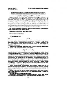
Figure 3.1: A multigraph with loops at v3 , v6 , and v11 , three parallel arcs (v2 , v4 ), two parallel arcs (v8 , v10 ), as well as anti-parallel arcs {(v4 , v5 ) , (v5 , v4 )}, {(v8 , v10 ) , (v10 , v8 )}, and {(v9 , v11 ) , (v11 , v9 )}.

a graph has parallel or anti-parallel arcs, if one of its arcs has parallel or anti-parallel arcs, respectively. A graph with loops, parallel, or anti-parallel arcs is called a multigraph. Otherwise, the graph is said to be simple. In the latter case, it suffices to define A as a simple set, i. e. , A ⊂ V × V . Figure 3.1 provides an example of a multigraph that will serve as a running example for the remainder of this chapter.

A graph G′ = (V ′ , A′ ) is a subgraph of G, denoted by G′ ⊆ G, if V ′ ⊆ V and A′ ⊆ A

as well as A′ ⊆∗ V ′ × V ′ . A subgraph G′ is spanning if V ′ = V . For a set of vertices X ⊆ V , the induced subgraph GX is the subgraph of G with vertex set X and arc set

(UX , mX ), where UX = {(u, v) ∈ U | u ∈ X ∧ v ∈ X} and ∀a ∈ UX : mX (a) = m(a). Using a set of arcs Y , we define the spanning subgraph G⏐Y of G that is restricted to Y as ⏐

G⏐Y = (V, A ∩ Y ). ⏐

A tournament is a simple graph G = (V, A) such that for each distinct pair of vertices

u, v ∈ V , u ̸= v, exactly one of the arcs (u, v) and (v, u) is in A. A graph is bipartite if its vertex set V can be partitioned into two sets V ′ ∪˙ V ′′ = V such that for all arcs (u, v) ∈ A, either u ∈ V ′ and v ∈ V ′′ or u ∈ V ′′ and v ∈ V ′ . A bipartite tournament is a simple bipartite graph G = (V ′ ∪˙ V ′′ , A) with exactly one of (u, v) and (v, u) in A for each pair of vertices u, v such that u ∈ V ′ and v ∈ V ′′ .

3.2.2 Vertex Degrees For a vertex v ∈ V , we denote by N+ (v) the simple set of vertices that v has an outgoing arc to, i. e. , N+ (v) = {u ∈ V | (v, u) ∈ U }. Likewise, N− (v) denotes the simple set of vertices that v has an incoming arc from, i. e. , N− (v) = {u ∈ V | (u, v) ∈ U }. The

outdegree d+ (v) of v is defined as the number of arcs that are outgoing from v, also

40


counting parallel arcs, i. e. , d+ (v) = indegree, i. e. , d− (v) =

u∈N+ (v) m((v, u)).

∑

u∈N− (v) m((u, v)).

∑

Equivalently, d− (v) denotes v’s

Finally, the (total) degree d(v) of v is defined

as d(v) = d (v) + d (v) and the delta degree δ(v) as δ(v) = d+ (v) − d− (v). Note that for +

every graph,

−

∑

v∈V

δ(v) =

∑

v∈V

d+ (v) −

∑

v∈V

d− (v) = 0.

A vertex v is called a source if d+ (v) ≥ 1 and d− (v) = 0 and a sink if d+ (v) = 0 and

d− (v) ≥ 1. In case d(v) = 0, v is said to be isolated. The maximum degree of a vertex in a graph is denoted by ∆G , i. e. , ∆G = maxv∈V d(v).

A graph G is k-regular, if ∀v ∈ V : d(v) = k and k-subregular, if ∀v ∈ V : d(v) ≤ k,

or equivalently, ∆G = k. For k = 3, we also refer to such a graph as cubic or subcubic, respectively. For k = 4, the terms quartic and subquartic are used as an alternative. In case of k = 5, a graph is called quintic or subquintic, respectively.

3.2.3 Paths, Cycles, and Walks A path P of length k is an alternating sequence of k + 1 vertices and k connecting arcs P = ⟨v0 , (v0 , v1 ) , v1 , (v1 , v2 ) , v2 , . . . , vk−1 , (vk−1 , vk ) , vk ⟩. In case no ambiguity arises, we may also specify a path by giving only either its vertices or arcs. As a short form, we write v0 ⇝ vk to denote an unspecified path from v0 to vk . A path is simple, if it does not include a vertex more than once. Let VP = {v0 , v1 , . . . , vk } be the set of vertices of

P and AP = {(v0 , v1 ) , (v1 , v2 ) , . . . , (vk−1 , vk )} the set of arcs of P. With a slight abuse of notation, we write v ∈ P for a vertex v ∈ V to express that v ∈ VP , and a ∈ P for an arc a ∈ A to express that a ∈ AP .

A path P′ is a subpath of a path P = ⟨v0 , (v0 , v1 ), v1 , (v1 , v2 ), v2 , . . . , vk−1 , (vk−1 , vk ), vk ⟩,

if P′ = ⟨vi , (vi , vi+1 ), vi+1 , . . . , vj−1 , (vj−1 , vj ), vj ⟩, for some i, j with 0 ≤ i ≤ j ≤ k, i. e. , P′ is a continuous subsequence of vertices and arcs of P.

Two paths P and P′ are vertex-disjoint if they do not share a common vertex. Likewise, P and P′ are arc-disjoint, if they do not share a common arc. Every vertex-disjoint pair of paths is also arc-disjoint. A cycle C of length k is a path of length k where the first and the last vertex coincide, i. e. , v0 = vk . For a cycle to be simple, all vertices apart from v0 , vk must be distinct. Whenever a graph contains a cycle C that is not simple, it also contains a simple cycle C′ that consists of the shortest subpath in C that begins and ends at the same vertex. The notion of vertex- and arc-disjointness is transferred from paths to cycles analogously, i. e. , two cycles C and C′ are vertex-disjoint (arc-disjoint) if no vertex (arc) is contained in both C and C′ .

41

3.2 General Graph Theory Note that paths and cycles of length k = 1 are single arcs and loops, respectively.

Similar to a path, a walk W of length k is an alternating sequence of k + 1 vertices and k arcs W = ⟨v0 , a{v0 ,v1 } , v1 , a{v1 ,v2 } , v2 , . . . , vk−1 , a{vk−1 ,vk } , vk ⟩ with the vital difference that

a{vi ,vj } may either be the arc (vi , vj ) or its reverse, i. e. , (vj , vi ). Informally, a walk is a path where the arcs’ directions are ignored. Consequently, every path is also a walk, but not vice versa.

3.2.4 Connectivity and Acyclicity A graph G is said to be connected, if there is a walk from u to v for every pair of vertices u, v ∈ V . G is said to be k-vertex-connected or simply k-connected, if n > k and for any subset of at most k − 1 vertices V ′ ⊊ V , GV \V ′ is connected, i. e. , the removal of at most

k−1 arbitrary vertices does not disconnect G. A 2-connected graph is synonymously also called biconnected. A connected component of a graph is a maximal connected subgraph, i. e. , for X ⊆ V , GX is a connected component if GX is connected if there is no superset X ′ ⊋ X such that GX ′ is connected. Analogously, a biconnected component or block of a

graph is a maximal biconnected subgraph. A vertex v is called a cut vertex, if GV \{v} has more connected components than G. In particular, a graph is biconnected if and only if it does not have a cut vertex. The definition implies that every cut vertex of a graph is part of at least two blocks. The block-cut tree of a graph G is an unrooted tree T whose nodes each represent either a block or a cut vertex of G. Two nodes of T are adjacent if

and only if one of them represents a block, the other a cut vertex, and the block contains the cut vertex. The graph depicted in Figure 3.1, e. g. , is not biconnected due to the presence of the (only) cut vertex v10 . It contains two blocks: one consisting of all vertices vi with 0 ≤ i ≤ 10, and second consisting of all vertices vj with 10 ≤ j ≤ 13. Observe that v10 is contained in both blocks. The block-cut tree of this example graph thus consists of three nodes representing two blocks and one cut vertex. For two vertices u, v of a graph G, v is said to be reachable from u if there is a path u ⇝ v in G. The vertices u and v are called strongly connected, if they are mutually reachable, i. e. , there are paths u ⇝ v and v ⇝ u in G. By transferring this definition to the whole graph, we obtain that a graph is strongly connected, if there is a path between each ordered pair of vertices. A strongly connected component, SCC for short, of a graph is a strongly connected subgraph that is maximal with respect to its vertex set. Formally, the property of being

42


v13

σ2 v1

v3

v5

v12 v10

σ0 v4

v0

v2

v8

v6 σ1

v7

v11

v9

σ5

σ4

σ3

Figure 3.2: Strongly connected components of the example graph.

σ0

σ2

σ5

σ1

σ3

σ4

Figure 3.3: The condensation of the example graph.

strongly connected defines an equivalence relation on the set of vertices such that each equivalence class corresponds to the vertex set of exactly one SCC. This also implies that any two vertices vi , vj of a cycle C are strongly connected, as C can be split into two paths vi ⇝ vj and vj ⇝ vi . Therefore, for every cycle in G, its vertices and arcs must be part of the same SCC. Figure 3.2 shows the SCCs of the example graph. In general, the number of SCCs in a graph may range between 1 and n. In the former case, the graph itself is strongly connected, while in the latter, every SCC consists of a single vertex only. If so, the graph does not contain a cycle of length k > 1. A graph is said to be acyclic, if it does not contain a cycle of length k > 0. In consequence, every loop-free graph with n SCCs is acyclic. Contracting each SCC of G to a single vertex always yields an acyclic graph that is called the condensation of G. See Figure 3.3 for the condensation of the example graph. In an acyclic graph, the reachability relation defines a partial order on the set of its vertices. Every linear extension of this relation (i. e. , to a total order) corresponds to a topological sorting of the acyclic graph. A topological sorting of G = (V, A) is a bijective mapping ξ : V → {0, . . . , n − 1} that assigns a topsort number ξ(v) to every vertex v such

43

3.3 Feedback Arc Sets and Linear Orderings

σ1

σ0

σ5

σ2

σ3

σ4

σ5

σ1

σ0

σ2

σ3

σ4

Figure 3.4: Two possible topological sortings of the condensed example graph. that ∀ (u, v) ∈ A : ξ(u) < ξ(v). Descriptively, every arc must point from a vertex with

a lower topsort number to a vertex with a higher topsort number. A graph is acyclic if and only if it can be sorted topologically. Just as there may be a number of different linear extensions to a partial order, there may be equally many topological sortings of an acyclic graph. For illustration, Figure 3.4 shows two possible topological sortings of the condensed example graph. Computing a topological sorting and inherently checking whether a graph is acyclic can be accomplished in time O(n + m) by repeatedly removing a source v from the graph

and assigning it the topsort number ξ(v) in increasing order. We refer to the algorithm that returns a topological sorting of an acyclic graph G as TopSort(G) . The strongly connected components of a graph can also be retrieved in time O(n + m)

using, e. g. , Tarjan’s algorithm [Tar72], which is based on depth-first search. At the same time, the graph’s condensation may be constructed.

3.3 Feedback Arc Sets and Linear Orderings This section is to introduce notation that relates especially to the mathematical handling of feedback arc sets and linear orderings.

3.3.1 Feedback Arc Sets A feedback arc set B, sometimes also called a cycle cover, for a graph G = (V, A) is a set

of arcs B ⊆ A such that the subgraph restricted to A \ B is acyclic. The set F = A \ B is

referred to as the acyclic arc set of G with respect to B and the subgraph restricted to F, G⏐F , as the according acyclic subgraph. ⏐

Given a set of arcs B ⊆ A, we say that B is feasible, if it forms a valid feedback arc set.

In conformance with the definitions in Section 3.1, a feedback arc set is called minimal, if no arc can be removed from it such that it remains feasible. Analogously, a feedback arc

44


v10

v8

v10

v11

v8

v9

v10

v11

v8

v9 (a)

v11

v9 (b)

(c)

Figure 3.5: A feasible feedback arc set (a), a minimal feedback arc set (b), and an optimal (minimum) feedback arc set (c) for the subgraph σ5 , highlighted by dotted red arcs. set is minimum, if its cardinality is minimum among all feedback arc sets of G. In this case, the feedback arc set is also said to be optimal. Figure 3.5 shows three different feedback arc sets for the strongly connected subgraph σ5 of the example graph. In the first example, Figure 3.5(a), one of the arcs (v8 , v9 ), (v9 , v10 ), or (v10 , v11 ) could be removed from the feedback arc set while still maintaining feasibility. This is not the case for the feedback arc set depicted in Figure 3.5(b), however, its cardinality is not minimum among all feedback arc sets, as Figure 3.5(c) testifies. In fact, the last figure shows an optimal feedback arc set. We denote the cardinality of an optimal feedback arc set by τG or simply τ , if no ambiguity arises. If B is an (optimal) feedback arc set for a graph G, then B R is an (optimal) feedback

arc set for the reverse graph GR . In particular, this implies that τG = τGR .

The optimal feedback arc set is the empty set if and only if the graph is acyclic.

3.3.2 Linear Orderings A linear ordering πG of G = (V, A) is a bijective mapping πG : V → {0, . . . , n − 1} that

assigns a unique LO position πG (v) to every vertex v ∈ V . An arc (u, v) is called forward, if πG (u) < πG (v), and otherwise backward. Two vertices u, v ∈ V are said to be consecutive

with respect to πG , if their LO positions differ by exactly one, i. e. , |πG (u) − πG (v)| = 1. More generally, a set X ⊆ V of vertices is called consecutive with respect to πG , if maxu,v∈X |πG (u) − πG (v)| = |X| − 1.

Linear orderings are usually visualized by aligning the vertices horizontally and

sorting them according to their LO positions in increasing order from left to right. Forward arcs are then drawn as arches above or on the same level as the vertices, while backward arcs appear below it. We denote by FπG and BπG the set of arcs that are

45


v11

v10

v9

v8

v11

v9

v10

v8

v8

(a)

v9

v10

v11

(b)

(c)

Figure 3.6: Linear orderings of the subgraph σ5 , such that the backward arcs in (a), (b), and (c) each correspond to the respective feedback arc set shown in Figure 3.5. v0

v1

v2

Figure 3.7: A feasible feedback arc set without corresponding linear ordering. classified by πG as forward and backward, respectively. We omit the subscript and simply write π instead of πG if the graph it refers to is clear from the context. In fact, linear orderings bear resemblance to topological sortings, but with the important distinction that the latter do not allow for backward arcs. If we consider the subgraph restricted to the forward arcs, however, then π indeed is a topological sorting of this subgraph. Consequently, π defines an acyclic subgraph G⏐Fπ of G along with a ⏐

feedback arc set, which corresponds exactly to the set of arcs classified as backward, Bπ . Note that if we consider instead the subgraph restricted to the backward arcs excluding loops, then the reversal of π again is a topological sorting. Hence, G⏐Bπ may contain ⏐

cycles of length at most one. We say that a vertex v ∈ V is a pseudosource with respect to a linear ordering π if v is a source in G⏐Fπ . Analogously, a vertex v ∈ V is called a ⏐

pseudosink with respect to a linear ordering π if v is a sink in G⏐Fπ . ⏐

Figure 3.6 uses the subgraph σ5 of the example graph again and shows three linear orderings. The set of backward arcs in each of them corresponds to the feedback arc set depicted in the respective subfigure of Figure 3.5. A linear ordering uniquely identifies a feedback arc set Bπ and an acyclic arc set Fπ ,

whereas the opposite does not hold true in general. On the contrary, every topological sorting of G⏐Fπ yields a linear ordering π ′ such that Bπ′ ⊆ Bπ , i. e. , the topological sorting ⏐

may “accidentally” have classified arcs of Bπ as forward. This implies that, first, there

may be multiple linear orderings that define the same feedback arc set and, second, not every feedback arc set B has a corresponding linear ordering π such that B = Bπ . For a

46


v10

v8

v11 v11

v10

v9

v8

v9 (a)

(b)

Figure 3.8: Construction of linear ordering that corresponds exactly to the feedback arc set depicted in Figure 3.5(a): reversal of non-loop backward arcs (a) and topological sorting (b). For illustration, reversed backward arcs are drawn below the vertex level. graph consisting only of a cycle of length k > 1, for example, such as the graph shown in Figure 3.7, the set of all arcs is feasible, but we have already argued in the paragraph before last that for any linear ordering π, the subgraph G⏐Bπ must be acyclic except for ⏐

loops. If this requirement is met, however, a construction of π is possible, which is also exemplified in Figure 3.8. Observation If there is an acyclic arc set F ⊆ A of a graph G = (V, A) and the set B = A \ F

does not contain a cycle of length k ≥ 2, a corresponding linear ordering π can

be obtained such that B = Bπ by topologically sorting the graph that consists of G⏐F plus the reverse of each arc in B that is not a loop. ⏐

The characteristic of inducing the same set of backward arcs yields an equivalence relation ∼B on the set of linear orderings of a graph. The equivalence class of π hence is the set containing all linear orderings π ′ that induce exactly the same set of backward arcs as π, i. e. , [π]∼B = {π ′ | Bπ′ = Bπ }. Using the above observation, [π]∼B can be constructed explicitly by compiling all topological sortings.

To ease notation, we define |π| = |Bπ |. We also adopt the terminology from sets and

say that a linear ordering π is optimal, if its induced feedback arc set Bπ is. To express that

∗ | = τ . Note a linear ordering π is optimal, we denote it by π ∗ , i. e. , we always have |πG G

that all linear orderings in the equivalence class [π ∗ ]∼B of an optimal linear ordering π ∗ are also optimal.

For a linear ordering π, we define the reverse linear ordering π R as π R : V → {0, . . . , n − 1}

where π R (v) = n − 1 − π(v) for every vertex v ∈ V . This definition complies well with

the definition of the reverse graph: If πG is a linear ordering of G, then πG R forms the

47


corresponding linear ordering for GR such that BπG R equals the set of backward arcs

induced by πG R on GR , i. e. , BπG R = BπG R . In particular, this implies that πG is an optimal linear ordering of G if and only if πG R is an optimal linear ordering of GR . Note that also the reversion of a linear ordering is an involution, i. e. , πG R R = πG . Finally, we simplify Bπ and Fπ to B and F, respectively, if the linear ordering that

these sets are obtained from is unambiguous. In the context of a linear ordering π, B and F always refer to Bπ and Fπ .

3.3.3 Forward Paths and Layouts Given a linear ordering π of a graph G = (V, A), a path P is called forward path if every arc in P is forward. For every vertex v ∈ V , π defines four (multi-)sets of arcs: F − (v), F + (v), B − (v),

B + (v), which contain the incoming forward, outgoing forward, incoming backward, and outgoing backward arcs of v according to π. Additionally, we use F(v) = F − (v) ∪ F + (v) and B(v) = B − (v) ∪ B + (v) if we do not want to distinguish between incoming

and outgoing arcs. We denote the cardinalities by f − (v) = |F − (v)|, f + (v) = |F + (v)|, b− (v) = |B − (v)|, and b+ (v) = |B + (v)|. Analogously, we set f(v) = f − (v) + f + (v) =

|F(v)|, and b(v) = b− (v) + b+ (v) = |B(v)| to express the total number of forward

and backward arcs incident to v, respectively. For ease of notation, let φ[X], for φ ∈

{F − , F + , B − , B + , f − , f + , b− , b+ }, be the canonical extension of the function φ to sets of

elements, e. g. , F − [X] =

induces a layout L : V →

(f − (v), f + (v), b− (v), b+ (v)).

v∈X F (v) and f N40 such that for

⨄

−

−

[X] = |F − [X]|. The linear ordering π

each vertex v ∈ V , L(v) is the 4-tuple

Note that if we consider the reverse graph GR along with the reverse linear ordering π R , then for every vertex v ∈ V , its incoming forward arcs according to π in G correspond to

its outgoing forward arcs according to π R in GR and its outgoing forward arcs according to π in G correspond to its incoming forward arcs according to π R in GR . Likewise, its incoming backward arcs according to π in G correspond to its outgoing backward arcs according to π R in GR and its outgoing backward arcs according to π in G correspond to its incoming backward arcs according to π R in GR . In order to improve comprehensibility, we use pictograms that visualize the layout as a shorthand notation for the 4-tuples, depending on the degree of accuracy needed. In a pictogram, a simple arc ( ) always signifies exactly one arc, whereas an arc with a double shaft ( ) serves as a representative for a set of arcs. We use a dotted version

48


( ), if the represented arc set may be empty, otherwise, the lines are drawn solid. In the latter two cases, identical colors and drawing styles of two double shaft arcs indicate identical arc set cardinalities, provided that they are incident to the same vertex. (We would run out of drawing styles if we also kept this invariant across different vertices.) The pictogram

, for instance, represents a vertex v with L(v) = (i, j, k, l), where

i ≥ 0, j = k + 1, k ≥ 1, and l = 2.

3.4 Preprocessing and Default Assumptions The L INEAR O RDERING problem consists in finding an optimal linear ordering π ∗ of a graph G. Prior to tackling this task, there are a few preprocessing steps which can be taken to facilitate the handling of G. In this section, we will introduce them briefly and see how they enable us to set up some default assumptions on the input graphs. Unless indicated otherwise, the restrictions listed here shall be effective for the remainder of this thesis.

3.4.1 Loops and Anti-Parallel Arcs Consider a graph G = (V, A) as input to the L INEAR O RDERING problem. By the definition of a linear ordering, a loop is always classified as a backward arc. Let l denote the number of loops of the input graph G and let G′ be the subgraph of G that contains all arcs but loops. Then, every linear ordering of G′ is also a linear ordering of G and vice versa, whose set of backward arcs differ by exactly the l loops. The same applies to pairs of anti-parallel arcs. Let {(u, v) , (v, u)} ⊆ A be such a pair

and let G′ be the subgraph of G restricted to A \ {(u, v) , (v, u)}. Note that parallel arcs

of (u, v) or (v, u), if existent, remain in G′ . Again, every linear ordering of G′ is also a linear ordering of G and vice versa, whose set of backward arcs differ by exactly 1: In case that u has a smaller LO position than v, G has (v, u) as an additional backward arc, otherwise, the additional backward arc is (u, v). In consequence, loops and anti-parallel arcs can be deemed irrelevant for the construction of a linear ordering. We can therefore remove all loops from the input graph as well as anti-parallel arcs pairwisely and proceed with the resulting graph, which is simple up to parallel arcs. After the construction of the linear ordering, these arcs are reinserted. The manipulation of graphs and their effects on the L INEAR O RDERING problem are also discussed in more detail in Section 4.10.1.

49

3.4 Preprocessing and Default Assumptions

v13 v1

v3

v5

v10

v4

v0

v2

v6

v12

v8

v7

v11

v9

Figure 3.9: The example graph of the previous section after the removal of loops and anti-parallel arcs. In the following, we confine ourselves to considering only graphs without loops and anti-parallel arcs: Assumption 3.1 The input graph is free of loops and anti-parallel arcs. The result of the application of the preprocessing steps described above to the example graph of the previous section is shown in Figure 3.9.

3.4.2 Strong Connectivity Consider now a graph G = (V, A) that is not strongly connected. In Section 3.2.4, we have already seen that no cycle of the graph can contain vertices of different strongly connected components. It therefore suffices to solve the problem on the SCCs separately and combine the results afterwards: Let σ0 , . . . , σk be the strongly connected components of G and let π0 , . . . , πk be linear orderings of them, respectively. Denote by B0 , . . . , Bk the according induced sets of backward arcs. Then, B =

⋃

0≤i≤l

Bi is a feedback arc set of G with |B| =

∑

0≤i≤k

|Bi |.

⏐ A corresponding linear ordering π of G can be obtained by either sorting G⏐F topolog-

ically (cf. Section 3.3) or by “concatenating” the linear orderings of the SCCs in the order of the topological sorting of the condensation of G, i. e. , if ξ is a topological sorting of the condensation of G and u, v are two vertices of G, then π(u) < π(v) if and only if either u and v are vertices of the same SCC σi and πi (u) < πi (v) or u belongs to SCC σi and v belongs to SCC σj , i ̸= j, and ξ(σi ) < ξ(σj ). Note that for the sake of simplicity, the

SCCs and the vertices of the condensation graph have been identified in this definition. This allows us to impose the following restriction:

50


v13

σ6 v1

v3

σ0

v5 σ2 v4

v0

v12 v10

v2

v8

v6 σ1

v7 σ3

v11

v9

σ5

σ4

Figure 3.10: The strongly connected components of the graph depicted in Figure 3.9.

Assumption 3.2 The input graph is always strongly connected. For illustration, Figure 3.10 depicts the strongly connected components of the graph shown in Figure 3.9, i. e. , the example graph of the previous section after the removal of loops and anti-parallel arcs.

3.4.3 Biconnectivity Finally, consider the case that G = (V, A) is strongly connected, but not biconnected. The following fact is commonly known (cf. [Sta90]): Proposition 3.1 A set of arcs B ⊆ A is a feedback arc set for a graph G = (V, A) if and only if B=

⋃

i Bi

such that Bi is a feedback arc set of βi , for every block βi of G.

As this may not be entirely obvious at first glance, we provide a short proof here. Proof. Let β0 , . . . , βk denote the blocks of G and let T be the block-cut tree of G. Consider

two vertices u, v ∈ V that are not cut vertices and contained in blocks βu and βv , respectively, such that βu ̸= βv . As G is strongly connected, there must be paths P = u ⇝ v and P′ = v ⇝ u in G. Both paths contain all cut vertices X on the path from

βu to βv in T . Let C denote the cycle consisting of P and P′ . In this case, C contains all

vertices in X at least twice, i. e. , C is not simple. Instead, C consists of a set of simple

cycles formed by the subpaths between two cut vertices. The vertices of every such simple cycle are subsequently contained in a common block of G. Furthermore, C is


51

covered by a feedback arc set if and only if every cycle of this set of simple cycles is covered. Hence, it suffices to solve the L INEAR O RDERING separately on each block and combine the result afterwards, which allows us assume: Assumption 3.3 The input graph is biconnected. Let β0 , . . . , βk again denote the blocks of G and let π0 , . . . , πk be their respective linear orderings. A linear ordering π of the graph G can be obtained by sorting the acyclic subgraph G⏐F that results from removing all arcs that have been classified as backward ⏐

by one of π0 , . . . , πk topologically, as Proposition 3.1 immediately suggests. Alternatively, π can be constructed directly from the π0 , . . . , πk as follows: Traverse the block-cut tree T of G by a depth-first search to obtain a preordering of the blocks and sort the linear orderings of the blocks according to this preorder. For simplicity, assume that π0 , . . . , πk

is already such an ordering. We incrementally construct a combined linear ordering: Let π (0) = π0 . For 0 < i ≤ k, let vi denote the only common vertex of πi and π (i−1) .

This vertex must be a cut vertex, as it is part of at least two blocks, and, as T is a tree, there can only be one such vertex. Construct π (i) from π (i−1) by replacing vi in π (i−1)

with the linear ordering πi . More formally, for two distinct vertices u ̸= w contained in

one of the blocks β0 , . . . , βi , π (i) (u) < π (i) (w) if and only if either both are contained in βi and πi (u) < πi (w), or both are not contained in βi and π (i−1) (u) < π (i−1) (w), or u is contained in βi , w is not contained in βi , and π (i−1) (vi ) < π (i−1) (w), or u is not contained in βi , w is contained in βi , and π (i−1) (u) < π (i−1) (vi ). Then, π = π (k) is a linear ordering of G that conforms with every linear ordering πi , 0 ≤ i ≤ k.

With respect to the aim of using all assumptions concurrently, let us briefly address the

question of whether a block of a strongly connected graph is again strongly connected. Proposition 3.2 Every block β of a strongly connected graph G is itself strongly connected.

Proof. Let T be the block-cut tree of G and let u, v be two vertices of the same block β of

T . As G is strongly connected, there is a path P = u ⇝ v in G. If P contains only vertices of β, P is also a path in β. Suppose P contains a vertex that does not belong to β. In

this case, P must also pass through at least one cut vertex. Let w be the first cut vertex

52


v10

v8

v11 v8

β0

v9

v10

v11

v9 (a)

(b)

Figure 3.11: The block β0 of σ5 along with an (optimal) linear ordering.

v13 β1

v12

v12

v10

v10

(a)

v13 (b)

Figure 3.12: The block β1 of σ5 along with an (optimal) linear ordering. encountered on a traversal of P. Then, w is contained in β and P leaves β at w. However, P must end at v, which is also contained in β and, as T is a tree and w is a cut vertex, P

must enter β again at w. Subsequently, β contains a path u ⇝ w as well as a path w ⇝ v. Hence, β contains a path u ⇝ v for every pair of vertices u, v, which implies that β is strongly connected. We can thus continue the preprocessing of the input graph after the removal of loops and pairs of anti-parallel arcs as well as the partition into strongly connected components by simply splitting these SCCs up into blocks. The strongly connected components of the example graph, as visualized in Figure 3.10 are all biconnected except for σ5 , which has a cut vertex v10 . Figure 3.11 and Figure 3.12 show the two blocks of σ5 along with an optimal linear ordering for each block. The block-cut tree of σ5 is depicted in Figure 3.13(a). The linear ordering for σ5 obtained using the procedure described above is given in Figure 3.13(b).

v10 β0

v8

v9

v12

v10

v13

v11

β1 (a)

(b)

Figure 3.13: The block-cut tree of σ5 and the linear ordering constructed from those of β0 and β1 .

53


σ1

σ0

σ5

σ2

σ3

σ4

σ6

Figure 3.14: A topological sorting of the SCCs depicted in Figure 3.10.

v2

v0

v1

v3

v8

v9

v12

v10

v13

v11

v4

v6

v7

v5

Figure 3.15: An (optimal) linear ordering of the graph depicted in Figure 3.10, obtained by concatenating the linear orderings of the SCCs in the order of the topological sorting as shown in Figure 3.14.

v2

v0

v1

v3

v8

v9

v12

v10

v13

v11

v4

v6

v7

v5

Figure 3.16: An optimal linear ordering of the example graph after the reinsertion of loops and pairs of anti-parallel arcs. The linear ordering corresponds to that depicted in Figure 3.15.

54


In order to finish the example, we next obtain a topological sorting of the condensation of the graph shown in Figure 3.10, which is depicted in Figure 3.14. Afterwards, the separately computed, here even optimal, linear orderings of the SCCs can be “concatenated” in the order of the topological sorting (cf. Figure 3.15). Finally, the loops and anti-parallel arcs are reinserted into the graph, thus leading to a linear ordering of the original input graph. Figure 3.16 provides the optimal linear ordering of the example graph that has arisen from these steps.

4

Properties of Optimal Linear Orderings: A Microscopic View

Finding the absolutely best solution to a problem is often time consuming, and, if the instance is big enough, at times even impossible. In this chapter, we specifically study optimal solutions to the L INEAR O RDERING problem to gain more insight into their structure. In doing so, we apply a kind of microscopic view with the emphasis being placed primarily on single arcs and vertices, thus opposing more “macroscopic” approaches that operate on higher abstraction levels. Whereas this limitation might appear disadvantageous at first sight, it turns out to be powerful in sum due to synergy effects. We benefit algorithmically in two respects: First, approximation algorithms and heuristics can be improved to yield better solutions while still running in polynomial time. In the course of this chapter, algorithms are developed that monotonically improve a given linear ordering. Second, exact algorithms can take advantage of these findings and be sped up. A third aspect consists in the ability to prove new bounds on the cardinality of an optimal solution for different kinds of graphs. As a consequence, the contents provided here form the basis for all subsequent chapters.

4.1 General Framework A solution to a problem is optimal if and only if it is at least as good as every other solution. This is the common definition for optimality. As L INEAR O RDERING is a minimization problem, the part “is as good as” translates to “induces at most as many backward arcs as” here. In order to obtain a more formal definition, we introduce a predicate Opt which expresses whether a linear ordering π is optimal, i. e. , Opt(π) =

56


true, or not, i. e. , Opt(π) = false or ¬Opt(π) = true. Then, we can express optimality as follows:

Opt(π) ⇔ ∀π ′ : |π| ≤ ⏐π ′ ⏐ ⏐ ⏐

As mentioned at the beginning, finding such a solution for N P-hard optimization

problems such as LO and FAS is in any case resource consuming and sometimes impossible in practice. Instead, one tries to find good solutions, where “good” may be interpreted in different ways. A “good” solution may, e. g. , be one that is provably close to the optimum, with the downside that something about the optimal solution must be known. A different approach consists in optimizing a given solution as far as possible. Optimality is unquestionably a very ambitious property for a linear ordering to achieve. In the following sections, we therefore establish a more accessible set of properties with the characteristic that if a linear ordering disrespects one of them, it is not optimal and can be improved in a prespecified way. A special class of such properties consists in those who require a coupling with another property such that the compliance of a linear ordering depends on the choice of the partner. We call such properties meta-properties and address a selection of them in the last section of this chapter. Just as Opt indicates whether or not a linear ordering is optimal, we define a predicate for every introduced property that can be established efficiently and that is not a metaproperty. Furthermore, we define a set Ψ that encompasses all these predicates. The “superpredicate” Ψopt then expresses that a linear ordering has all properties defined by the predicates in Ψ: Ψopt (π) ⇔ ∀ψ ∈ Ψ : ψ(π) We call a linear ordering π Ψ-optimal if and only if Ψopt (π) = true. As a reminder, we point out that π ∗ always denotes an optimal linear ordering, i. e. , Opt(π ∗ ) is always true (cf. Section 3.3). In this chapter, we prove the following two theorems: Theorem 4.1 For every linear ordering π holds: Opt(π) ⇒ Ψopt (π). A characteristic of the properties in Ψ is that all can be established concurrently and in polynomial time, which allows us to implement a Ψopt -algorithm for L INEAR O RDERING.

57

4.1 General Framework

Theorem 4.2 2

1

There is an O(n · m2 · min{n 3 , m 2 })-time algorithm that constructs a Ψ-optimal linear ordering π.

In the individual sections of the chapter, we will introduce each property separately, prove its validity for optimal linear orderings, and, where applicable, provide a propertyestablishing algorithm. A common feature of these algorithms is that they can be conveniently formulated by means of the routine Iterate (cf. Algorithm 4.1): Let E(G, π) be an algorithm that takes a graph G and a linear ordering π as input and returns π if it respects the respective property. Otherwise, it applies an improvement to π and returns this new linear ordering. Then, Iterate(G, π, E) establishes the property by calling E(G, π) until no further improvement is possible, i. e. , E ’s return value equals its argument π. Algorithm 4.1 Iterate Require: graph G, linear ordering π, property-enforcing routine E(G, π) Return: a linear ordering obtained from π that respects the property enforced by E(G, π) 1:

procedure Iterate(G, π, E)

2: 3: 4: 5:

π′ ← π repeat

π ← π′

π ′ ← E(G, π)

6:

until π = π ′

7:

return π

A crucial characteristic of every property-enforcing routine E(G, π) is that it never returns a linear ordering π ′ such that |π ′ | > |π|. This monotonicity in combination

with the wrapper algorithm Iterate yields a local search heuristic for every routine E which employs a technique that is also known as hill climbing. In contrast to simulated annealing or tabu search, no worsening of the solution, even if only temporarily, can occur. The local search terminates as soon as E no longer modifies the linear ordering, i. e. , π = π ′ in the pseudocode. Prior to this, the linear ordering must have been improved in each call to the property-enforcing routine, i. e. , |π| decreases by at least one per loop

58


iteration. As 1 ≤ |π| ≤ m, this enables us to bound the running time of Iterate(G, π, E) depending on E as follows1 : Proposition 4.1 Iterate(G, π, E) runs in O(m) times the running time of E(G, π).

4.2 Algorithmic Setup In the current chapter, several algorithms are devised that construct and manipulate linear orderings. The data structures given in this section serve as a basis for future time complexity analyses. Along with these, two initialization algorithms are introduced that may be used as ingredients to other algorithms later.

4.2.1 Graphs We start with a suitable data structure to represent the input graph. Taking into account that the algorithms studied in the following sections construct or manipulate different linear orderings of the input graph, but not the graph itself, there is no need to attach great importance to the cost of vertex or arc additions and deletions. We are, however, interested in being able to efficiently obtain the vertices and arcs that are linked with a vertex. Furthermore, this thesis focuses especially on sparse graphs, hence, space complexity may be worth a consideration. For these reasons, we assume an adjacency list representation here, or, more precisely, an incidence list representation, i. e. , every vertex stores a list of incident incoming and outgoing arcs. For an efficient handling of parallel arcs in multigraphs, we assume that they are represented blockwisely in the incidence lists, such that the parallel copies of an arc can be skipped in O(1) in the traversal of an incidence list where required.

Additionally, every arc a knows its head and tail, which can be accessed by head(a) and tail(a) in constant time. Accessing the reverse of a graph does not cause more than constant overhead if only the roles of the lists of incoming and outgoing arcs at each vertex are swapped and heads are treated as tails and vice versa. We further maintain F and B as sets and additionally a flag attached to each arc

specifying whether this arc is classified as forward or backward according to the current 1

See also Section 4.2.5 for further remarks on an efficient implementation of Iterate.

59

4.2 Algorithmic Setup

linear ordering. Consequently, computing, e. g. , a topological sorting of an acyclic subgraph can be accomplished by ignoring all arcs with flag “backward”.

4.2.2 Linear Orderings There are essentially two possibilities of how a linear ordering can be implemented. Mathematically, it is modeled as a bijective function from the set of vertices V to the set of natural numbers ranging from 0 to n − 1. A data structure that comes relatively close

to this is the map, which is sometimes also called an associative array or a dictionary. A different approach consists in storing the actual ordering of the vertices in a linear data structure such as an array or a linked list. Both map and array share the advantage that the position of every vertex is stored explicitly (although in the case of an array, the mapping is technically from {0, . . . , n − 1} to V ). A drawback is, however, that even small changes to the relative ordering of the

vertices, e. g. , the movement of a single vertex to another position, requires up to O(n) updates. In case of a linked list, the situation is precisely the reverse. Here, such a move

operation can be accomplished in constant time, provided that the insertion position is known. In anticipation of the algorithms introduced in the following, we opt for a representation of a linear ordering as a doubly-linked list, which allows for an efficient traversal of the ordering in both directions. If needed, the exact position of a vertex within a linear ordering must be computed explicitly as shown in Section 4.2.4. Whenever the reverse of a linear ordering is accessed or modified by an algorithm, we assume that only a different interface is used, such that there is no additional overhead and changes to the reverse linear ordering also take effect directly on the original linear ordering.

4.2.3 Vertex Layouts A linear ordering induces a layout on each vertex. In Section 3.3.3, we introduced the sets F − (v), F + (v), B − (v), and B + (v) for a vertex v. As discussed earlier, we assume that the graph is represented using incidence lists. In order to also maintain these special sets, we add four additional incidence lists to each vertex. Every such list is sorted according to the positions of the tails in the current linear ordering for F − (v) and B − (v) and likewise according to the positions of the heads for F + (v) and B + (v), in each case in

60


Algorithm 4.2 Compute LO positions and forward/backward arc sets. Require: graph G = (V, A), linear ordering π Return: LO positions w. r. t. π, sets of backward and forward arcs B, F 1:

2: 3: 4: 5: 6: 7: 8: 9: 10: 11: 12:

procedure ComputePositionsAndArcSets(G, π) i←0

for all v in the order of π do π(v) ← i

▷ allow for fast “reverse lookup”: v has position i in π

i←i+1

F ← ∅; B ← ∅

for all (u, v) ∈ A do

if π(u) < π(v) then F ← F ∪ {(u, v)}

else

B ← B ∪ {(u, v)} return π, B, F

ascending order (with respect to the bijection π). We assume that the lists are represented as doubly-linked lists in any implementation. To denote the sorted list of arcs in F − (v) according to a linear ordering π, we introduce

a notation that is based on the definition of lists in Section 3.1 and write ⟨F − ⟩π (v). Likewise, we obtain ⟨F + ⟩π (v), ⟨B − ⟩π (v), and ⟨B + ⟩π (v) for F + (v), B − (v), and B + (v), respectively. If the linear ordering that these ordered lists refer to is clear from the context, the subscript may also be omitted.

4.2.4 Initializing the Data Structures Whereas we may readily assume that the graph is given with incidence lists, this is not a reasonable approach for the sorted lists introduced above. They depend heavily on a specific linear ordering, which is, by nature of this chapter, subject to change. The same applies to the exact position of a vertex within a linear ordering and the classification of arcs as forward or backward. Furthermore, algorithms may or may not make use of these additional structures. Therefore, it is desirable to be able to list their construction explicitly as a statement in pseudocode if needed. To this end, we provide two initializing routines, ComputePositionsAndArcSets(G, π) as well as ComputeLayoutLists(G, π), that take a graph G and a linear ordering π as

4.2 Algorithmic Setup

61

Algorithm 4.3 Compute vertex layouts. Require: graph G = (V, A), linear ordering π with precomputed LO positions Return: sorted layout lists ⟨F − ⟩, ⟨F + ⟩, ⟨B − ⟩, ⟨B + ⟩ 1:

procedure ComputeLayoutLists(G, π)

2: 3: 4: 5: 6: 7: 8: 9: 10: 11: 12: 13: 14:

for all v ∈ V do initialize ⟨F − ⟩ (v), ⟨F + ⟩ (v), ⟨B − ⟩ (v), ⟨B + ⟩ (v) with ⟨ ⟩

for all v in the order of π do

for all incoming arcs (u, v) of v do if π(u) < π(v) then ⟨F + ⟩ (u) ← ⟨F + ⟩ (u) ⋄ ⟨(u, v)⟩

else

⟨B + ⟩ (u) ← ⟨B + ⟩ (u) ⋄ ⟨(u, v)⟩

for all outgoing arcs (v, u) of v do if π(v) < π(u) then

⟨F − ⟩ (u) ← ⟨F − ⟩ (u) ⋄ ⟨(v, u)⟩

else

⟨B − ⟩ (u) ← ⟨B − ⟩ (u) ⋄ ⟨(v, u)⟩

return ⟨F − ⟩ , ⟨F + ⟩ , ⟨B − ⟩ , ⟨B + ⟩

input and perform these tasks. Algorithm 4.2 and Algorithm 4.3 show their respective details. We are able to identify two separate blocks in the listing of ComputePositionsAndArcSets: In lines 3–5, the algorithm iterates over all vertices in the order of their appearance within π. Concurrently, it maintains a counter variable i, which in each iteration corresponds to the position of the current vertex. For every vertex, the value of i is stored explicitly as an attribute. Next, in lines 7–11, the previously computed vertex positions are used to construct the sets F and B. ComputeLayoutLists starts by initializing the sorted lists ⟨F − ⟩ (v), ⟨F + ⟩ (v), ⟨B − ⟩ (v),

and ⟨B + ⟩ (v) with empty lists. In the loop spanning lines 3–13, the algorithm again

iterates over all vertices in the order they appear in π. For every vertex v, first all incoming arcs are considered. Let (u, v) be such an arc. If (u, v) is forward, then at the arc’s tail, u, (u, v) must be added to the end of u’s sorted list of outgoing forward arcs: The heads of all outgoing forward arcs of u that are not in the list yet must have a greater position in π than v, due to the fact that the algorithm iterates over the vertices

62


in the order of π. The same argument applies if (u, v) is backward, and likewise for all outgoing arcs of v. Lemma 4.1 The initialization routines ComputePositionsAndArcSets(G, π) and ComputeLayoutLists(G, π) run in time O(m) each.

Proof. Consider Algorithm 4.2 first. The first block, lines 3–5, iterates over all vertices of V . For each vertex, storing its position and incrementing the counter variable i can be accomplished constant time. Hence, the first block requires O(n) steps. The second block, lines 7–11, consists in iterating over all arcs of the graph, each time comparing two previously computed values and adding an arc to either F or B. For every arc, this can be done in constant time, so the running time of the second block is in O(m).

Consider now Algorithm 4.3 and assume that the linear ordering π is already equipped

with precomputed LO positions. The initialization with empty lists requires O(n) time. The remainder of the listing contains three nested loops. The outer loop iterates again

over all vertices. In its body, there are two more loops that iterate over the incoming and outgoing arcs, respectively, of the current vertex v. The body of every inner loop consists in querying the LO positions of an arc’s end vertices and appending the arc to the end of a list, both of which can be accomplished in constant time if the LO positions have been precomputed. The running time of the inner loops is therefore in O(d− (v)) and O(d+ (v)), respectively. Consequently, this block requires

∑

v∈V

d− (v) + d+ (v) = 2m

steps, which is in O(m).

In conclusion, with n ∈ O(m) due to G being strongly connected, the running time of

both ComputePositionsAndArcSets(G, π) and ComputeLayoutLists(G, π) is in O(m).

We stipulate that every algorithm that needs to access these additional structures is required to call the routines ComputePositionsAndArcSets and, if necessary, ComputeLayoutLists prior to querying them. After manipulating a linear ordering, it is the algorithm’s obligation to update the structures accordingly if it requires further access to them.

63

4.3 Nesting Property

4.2.5 General Remarks All algorithms presented in this chapter adhere to the concept of referential transparency, i. e. , calling a function or an algorithm with the same parameters will always produce the same result and there are no side-effects. For this reason, a property-enforcing routine E, e. g. , explicitly returns a linear ordering. In a faithful implementation in real code, this may result in additional overhead for copying the linear orderings back and forth and checking explicitly whether the linear ordering has actually been changed by E requires another O(n) steps. By waiving referential transparency and modifying the linear

ordering passed as argument directly or an intelligent copy-on-write implementation, these expenses can be saved. To avoid fundamental misconception of the presented algorithms, however, we stick to referential transparency in pseudocode, but assume an efficient realization for the runtime analyses. This is to apply to all algorithms, functions, and (sub-) routines used in this chapter. As noted before, we also assume that accessing the reverse of a graph or linear ordering is only a change of the interface and thus produces no additional overhead.

4.3 Nesting Property Local search is a widely-used postprocessing scheme for optimization problems that iteratively improves a solution by applying local changes. The first property that we consider here, the Nesting Property, can be regarded as the result of an algorithm that belongs in this class.

4.3.1 A 1-opt Algorithm In general, k-opt describes a class of heuristics that perform a local search by modifying k elements of the current solution at a time. Large values of k are typically borne by running times that are exponential in k. We consider a setting where k = 1. For a linear ordering π of a graph G, a vertex v, and a position p ∈ {0, . . . , n − 1}, we define the operation Move(π, v, p) , which returns the linear ordering obtained from π by moving v to position p, as follows: Let vi denote the vertex at position i within π, i. e. , π(vi ) = i. The input linear ordering thus reads π = (v0 , . . . , vq−1 , vq , vq+1 , . . . , vn−1 ). Calling Move(π, vq , p) then

64


Algorithm 4.4 A 1-opt Procedure Require: graph G, linear ordering π Return: π if it is 1-opt, otherwise an improved linear ordering π ′ 1: 2: 3: 4: 5: 6: 7: 8: 9:

procedure OneOpt(G, π) for all v ∈ V do

bo ← b− (v) + b+ (v) according to current position of v p ← position of v that minimizes b− (v) + b+ (v) bn ← b− (v) + b+ (v) according to position p

if bn < bo then

π ′ ← Move(π, v, p) return π ′ return π

yields the linear ordering π ′ = (v0 , . . . , vp−1 , vq , vp , . . . , vq−1 , vq+1 , . . . , vn−1 ), if p < q, and π ′ = (v0 , . . . , vq−1 , vq+1 , . . . , vp−1 , vp , vq , . . . , vn−1 ), if p > q. In case p = q, π ′ = π. Using this operation, we can implement a 1-opt algorithm for LO using the procedure OneOpt shown in Algorithm 4.4: For a vertex v of the graph, consider all positions within π and select the position p that minimizes the number of backward arcs incident to v, i. e. , b− (v) + b+ (v) (cf. line 4). Move v to p if this reduces the number of backward arcs and return, otherwise continue with the next vertex. In fact, a very similar procedure that is known as “Sifting” is used in the context of crossing minimization [BB04]. By combining OneOpt(G, π) with Iterate, we obtain a 1-opt algorithm for LO. However, OneOpt, as it is listed in Algorithm 4.4, needs O(n2 ) steps if, for every vertex v ∈ V , it naively examines every position within π in line 4.

For this reason, we devise an enhanced implementation of this 1-opt algorithm that is listed as EnforceNesting(G, π) in Algorithm 4.5. As we will see in the next subsection, the arcs of a linear ordering that is 1-opt form a sort of nesting, hence the name. This algorithm makes use of the additional data structures described in Section 4.2. In the first two steps of the algorithm, it therefore calls ComputePositionsAndArcSets and ComputeLayoutLists to set these up. The improvement with regard to the routine OneOpt in Algorithm 4.4 is based on the following observation: Let v ∈ V be a vertex. Consider the number of backward

arcs incident to v while v is moved to positions 0, 1, . . . , n − 1 in turn. At position 0, b− (v) + b+ (v) = d− (v). More precisely, b+ (v) = 0, as v is already at the smallest

position within π, and b− (v) = d− (v). By moving v to position 1, v “skips” the vertex


65

Algorithm 4.5 Nesting Property Require: graph G, linear ordering π Return: π if Nest(π), otherwise an improved linear ordering π ′ 1: 2: 3: 4: 5: 6: 7: 8: 9: 10:

procedure EnforceNesting(G, π) π, B, F ← ComputePositionsAndArcSets(G, π)

⟨F − ⟩ , ⟨F + ⟩ , ⟨B − ⟩ , ⟨B + ⟩ ← ComputeLayoutLists(G, π) for all v ∈ V do

R(v) ← Merge(⟨F + ⟩ (v), π ◦ head, ⟨B − ⟩ (v), π ◦ tail) L(v) ← Merge(⟨F − ⟩ (v), π ◦ tail, ⟨B + ⟩ (v), π ◦ head) c ← 0; cmin ← 0; p ← π(v)

for all a in the order of R(v) do if a ∈ F then c ← c + 1

else

c←c−1

11: 12: 13: 14: 15: 16:

c←0

for all a in the reverse order of L(v) do if a ∈ F then c ← c + 1

else

c←c−1

17: 18: 19: 20: 21: 22:

if c < cmin then cmin ← c; p ← π(tail(a))

if c < cmin then cmin ← c; p ← π(head(a))

if cmin < 0 then

π ′ ← Move(π, v, p)

return π ′ return π

that was previously at position 1. Whenever v is moved to the next position, it skips another vertex. Now consider how b− (v) + b+ (v) changes while v hops through the linear ordering. Whenever v skips a vertex u such that (v, u) ∈ A, then (v, u) changes

from outgoing forward to outgoing backward, i. e. , b+ (v) increases. On the other hand, if v skips a vertex u such that (u, v) ∈ A, then (u, v) changes from incoming backward to

incoming forward, i. e. , b− (v) decreases. If v skips a vertex that is not adjacent to v, then b− (v) + b+ (v) remains unchanged.

66


EnforceNesting exploits this by only considering those positions where v skips an adjacent vertex. In order to find the interesting positions, it constructs two lists R(v) and L(v) for the current vertex v: In line 5, R(v) is obtained by merging the sorted lists ⟨F + ⟩ (v) and ⟨B − ⟩ (v) using a routine Merge. Merge(L1 , f1 , L2 , f2 ) takes two sorted lists

as well as two functions f1 and f2 as input and returns a list with the elements of L1 and L2 that is sorted using the results of f1 and f2 applied to the elements of L1 and L2 , respectively. As R(v) is constructed from ⟨F + ⟩ (v) with function π ◦ head and ⟨B − ⟩ (v)

with function π ◦ tail, it contains the outgoing forward and incoming backward arcs of

v that are sorted using the position of the heads for the arcs in F + (v) and the position of the tails for the arcs in B − (v). In line 6, L(v) is obtained analogously by merging ⟨F − ⟩ (v) and ⟨B + ⟩ (v). In contrast to the consideration we just made, EnforceNesting

starts at the current position of every vertex instead of position 0. With the arcs in R(v), positions greater than v’s current position are considered, while examining L(v) results in considering the positions smaller than v’s. In line 7, three variables are initialized: The variable c can be thought of as representing the balance between additional forward and backward arcs. Whenever skipping an adjacent vertex implies that the number of backward arcs increases, it is incremented, if the number of forward arcs increases, it is decremented. The actual number of incident + backward arcs of v at a position thus equals b− π (v) + bπ (v) + c. Initially, c is set to 0. The

variable cmin maintains the minimum value of c encountered so far and p stores the corresponding position of the adjacent vertex within π. They are initialized with 0 and the current position of v, respectively. In lines 8–12, the algorithm iterates over the arcs in R(v) in order. Let a be an arc of R(v). If a is a forward arc with respect to the current linear ordering, then a becomes backward as soon as v skips a’s head. Otherwise, if a is backward, a becomes a forward arc once v skips a’s tail. In the former case, c must be incremented, because the number of incident backward arcs increases. In the latter, c must be decremented. Line 9 and line 11 contain exactly this update of c. If this leads to a new minimum value of c, the variables cmin and p are updated accordingly in line 12. In the loop spanning lines 8–12, only positions greater than the current position of v are considered. Therefore, in lines 14–18, the arcs contained in L(v) are considered. For that purpose, c is reset to 0. Note that this does not apply to cmin and p. As L(v) contains the arcs sorted in ascending order with regard to π, but c stores relative changes + to b− π (v) + bπ (v) starting from the current position of v, the arcs must be considered in

descending order, i. e. , L(v) needs to be traversed backwards. The body of this loop


67

corresponds to that of the first loop, with the only exception that p must be obtained from the position of the arc’s head. Finally, if cmin is negative, moving v to the corresponding position reduces the number of incident backward arcs. This is checked, and, if applicable, realized in lines 19–21. Observe that if p is the original position of a vertex u and p is greater than v’s original position, then Move(π, v, p) moves v to the position right behind u. Otherwise, if p is smaller than v’s original position, Move(π, v, p) moves v right before u. In both cases, the vertex u is skipped as intended. Lemma 4.2 EnforceNesting(G, π) runs in time O(m). Proof. Consider the procedure EnforceNesting as given in Algorithm 4.5. The calls to ComputePositionsAndArcSets in line 2 and ComputeLayoutLists in line 3 run in time O(m) by Lemma 4.1. Next, in lines 4–21, a loop follows that iterates over all vertices of the graph. Let v be one of the considered vertices.

The loop’s body starts with computing the sorted lists R(v) and L(v) by merging ⟨F + ⟩ (v) and ⟨B − ⟩ (v) as well as ⟨F − ⟩ (v) and ⟨B + ⟩ (v). This is realized using the routine

Merge(L1 , f1 , L2 , f2 ), which takes two sorted lists and two functions as input. Merge can be implemented in time O(|L1 | + |L2 |) analogously to the merge step in the MergeSort

sorting algorithm, assuming that each call to f1 or f2 returns in constant time. To this end, Merge(L1 , f1 , L2 , f2 ) uses two iterators, one for L1 and the other for L2 , which both start at the first element of the list, respectively. Now the elements at the current iterator positions are passed as arguments to f1 and f2 and the results are compared. The element that yields the smaller value is then appended to the output list and the iterator of the input list which the element was taken from is advanced. Subsequently, the statements in line 5 and line 6 can be carried out in time O(d(v)).

In line 7, the variables c, cmin, and p are set up. Due to the call to ComputePositions-

AndArcSets at the beginning of the algorithm, the value of π(v) can be obtained in time O(1). The same applies to the updates of p in line 12 and line 18.

In the following, there are two loops spanning lines 8–12 and lines 14–18, respectively,

whose bodies consist only of statements that can be carried out in constant time: the forward flag of an arc a is queried in the condition a ∈ F of the if-clause and the

variables c, cmin, and p are updated. Hence, the running time of these loops is in O(|R(v)| + |L(v)|) = O(d(v)).

68


Finally, line 19 checks whether a better position than the current one was found for v, and, if so, moves v there. If p is actually a natural number storing a concrete position within π, Move(π, v, p) runs in time O(n). The move operation becomes more efficient, however, if p is merely a pointer to a position in the doubly-linked list representing π

(cf. Section 4.2). In this case, Move(π, v, p) can be carried out in time O(1)1 . Due to the fact that EnforceNesting terminates immediately afterwards, Move is called at most once during the whole execution of EnforceNesting. Hence, we have up to n iterations of the outer loop, and each vertex v that is considered has a cost of O(d(v)), which yields a total of O(

∑

v∈V

d(v)) = O(m) for all vertices.

Additionally, we need O(m) steps for the calls to ComputePositionsAndArcSets in line 2

and ComputeLayoutLists in line 3 as well as another O(1) or O(n) steps for the call to Move in line 20.

In conclusion, as n ∈ O(m), EnforceNesting runs in time O(m), irrespective of the

realization of p.

In order to obtain a 1-opt algorithm, we combine EnforceNesting again with Iterate. Define EstablishNesting(G, π) as a synonym for Iterate(G, π, EnforceNesting). The combination of Lemma 4.2 with Proposition 4.1 then yields: Corollary 4.1 EstablishNesting(G, π) runs in time O(m2 ).

4.3.2 Nesting Arcs As has already been indicated, a linear ordering that is 1-opt contains a kind of nesting structure. We want to explore this a bit further. Hence, we may ask ourselves, what does a linear ordering π “look like” after the execution of EstablishNesting(G, π) ? EstablishNesting terminates as soon as EnforceNesting cannot find an improved position for any vertex. Let us therefore consider such a vertex v and the listing in Algorithm 4.5. The variable cmin indicates whether there is a position for v such that v has less incident backward arcs than before. In this case, cmin < 0 (cf. line 19). Consequently, if no improvement is possible, cmin = 0, as cmin was initialized in line 7 with 0 and only decreases in the course of the algorithm. If cmin always remains at 0, however, then c must always remain non-negative. This implies that 1

See also Section 4.2.5.

69


v

L(v) 0

1

0

1

R(v) 0: c :0

1

0

1

2

1

Figure 4.1: A vertex v whose position within the linear ordering cannot be improved by EnforceNesting. during the iteration over R(v) in the first loop, the number of backward arcs encountered up to any element of R(v) never exceeds the number of processed forward arcs. The same holds for the second loop, which iterates over L(v). In consequence, for every encountered backward arc, there must be a matching forward arc that was processed earlier. This forward arc must then be nested inside the corresponding backward arc. Figure 4.1 provides an example and also visualizes the values of c during the algorithm’s iteration over R(v) and L(v), respectively. The colors highlight the nesting pairs of arcs. By expressing this nesting structure as property of a linear ordering, we obtain1 : Lemma 4.3

Nesting Property

For every optimal linear ordering

π∗

of a graph G, there are two injective map-

pings µh , µt : B → F such that µh ((u, v)) = (v, x) ⇒ π ∗ (x) < π ∗ (u)

and

µt ((u, v)) = (y, u) ⇒ π ∗ (v) < π ∗ (y).

Descriptively, the mapping µh assigns each backward arc a nesting forward arc at its head and µt likewise at its tail. Proof. Let π be an arbitrary linear ordering of G. Consider the movement Move(π, v, p) of a vertex v to a new position p within π. If p > π(v), then all outgoing forward arcs of v whose heads are at a position < p are turned into backward arcs and all incoming backward arcs with tail in the same range become forward. Likewise, if p < π(v), all 1

This result has also been published in an earlier conference article [HBA13].

70


v0

v1

v2

v3

v4

Figure 4.2: Defining µh ((v4 , v1 )) = (v1 , v3 ) = µt ((v3 , v0 )) conforms with Lemma 4.3 and thereby shows that µh [B] ∩ µt [B] ̸= ∅ is possible. incoming forward arcs become backward and outgoing backward arcs become forward if the other end vertex lies at a position > p. Let π ′ be the linear ordering that is obtained after running EstablishNesting on π. Define the injective mapping µh as follows: For every vertex v, order the outgoing forward arcs (v, x0 ) , (v, x1 ) , . . . , (v, xk−1 ) increasing in “length”, i. e. , such that π ′ (x0 ) ≤ π ′ (x1 ) ≤ · · · ≤ π ′ (xk−1 ). Do the same for the incoming backward arcs

(u0 , v) , (u1 , v) , . . . , (us−1 , v), with π ′ (u0 ) ≤ π ′ (u1 ) ≤ · · · ≤ π ′ (us−1 ). Note that if v is incident to parallel arcs, the vertices xi , xj or ui , uj for i ̸= j need not necessarily be

distinct. We have s ≤ k, otherwise moving v to position π ′ (us−1 ) decreases the number of backward arcs incident to v by s − k. For each i, 0 ≤ i < s, set µh ((ui , v)) = (v, xi ).

Consider the backward arc (ui , v) with µh ((ui , v)) = (v, xi ). Suppose π ′ (xi ) > π ′ (ui ).

Then, moving v to position π ′ (ui ) would turn i backward arcs into forward arcs, but at most i − 1 forward arcs would become backward. This contradicts the assumption that there is no position for v in π ′ that decreases the number of incident backward arcs further. The injective mapping µt can be obtained by processing the outgoing backward arcs and the incoming forward arcs for each vertex, again both increasing in length. The argument can be applied likewise. In particular, this guarantees the Nesting Property for every optimal ordering π ∗ , because by definition, no ordering with strictly less backward arcs exists. A similar observation was independently made by [Hel64]. Observe that µh [B] and µt [B] need not be disjoint. For an example, consider the graph depicted in Figure 4.2. Setting µh ((v4 , v1 )) = (v1 , v3 ) as well as µt ((v3 , v0 )) = (v1 , v3 ) meets all requirements given in Lemma 4.3. Let Nest(π) be the predicate that indicates whether π respects the Nesting Property. By Lemma 4.3 follows:

71


Corollary 4.2 For every linear ordering π holds: Opt(π) ⇒ Nest(π).

4.3.3 A Graph’s Excess Lemma 4.3 backs up a quite intuitive relationship between the cardinalities of F − (v), F + (v), B − (v), and B + (v) of a vertex v, as the defined mappings µh , µt are injective: Corollary 4.3 Let π be a linear ordering of a graph G = (V, A) that respects the Nesting Property. Then, ∀v ∈ V : b− (v) ≤ f + (v) ∧ b+ (v) ≤ f − (v). With Corollary 4.2, we immediately have: Corollary 4.4 Let π ∗ be an optimal linear ordering of a graph G = (V, A). Then, ∀v ∈ V : b− (v) ≤ f + (v) ∧ b+ (v) ≤ f − (v). Furthermore, we can deduce: Corollary 4.5 Let π ∗ be an optimal linear ordering of a graph G = (V, A). Then, ∀v ∈ V : b(v) ≤ min {d− (v), d+ (v)} .

Proof. By Corollary 4.4, we have b− (v) + b+ (v) ≤ b− (v) + f − (v) = d− (v), b− (v) + b+ (v) ≤ f + (v) + b+ (v) = d+ (v). Hence, b(v) = b− (v) + b+ (v) ≤ min {d− (v), d+ (v)}.

72


Although Corollary 4.4 essentially only implies that there are at most as many backward arcs as forward arcs and therefore a weak bound of

m 2

for |π ∗ |, it helps in strengthen-

ing it for certain graphs. To this means, we define the excess exc(G) of a graph G = (V, A) as follows: exc(G) =

∑

max{0, δ(v)}

v∈V

Lemma 4.4 Let π ∗ be an optimal linear ordering of a graph G. Then, |π ∗ | ≤

m exc(G) − . 2 2

Proof. Let π be a linear ordering that respects the Nesting Property. Recall that δ(v) is defined as d+ (v) − d− (v), which in turn equals f + (v) + b+ (v) − f − (v) − b− (v). By rearranging the terms, we obtain

δ(v) = f + (v) − b− (v) − f − (v) − b+ (v) . (

)

(

)

Define x(v) = f + (v) − b− (v) and y(v) = f − (v) − b+ (v), such that δ(v) = x(v) − y(v). By Corollary 4.4, both y(v) ≥ 0 and x(v) ≥ 0, so we derive from the former that δ(v) ≤ x(v), and from the latter,

max {0, δ(v)} ≤ x(v). We now associate each forward arc with its tail and each backward arc with its head in order to ensure that every arc is counted exactly once. Then, every vertex v is accountable for f + (v) forward arcs and b− (v) backward arcs. In consequence, m=

∑(

f + (v) + b− (v)

)

v∈V

=

∑( v∈V

=

∑( v∈V

≥

∑( v∈V

2 · b− (v) + x(v) 2 · b− (v) + )

)

∑

x(v)

v∈V

2 · b− (v) + exc(G), )

73

4.4 Path Property

v

...

u

v

...

u

(a)

(b)

Figure 4.3: A backward arc b = (u, v) along with a forward path Pb = v ⇝ u (a), and the corresponding cropped forward path Pbcrop (b). because x(v) ≥ max {0, δ(v)}. With |π| =

∑

v∈V

b− (v),

m ≥ 2 · |π| + exc(G), hence, |π| ≤

m exc(G) − . 2 2

With Corollary 4.2, the claim follows. As it is evident from the definition of the excess, the strength of Lemma 4.4 depends highly on the imbalance between the in- and outdegrees of a graph’s vertices.

4.4 Path Property The second property introduces the vital concept of a backward arc’s forward path, which provides the basis for the so-called forward path graph used in Chapter 5. Furthermore, it characterizes a linear ordering that induces a minimal feedback arc set.

4.4.1 Forward Paths for Backward Arcs In Chapter 3, a forward path has been introduced as a path that consists only of forward arcs. As a first step, we extend this definition as follows: Let b = (u, v) be a backward arc according to some linear ordering π. A path Pb is a forward path for b, if it consists only of forward arcs and Pb = v ⇝ u, i. e. , Pb starts at b’s head and ends at b’s tail. Figure 4.3(a) provides a schematic drawing of a forward path for a backward arc. The cropped version of a forward path, which is shown in Figure 4.3(b), will only be introduced in Section 4.5. As we only consider graphs without anti-parallel arcs, every forward path for a backward arc has length at least two. We obtain the following property1 : 1


74


Lemma 4.5

Path Property

Let B be the set of backward arcs according to an optimal linear ordering π ∗ . For every backward arc b = (u, v) ∈ B, there is a forward path Pb = v ⇝ u.

Proof. Let π ∗ be an optimal linear ordering of a graph G. Suppose there is a backward arc b = (u, v) in π ∗ that has no forward path Pb . Consider the feedback arc set B induced

by π ∗ . By assumption, B is optimal. Remove b and all its parallel arcs from B and insert it into F. As there is no forward path v ⇝ u, G⏐F remains acyclic. ⏐

Subsequently, B \ [b]∥ is feasible, a contradiction to the optimality of B and therefore

also to the optimality of π ∗ .

Note that Lemma 4.5 does not require the forward paths of two backward arcs to be arc-disjoint. In particular, this also applies to parallel arcs. All parallel arcs of a backward arc may, e. g. , be associated with the same forward path here, and in case of parallel forward arcs, all forward paths can use the same copy. Subsequently, we may neglect parallel arcs with respect to the Path Property and only have to ensure that they are classified alike. Let Path(π) be a predicate such that Path(π) = true if and only if π respects the Path Property. Corollary 4.6 For every linear ordering π holds: Opt(π) ⇒ Path(π).

4.4.2 Establishing Forward Paths The proof of Lemma 4.5 already suggests how the Path Property can be established for a linear ordering. This is also the approach of the procedure EnforceForwardPaths(G, π) shown in Algorithm 4.6. As explained above, parallel arcs can largely be ignored with respect to the Path Property. Hence, we first create the simple subgraph G′ ⊆ G which retains only one of

multiple parallel arcs. More formally, if G = (V, A) with A = (U, m), then G′ = (V, A′ ) with A′ = (U, m′ ) and m′ : U → {1} is the constant-one function. The graph G′ is computed in line 2 by the routine SimplifyGraph(G) . We denote the sets of backward and forward arcs corresponding to G′ by B ′ and F ′ , respectively.

75

4.4 Path Property Algorithm 4.6 Path Property Require: graph G, linear ordering π Return: π if Path(π), otherwise an improved linear ordering π ′ 1: 2: 3: 4: 5: 6: 7: 8: 9: 10:

procedure EnforceForwardPaths(G, π) ▷ G′ retains only one of multiple parallel arcs

G′ ← SimplifyGraph(G)

π, B ′ , F ′ ← ComputePositionsAndArcSets(G′ , π) T ←TransitiveClosure(G′ ⏐F ′ ) ⏐

for all b ∈ B ′ do

if head(b) ⇝ tail(b) ̸∈ T then F ′ ← F ′ ∪ {b}

π ′ ← TopSort(G⏐F ′ ) ⏐


For reasons of efficiency, the transitive closure T of G⏐F ′ is obtained in the next step. ⏐

To this end, the algorithm employs a routine TransitiveClosure(G) , which computes and stores for each ordered pair of vertices u, v whether there is a path u ⇝ v in G. The routine is called with argument G⏐F ′ and the result stored in a variable T . To test whether ⏐

a backward arc b has a forward path then is only a query to T . If the check is negative for a backward arc b, b is added to the set of forward arcs and TopSort(G⏐F ′ ) yields a ⏐

topological sorting of the acyclic subgraph, which is used as the new linear ordering. This implicitly also guarantees that parallel arcs in G receive the same classification. Let ω be the exponent in the running time of fast matrix multiplication algorithms. Lemma 4.6 EnforceForwardPaths(G, π) runs in time O (min{n · m, nω }).

Proof. Consider the procedure EnforceForwardPaths in Algorithm 4.6. Due to the blockwise representation of parallel arcs (cf. Section 4.2), SimplifyGraph can construct the simple subgraph G′ in O(n + m′ ) = O(m′ ) steps, where m′ = |A′ | denotes the

number of arcs in G′ = (V, A′ ). Second, the routine ComputePositionsAndArcSets is called, which also has a running time of O(m′ ) by Lemma 4.1.

Next, in line 4, the transitive closure T of G⏐F ′ is obtained. This can be accomplished, ⏐

e. g. , by a depth-first search or a breadth-first search starting from every vertex of G′

76


and using only forward arcs. Every depth-first search or breadth-first search requires O(m′ ) steps. Subsequently, the transitive closure can be computed in time O(n · m′ ).

Alternatively, the transitive closure of a graph can be obtained via matrix multipli-

cation in time O(nω ), where ω equals the exponent in the running time of fast matrix multiplication algorithms [Ski08]. As multiplying two n×n matrices requires to consider

all entries of the matrices, it has an asymptotic lower bound of Ω(n2 ). Consequently, ω ≥ 2, which in turn implies that this approach yields a better running time only for sufficiently dense graphs.

Having already constructed T , testing whether a backward arc has a forward path in line 6 then requires only constant time. The number of backward arcs is in O(m′ ). Finally, the time needed to compute a topological sorting in line 8 if the check fails is in O(m′ ) as mentioned in Chapter 3. Note that the procedure terminates in this case immediately afterwards. Hence, a topological sorting is computed at most once during the execution of EnforceForwardPaths. To sum up, we have a running time of O(m′ ) + O(min{n · m′ , nω }) + O(m′ ) for the

initialization, the computation of the transitive closure, and the check of all backward

arcs. If necessary, we need additionally O(m′ ) steps to compute the improved linear ordering at the very end. As G′ is simple, m′ ∈ O(n2 ). Furthermore, ω ≥ 2, which implies m′ ∈ O(nω ). Consequently, the running time of EnforceForwardPaths is in O(min{n · m′ , nω }). Observing that m′ ≤ m finally yields O(min{n · m, nω }). At present, the best known value for ω is 2.3728639 due to Le Gall [LG14]. By a combination of EnforceForwardPaths and Iterate, we obtain an algorithm that repeats these steps until every backward arc has a forward path. We refer to this algorithm as EstablishForwardPaths(G, π) , i. e. , EstablishForwardPaths(G, π) := Iterate(G, π, EnforceForwardPaths). Applying Proposition 4.1 to Lemma 4.6 then yields: Corollary 4.7 EstablishForwardPaths(G, π) runs in time O(m · min{n · m, nω }).

4.4.3 Minimal Feedback Arc Sets EstablishForwardPaths can be regarded as a minimization procedure for the set of backward arcs that is associated with the linear ordering that it receives as input: After

77

4.5 Blocking Vertices Property

it has terminated, no backward arc can be removed from the feedback arc set without destroying feasibility. Consequently, we obtain the following characterization1 : Corollary 4.8 The feedback arc set B induced by a linear ordering π is minimal if and only if π respects the Path Property.

Recall from Chapter 3 that for an arbitrary feedback arc set B, a topological sorting of

the corresponding acyclic subgraph G⏐F yields a linear ordering whose induced set of ⏐

backward arcs B ′ is only a subset of B. With the Path Property we obtain: Theorem 4.3 Let π be a linear ordering of a graph G. Every topological sorting of G⏐F yields a ⏐

set of backward arcs B ′ = Bπ if and only if π fulfills the Path Property.

Proof. Let π be a linear ordering of a graph G and let ξ be a topological sorting of G⏐F , ⏐

which we also interpret as a linear ordering of G. If an arc b is backward with respect to ξ, then b ̸∈ F, i. e. , it must also be backward with respect to π. This implies Bξ ⊆ Bπ .

Let us now assume that π respects the Path Property. Suppose Bξ ⊊ Bπ and let b be an

arc with b ∈ Bπ , but b ∈ / Bξ . Then, ξ witnesses that Bπ \ {b} is feasible, a contradiction to Corollary 4.8, which states that Bπ is minimal.

For the converse, assume that π does not respect the Path Property, i. e. , there is an

arc b ∈ Bπ that has no forward path Pb in G⏐F . Let Fπ′ = Fπ ∪ {b}. Then, G⏐Fπ′ is acyclic ⏐

⏐

(cf. proof of Lemma 4.5) and G⏐Fπ ⊊ G⏐Fπ′ . Compute a topological sorting ξ ′ of G⏐F ′ , ⏐

⏐

⏐

which is also a topological sorting of its subgraph G⏐Fπ . By construction, b ̸∈ Bξ′ , but ⏐

b ∈ Bπ . Hence, there is at least one topological sorting ξ ′ of G⏐Fπ such that Bξ′ ̸= Bπ . ⏐

4.5 Blocking Vertices Property The Path Property introduced in Section 4.4 requires for every backward arc b = (u, v) a forward path Pb = v ⇝ u. In this section, we show that on the basis of their layout, certain vertices can be excluded from being part of such a path. 1


78


(a)

(b)

Figure 4.4: Pictograms for a left-blocking vertex (a) and a right-blocking vertex (b).

4.5.1 Left- and Right-Blocking Vertices We start by defining the term of a cropped forward path of a backward arc: Let π be a linear ordering of a graph G and let Pb = ⟨x0 = v, x1 , . . . , xk = u⟩ be a forward path for a backward arc b = (u, v). Then, Pbcrop = ⟨x1 , . . . , xk−1 ⟩ is called a cropped forward path

for b. Descriptively, Pbcrop is the subpath of Pb obtained by removing its first and last vertex, i. e. , Pb without b’s head and tail. Figure 4.3(b) illustrates the definition once more. As a forward path for a backward arc has at least two arcs and three vertices, its cropped equivalent consists of at least one vertex. Next, consider the layout of a vertex v that is induced by a linear ordering. We say that v is left-blocking if f − (v), f + (v), b+ (v) ≥ 1, and f − (v) = b+ (v). Likewise, v is right-blocking if f − (v), f + (v), b− (v) ≥ 1, and f + (v) = b− (v). The pictograms,

for left-blocking and

for right-blocking, illustrate the choice of naming: the blocking side is the “side”

of the vertex where the number of incoming and outgoing arcs are equal. Figure 4.4 additionally shows enlarged versions of both pictograms. Observe that every vertex that is left-blocking in G according to a linear ordering π is right-blocking in GR according to the linear ordering π R . Likewise, every right-blocking vertex according to π in G is left-blocking according to π R in GR . Note that for two distinct vertices v ̸= v ′ in any linear ordering always holds that F − (v) ∩ F − (v ′ ) = F + (v) ∩ F + (v ′ ) = B − (v) ∩ B − (v ′ ) = B + (v) ∩ B + (v ′ ) = ∅. In case of blocking vertices, this and the fact that an arc can either be forward or backward leads us to the following observation: Proposition 4.2 For every set Zl of left-blocking vertices, f − [Zl ] = b+ [Zl ] and F − [Zl ] ∩ B + [Zl ] =

∅. Likewise, for every set Zr or right-blocking vertices, f + [Zr ] = b− [Zr ] and F + [Zr ] ∩ B − [Zr ] = ∅.

79


Moreover, due to the equal number of incoming and outgoing arcs on their “blocking side”, left-blocking and right-blocking vertices show an interesting feature: Lemma 4.7 Let π be a linear ordering of a graph G = (V, A) and let B ⊆ A the set of backward arcs induced by π. If Zl ⊆ V is a set of left-blocking vertices, then

B ′ = B \ B + [Zl ] ∪ F − [Zl ] is feasible and every path u ⇝ v that consists only of arcs

in A \ B′ and contains a vertex in z ∈ Zl must have a subpath u ⇝ z consisting

only of vertices in Zl . Likewise, if Zr ⊆ V is a set of right-blocking vertices, then

B ′ = B \ B − [Zr ] ∪ F + [Zr ] is feasible and every path u ⇝ v that consists only of arcs in A \ B ′ and contains a vertex in z ∈ Zr must have a subpath z ⇝ v consisting only of vertices in Zr . Furthermore, |B| = |B ′ | in both cases.

Proof. Consider first the case that Zl ⊆ V is a set of left-blocking vertices with respect to π. Let F = A \ B denote the set of forward arcs induced by π. Note that B + [Zl ] ∩ B − [Zl ]

need not necessarily be empty: There may be two vertices z, z ′ ∈ Zl such that (z ′ , z) ∈ B,

so (z ′ , z) ∈ B − (z) and (z ′ , z) ∈ B + (z ′ ). Due to G being free of loops by Assumption 3.1, z ̸= z ′ , so π(z) < π(z ′ ).

Consider a path P = u ⇝ v that uses only arcs in F ′ = A \ B ′ = F \ F − [Zl ] ∪ B + [Zl ].

and contains at least one vertex z ∈ Zl . If z is not the first vertex on P, i. e. , z ̸= u, P must

contain an incoming arc a ∈ F ′ of z. As F − (z) ⊆ F − [Zl ] and F ′ ∩ F − [Zl ] = ∅, a ̸∈ F − (z).

Thus, a ∈ B − (z) ∩ F ′ . This implies that there is a vertex z ′ ∈ Zl such that a ∈ B + (z ′ ), i. e. , a = (z ′ , z), and P contains z ′ . Furthermore, π(z) < π(z ′ ), because a is backward. If also

z ′ ̸= u, P must contain an incoming arc a′ ∈ F ′ of z ′ . For the same reason as in case of z, there is hence a vertex z ′′ ∈ Zl such that a′ = (z ′′ , z ′ ) and π(z ′ ) < π(z ′′ ). We can repeat

this argument until we reach the first vertex of P, u. Thus, every vertex preceding z in P is in Zl , which implies that P has a subpath u ⇝ z consisting only of arcs in Zl . Suppose that B ′ = B \ B + [Zl ] ∪ F − [Zl ] is not feasible. Then, there is a cycle C consisting only of arcs in F ′ . In case that C is not simple, G⏐F ′ also contains a simple cycle consisting of the shortest subpath of C ⏐

whose first and last vertex are identical (cf. Section 3.2). We therefore readily assume that C is simple. As G⏐F is acyclic, C must contain at least one arc of F ′ \ F = B + [Zl ]. ⏐

80


Let k ≥ 1 and Y = {(zi , hi ) | 0 ≤ i < k} ⊆ B + [Zl ] be the set of arcs in C that are also in B + [Zl ]. Then, C consists of Y and a set of paths P = {hi ⇝ zj | 0 ≤ i, j < k} that use only arcs in F ′ and zj ∈ Zl for all 0 ≤ j < k. As we have shown above, this implies

that all paths of P consist only of vertices in Zl . In consequence, all vertices of C are in Zl and all arcs of C are backward arcs with respect to π, a contradiction to B being acyclic (cf. Section 3.3). Hence, B ′ is feasible. Furthermore, Proposition 4.2 implies that b+ [Zl ] = f − [Zl ] and B + [Zl ] ∩ F − [Zl ] = ∅. We can therefore conclude that |B| = |B ′ |.

For the proof concerning a set of right-blocking vertices Zr , the same arguments

as above are applicable. Alternatively, we may consider the reverse graph GR along with the reverse linear ordering π R . In GR , the vertices in Zr are left-blocking and the statement follows immediately. With this in mind, we can now turn to the Blocking Vertices Property. In its definition, also the reason why these vertices are called “blocking” becomes apparent: Lemma 4.8

Blocking Vertices Property

Let π ∗ be an optimal linear ordering of a graph G. For every backward arc b ∈ B induced by π ∗ there is a cropped forward path that does not contain a left-blocking vertex and there is a cropped forward path that does not contain a right-blocking vertex.

Proof. We first show that every backward arc has a forward path without left-blocking vertices. Let π ∗ be an optimal linear ordering of a graph G = (V, A) and let B, F be the

respective sets of backward and forward arcs. Suppose, for the sake of contradiction, that there is a backward arc b = (u, v) ∈ B such that all cropped forward paths of b

contain at least one left-blocking vertex. If applicable, the same immediately holds for all parallel arcs of b. In consequence of the Path Property, there is at least one forward path for b. Construct the set Z ⊂ V as follows: For every cropped forward path of b, place the first vertex that occurs on a traversal of the path and is left-blocking in Z. Note that this implies in particular that v ̸∈ Z. By Lemma 4.7, B ′ = B \ B + [Z] ∪ F − [Z] is feasible and |B ′ | = |B|. Let F ′ = F \ B ′ = F \ F − [Z] ∪ B + [Z].

81


v0

v1

v2

v3

v4

v5

v6

v7

v8

v9

v10

v11

v12

Figure 4.5: An optimal1 linear ordering with right-blocking vertex v5 and left-blocking vertex v7 . The red backward arc (v9 , v3 ) has exactly two forward paths: The blue path ⟨v3 , v5 , v8 , v9 ⟩ contains v5 , but not v7 , the green path ⟨v3 , v4 , v7 , v9 ⟩ contains v7 , but not v5 . There is no forward path for (v9 , v3 ) that contains neither v5 nor v7 .

Suppose there is a forward path Pb = v ⇝ u of b in G⏐F ′ . As every forward path of b in ⏐

G⏐F contains at least one arc of F − [Z] and F − [Z] ∩ F ′ = ∅, Pb must use at least one arc ⏐

in B + [Z]. Hence, Pb contains a vertex z ∈ Z. By Lemma 4.7, Pb must then also start at a

vertex in Z. However, Pb starts at v and v ̸∈ Z, a contradiction.

Recall that B ′ is feasible, which implies that G⏐F ′ acyclic. Obtain a linear ordering π ′ ⏐

of G by sorting G⏐F ′ topologically. In general, the set of backward arcs induced by π ′ ⏐

in this case is a subset of B ′ (cf. Section 3.3). As π ∗ is optimal and |B ′ | = |B|, however, π ′ must be an optimal linear ordering of G with B ′ being its induced set of backward arcs. Furthermore, we have just shown that π ′ does not respect the Path Property, a contradiction to Lemma 4.5. Hence, π ∗ cannot be optimal. The lemma follows for right-blocking vertices by considering the left-blocking vertices in the reverse graph GR along with the reverse linear ordering π R instead. Alternatively, the right-blocking case can be proven directly by constructing the set Z of right-blocking vertices analogously and using Lemma 4.7 to exchange the arcs in B − [Z] for the arcs in F + [Z] and vice versa in the modified set of backward and forward arcs, i. e. , B ′ = B \ B − [Z] ∪ F + [Z] and F ′ = A \ B ′ = F \ F + [Z] ∪ B − [Z]. In analogy to the left-blocking case, B ′ is feasible and we can show that there is no forward path for b in any linear ordering that induces B ′ , which eventually contradicts the optimality of π ∗ .

82


vertical v

vl

vr

split

Figure 4.6: Vertical split operation on vertex v. Note that the Blocking Vertices Property does not—and cannot—guarantee the existence of a forward path for a backward arc that contains neither left- nor right-blocking vertices: Let Zl and Zr denote the sets of left- and right-blocking vertices, respectively, as they are constructed in the proof of Lemma 4.8. Then, B + [Zl ] ∩ B − [Zr ] may be non-empty and, hence, the set B ′ in the proof may be equal in cardinality or even greater than B.

Figure 4.5 provides further evidence by depicting a backward arc in an optimal linear ordering that either has a forward path via a left-blocking vertex or a forward path via a right-blocking vertex, but none else. The optimality has been verified by an exact algorithm. As before, we define a predicate NoBlock(π) that expresses whether a linear ordering π respects the Blocking Vertices Property and obtain: Corollary 4.9 For every linear ordering π holds: Opt(π) ⇒ NoBlock(π).

4.5.2 Vertical Splits The Blocking Vertices Property is stated in Lemma 4.8 as an extension, or more precisely, restriction of the Path Property. Alternatively, the graph can be modified such that the Blocking Vertices Property can be traced back to the plain Path Property on the modified graph. A vertical split of a vertex v is a graph operation that replaces v by two vertices vl , vr such that vl inherits all arcs in F − (v) ∪ B + (v) and vr inherits all arcs in F + (v) ∪ B − (v). In effect, vl is a pseudosink and vr is a pseudosource. Figure 4.6 gives an illustration of this modification. For ease of handling, we identify the arcs incident to v before and after the split, i. e. , if a = (v, u) is an arc with a ∈ F + (v) before the split, then a = (vr , u)

with a ∈ F + (vr ) after the split. This holds likewise for arcs in B − (v) as well as for arcs in F − (v) and B + (v), which are inherited by vl . 1

Verified by an exact algorithm.

83


u

x

h0

y

h1

h2

z

v

w

(a)

u

h0

x

h1

yl

yr

h2

z

v

w

(b)

Figure 4.7: A linear ordering of a graph with right-blocking vertex y (a) and the corresponding linear ordering of its right-blocking split graph (b). For a graph G with linear ordering π, we obtain the left-blocking split graph Gsp/l along with a linear ordering πsp/l by applying a vertical split to every left-blocking vertex and keeping every other vertex as it is. πsp/l is constructed from π such that the split vertices vl , vr of v adopt the relative position of v in π and πsp/l (vl ) < πsp/l (vr ). Likewise, we obtain the right-blocking split graph Gsp/r with linear ordering πsp/r by applying a vertical split to every right-blocking vertex and keeping every other vertex as it is. Figure 4.7 shows the linear ordering of a graph and its right-blocking split graph with corresponding linear ordering. By making oneself aware of the fact that these splits exactly inhibit forward paths to pass through, but not start or end at the split vertices, we obtain: Corollary 4.10 Let π be a linear ordering of a graph G. Then, π respects the Blocking Vertices Property if and only if both πsp/l and πsp/r respect the Path Property.

84


v0

v1

v2

v3

v4

v5l

v5r

v6

v7l

v7r

v8

v9

v10

v11

v12

Figure 4.8: The linear ordering obtained from the optimal2 linear ordering shown in Figure 4.5 by splitting both left- and right-blocking vertices. There is no forward path for the backward arc (v9 , v3 ). In consequence, we can reformulate Lemma 4.8 to1 : Corollary 4.11 ∗ ∗ Let π ∗ be an optimal linear ordering of a graph G. Then, πsp/l and πsp/r respect

the Path Property. Note that in parallel to Lemma 4.8, Corollary 4.11 does not apply if both left- and right-blocking vertices are split simultaneously. Figure 4.8 demonstrates this by showing the linear ordering obtained from the optimal2 linear ordering given in Figure 4.5 by splitting both left- and right-blocking vertices.

4.5.3 Establishing Non-Blocking Forward Paths Finally, we want to deal with the algorithmic aspect of the Blocking Vertices Property. Let SplitVertically(G, π, X) be a function that returns the graph Gsp that is obtained from G by applying a vertical split to all vertices in X ⊆ V . Along with Gsp , it returns the corresponding linear ordering πsp .

Using this routine, the Blocking Vertices Property can be established efficiently by means of the two procedures shown in Algorithm 4.7. EnforceNoBlockLeft enforces the left-sided Blocking Vertices Property, i. e. , it only considers left-blocking vertices. Like all property-enforcing algorithms before, it receives a graph G and a linear ordering π as input. Due to Corollary 4.11, the Blocking Vertices Property can be reduced to the Path 1

2

A significantly weaker version of this result has also been published in an earlier conference article [HBA13]. Verified by an exact algorithm.

85

4.5 Blocking Vertices Property Algorithm 4.7 Blocking Vertices Property Require: graph G, linear ordering π Return: π if NoBlock(π), otherwise an improved linear ordering π ′ 1: 2: 3: 4: 5: 6: 7: 8: 9: 10: 11: 12: 13: 14: 15: 16: 17:

procedure EnforceNoBlocking(G, π) π ′ ← EnforceNoBlockLeft(G, π)

if π ′ ̸= π then return π ′ else return EnforceNoBlockLeft(GR , π R ) R

procedure EnforceNoBlockLeft(G, π) π, B, F ← ComputePositionsAndArcSets(G, π)

Q ← set of left-blocking vertices in G according to π Gsp/l , πsp/l ← SplitVertically(G, π, Q) G′ ← SimplifyGraph(Gsp/l )

πsp/l , B ′ , F ′ ← ComputePositionsAndArcSets(G′ , πsp/l ) T ←TransitiveClosure(G′ ⏐F ′ ) ⏐

for all b ∈ B ′ do

if head(b) ⇝ tail(b) ̸∈ T then

Z ⊆ Q as in the proof of Lemma 4.8

F ′′ ← (F \ F − [Z]) ∪ B + [Z] ∪ [b]∥ π ′ ← TopSort(G⏐F ′′ ) ⏐


Property on the left-blocking split graph. The necessary steps to obtain the improved linear ordering efficiently, however, differ slightly from those in the Path Property, which is why EnforceForwardPaths is not reused here. Instead, the modification of the linear ordering is included directly. In order to identify the set of left-blocking vertices, the algorithm needs to call ComputePositionsAndArcSets on the input graph. The set of left-blocking vertices as well as the left-blocking split graph Gsp/l and the corresponding linear ordering πsp/l are obtained in line 6 and line 7. Next, just as in EnforceForwardPaths, the simple subgraph G′ , here of Gsp/l , is constructed (line 8). As we also need to access the set of forward and backward arcs in G′ , the algorithm again calls ComputePositionsAndArcSets on G′ and the linear ordering πsp/l . The transitive closure T of the subgraph of G′ induced by the set of forward arcs F ′ is computed explicitly in line 10. Afterwards, each backward

arc is checked for a forward path. This task reduces again to querying T in line 12. If negative, the improved set of forward arcs is constructed as shown in the proof of

86


Lemma 4.8 and a new linear ordering π ′ is computed (lines 14–15). In this case, the routine cancels and returns π ′ . Otherwise, if the check for all backward arcs was positive, EnforceNoBlockLeft returns the unmodified original linear ordering π. For the right-blocking vertices, EnforceNoBlockLeft is called with the reverse graph G and the reverse linear ordering π R . For simplicity, we assume an implementation R

such that changes to π R are immediately reflected in π. Eventually, EnforceNoBlocking combines both calls. Let ω be the exponent in the running time of fast matrix multiplication algorithms. Lemma 4.9 EnforceNoBlocking(G, π) runs in time O(min{n · m, nω }). Proof. The analysis of EnforceNoBlockLeft does not differ much from that of EnforceForwardPaths conducted in Lemma 4.6. For the identification of the left-blocking vertices, however, the algorithm needs to call ComputePositionsAndArcSets immediately on the input graph here. As a result of the blockwise representation of parallel arcs (cf. Section 4.2), ComputePositionsAndArcSets can be implemented nonetheless in time O(m′ ),

where m′ again denotes the number of arcs in the simple subgraph of G. Computing the set of left-blocking vertices in line 6 can then be achieved in time O(n), because only the

length of the respective incidence lists at each vertex need to be compared. For the same reason as above and utilizing the fact that parallel arcs are always classified identically, the split graph and the corresponding linear ordering in line 7 can be obtained in time O(m′ ),

Comparing the size of Gsp/l and πsp/l to G and π, respectively, we find that Gsp/l

and πsp/l have at most twice as many vertices as G and π. The number of arcs remains the same. Consequently, nGsp/l ∈ Θ(nG ) and mGsp/l = mG . Therefore, we do not differentiate between nG and nGsp/l = nG′ and simply use n. For the arcs, we write m = mG = mGsp/l if we include parallel arcs, and m′ = mG′ for the arcs of the simple subgraph G′ ⊆ Gsp/l .

As in EnforceForwardPaths, SimplifyGraph(Gsp/l ) can be implemented to run in time

O(m′ ), which equally applies to the second call to ComputePositionsAndArcSets in line 9. The transitive closure of the subgraph induced by the set of forward arcs in line 10

takes time O(min{n · m′ , nω }), as has already been discussed in the proof of Lemma 4.6. In the following, the algorithm loops over all arcs that are currently classified as

backward, whose number is in O(m′ ). For each backward arc b, the existence of a

87

4.6 Multipath Property

forward path is tested in O(1). If necessary, the set Z of blocking vertices that occur first on any cropped forward path of b can be obtained by a breadth-first search in time in

line 13 in accordance with the definition in the proof of Lemma 4.8. Afterwards, the set of forward arcs is recomputed in line 14 and a new linear ordering obtained in line 15. All of these statements can be executed in time O(m′ ) if parallel arcs are again treated

blockwisely. Like in EnforceForwardPaths, these steps are carried out at most once during the execution of EnforceNoBlockLeft. Consequently, we obtain the same running time for EnforceNoBlockLeft as for EnforceForwardPaths, which is O(m′ ) + O(min{n · m′ , nω }), and can be bounded from above by O(min{n · m, nω }). As EnforceNoBlocking consists of exactly two calls to

EnforceNoBlockLeft, we obtain the same running time. See Section 4.2.5 for the reason why we neglect the cost of comparing π to π ′ and of the reverse operations. We employ again Iterate to obtain an algorithm that establishes the Blocking Vertices Property and define EstablishNoBlocking(G, π) as Iterate(G, π, EnforceNoBlocking). By Lemma 4.9 and Proposition 4.1 follows: Corollary 4.12 EstablishNoBlocking(G, π) runs in time O(m · min{n · m, nω }).

4.6 Multipath Property With the introduction of the Blocking Vertices Property in the previous section, one possibility for tightening the Path Property has already been shown. The Multipath Property constitutes another one, which is aimed at arcs shared by forward paths.

4.6.1 Arc-Disjoint Forward Paths We cannot assume in general that, even for an optimal linear ordering, it is possible to find a forward path for every arc such that all forward paths are pairwise arc-disjoint. For an example, consider the graph shown in Figure 4.9. The linear ordering depicted here is known to be optimal1 , yet the forward paths for the backward arcs (u0 , v0 ) and (u2 , v2 ) have arc (u1 , v1 ) in common. 1

see also Section 5.2.1

88


v0

v2

u1

v1

u2

u0

Figure 4.9: Two backward arcs (u0 , v0 ) and (u2 , v2 ) with non-disjoint forward paths. On the other hand, there are clearly graphs where arc-disjointness of all or some of the forward paths is achievable. This raises a question: What is a sufficient condition for a set of backward arcs to have arc-disjoint forward paths in an optimal linear ordering? The following lemma provides one such requirement: Lemma 4.10 Let

π∗

Multipath Property

be an optimal linear ordering of a graph G = (V, A). For every vertex

v ∈ V , there is a set of pairwise arc-disjoint forward paths that contains a distinct forward path for every b ∈ Bπ∗ (v).

Proof. We consider an arbitrary linear ordering π of a graph G = (V, A) that respects the Path Property and show that if it does not fulfill Lemma 4.10, then π is not optimal. Let B, F be the sets of backward and forward arcs according to π and v ∈ V . Note that

B(v) = B + (v) ∪ B− (v) and a forward path for a backward arc b ∈ B + (v) can only consist of vertices at positions ≤ π(v), whereas a forward path for a backward arc b ∈ B − (v) can only consist of vertices at positions ≥ π(v). Hence, every forward path for a backward arc in B + (v) is arc-disjoint to every forward path for a backward arc in B − (v).

We can regard the problem of finding disjoint forward paths for B + (v) as a maximum

flow problem with unit capacities on the graph obtained from G⏐F by adding a new ⏐

vertex s and unit-capacity arcs from s to every head h of a backward arc in B + (v). Consider the maximum flow f from s to v. If f = b+ (v), then there are arc-disjoint

forward paths for the backward arcs in B + (v). Otherwise, we can find a minimum cut D that consists of f < b+ (v) arcs and separates s from v. See Figure 4.10(a) and

Figure 4.10(b) for an illustration of this setup. Let X = D ∩ F and Y = B + (v) \ {(v, h) |

(s, h) ∈ D}, i. e. , we ignore arcs in the minimum cut that are incident to s and, at the same time, their respective backward arcs, so the fact that |D| < |B + (v)| implies that

|X| < |Y |. Figure 4.10(c) visualizes X and Y once more. Let B ′ = B \ Y ∪ X and

89


G F

h0

h1

h2

v

h3

(a)

minimum s − v cut D

G F

h0

h1

h2

v

h3

s (b)

minimum s − v cut D X

G F

h0

h1

h2

v

h3

Y (c)

Figure 4.10: Proof of the Multipath Property: A vertex v with outgoing backward arcs and their respective forward paths (a). Introduce a source vertex s with unit-capacity arcs to every head of an arc in B + (v) and consider the maximum s − v flow/minimum s − v cut (b). Finally, identify the sets X = D ∩ F (red) and Y = B + (v) \ {(v, h) | (s, h) ∈ D} (green) (c).

90


F ′ = F \ X ∪ Y . Suppose, for contradiction, that F ′ contains a cycle C. As G⏐F is acyclic, ⏐

C includes at least one arc b = (v, u) ∈ Y , so C passes through v. In order to close the cycle, there must be a path u ⇝ v in F ′ . Observe that u ⇝ v may contain further arcs

from Y . In this case, v appears more than once in u ⇝ v. Consider the subpath from u to the first occurrence of v, which is a forward path in F \ X. As (v, u) ∈ Y , (s, u) cannot have been part of the minimum cut, which implies that there also is a path from s to v via u in the maximum flow graph that is not covered by D, a contradiction. Hence, G⏐F ′ ⏐

is acyclic, so B ′ is feasible and with |B ′ | < |B|, π cannot be optimal.

The proof for the existence of arc-disjoint forward paths for B − (v) follows by consider-

ing the outgoing backward arcs v in the reverse graph GR along with the reverse linear ordering π R (cf. Section 3.3.3). As before, we introduce a predicate MPath(π) that expresses whether π respects the Multipath Property and obtain: Corollary 4.13 For every linear ordering π holds: Opt(π) ⇒ MPath(π). Lemma 4.10 immediately implies the “simple” Path Property and also the Nesting Property. For the latter, it suffices to set µh ((u, v)) to the first arc of the forward path v ⇝ u that is determined by computing arc-disjoint forward paths for the incoming backward arcs at v, and µt ((u, v)) analogously to the last arc of the forward path v ⇝ u that is determined by computing arc-disjoint forward paths for the outgoing backward arcs at u. Corollary 4.14 For every linear ordering π holds: MPath(π) ⇒ Nest(π) ∧ Path(π). Note that for a backward arc (u, v), the Multipath Property only demands a forward

path P = v ⇝ u such that P is arc-disjoint with all other forward paths incident to v, and a possibly different forward path P′ = v ⇝ u that is arc-disjoint with the forward paths of all backward arcs incident to u. This is no deficiency of the Multipath Property: The graph depicted in Figure 4.11 testifies that these two forward paths cannot always be selected coincidently, i. e. , such that P = P′ . Here, for the backward arc (v8 , v0 ), the forward path ⟨v0 , v3 , v7 , v8 ⟩ is selected at v0 , while at v8 , the selected forward path is

⟨v0 , v1 , v8 ⟩ and there is no possibility to find two that match each other without creating

91


v0

v1

v2

v3

v4

v5

v6

v7

v8

v9

v10

Figure 4.11: Linear ordering where the forward paths for (v8 , v0 ) at v0 and v8 and (v10 , v0 ) at v0 and v10 cannot be selected coincidently. the analogous conflict for the forward path for (v10 , v0 ) at v0 and v10 . The depicted linear ordering is optimal1 .

4.6.2 Analyzing the Flow Network Approach The argument via flow networks in the proof of the Multipath Property readily suggests the use of maximum flow/minimum cut algorithms to establish the property efficiently. To this effect, let MinCut(G, s, t) be an algorithm that computes a minimum s − t cut in

a graph G with unit-capacity arcs and returns the set of arcs forming the cut-set. Then, a

property-enforcing procedure EnforceMultiPaths(G, π) for the Multipath Property can be implemented as shown in Algorithm 4.8. We take again advantage of the fact that establishing pairwise arc-disjoint forward paths for the incoming backward arcs of each vertex can be reduced to establishing pairwise arc-disjoint forward paths for the outgoing backward arcs in the reverse graph using the reverse linear ordering. Consequently, EnforceMultiPaths(G, π) simply calls the subroutine EnforceMPathsOutgoing(G, π) twice: once with G and π, and, if the linear ordering is unchanged, once with GR and π R . Let us therefore consider EnforceMPathsOutgoing(G, π). The first step after the initialization is to obtain the flow network N from the acyclic subgraph G⏐F with ⏐

unit capacities on all arcs (line 6). Then, for every vertex v of the input graph, the algorithm checks whether there are arc-disjoint forward paths for all outgoing backward 1

Verified by an exact algorithm.

92


Algorithm 4.8 Multipath Property Require: graph G = (V, A), linear ordering π Return: π if MPath(π), otherwise an improved linear ordering π ′ 1: 2: 3: 4: 5: 6: 7: 8: 9: 10: 11: 12: 13: 14: 15: 16: 17: 18:

procedure EnforceMultiPaths(G, π) π ′ ← EnforceMPathsOutgoing(G, π)

if π ′ ̸= π then return π ′ else return EnforceMPathsOutgoing(GR , π R ) R procedure EnforceMPathsOutgoing(G, π) π, B, F ← ComputePositionsAndArcSets(G, π)

▷ construct flow network N with unit capacities

⏐

N ← G⏐ F

for all v ∈ V do

add new vertex s to N

▷ consider forward paths for arcs in B + (v)

for all (v, u) ∈ B + (v) do add unit-capacity arc (s, u) to N D ← MinCut(N, s, v) if |D| < b+ (v) then X ←D∩F

Y ← B + (v) \ {(v, u) | (s, u) ∈ D} F′ ← F \ X ∪ Y

π ′ ← TopSort(G⏐F ′ ) ⏐

return π ′

remove s and all incident arcs from N return π

arcs (lines 8–16). To this end, it adds a new vertex s to the flow network N (line 8) and arcs from s to the head of every backward arc (line 9). Next, MinCut(N, s, v) is called, which returns a minimum set D of arcs whose removal disconnects s from v. In case that its cardinality equals the number of outgoing backward arcs b+ (v), the pairwise arc-disjoint forward paths for B + (v) correspond to the flow paths that can be computed

by a maximum flow algorithm. Note that the cardinality of D cannot exceed b+ (v), because s has only b+ (v) outgoing arcs and each arc has unit capacity. Hence, if there are not enough pairwise arc-disjoint forward paths for the backward arcs in B + (v), the

arc sets X and Y are obtained as described in the proof of Lemma 4.10 and an improved set of forward arcs is constructed. Topologically sorting the subgraph of G restricted to the new set of forward arcs then yields an improved linear ordering π ′ . At this point, EnforceMPathsOutgoing cancels all further examination of forward paths and returns


93

π ′ , as the given linear ordering π did not respect the Multipath Property. Otherwise, the newly added vertex s is removed from the flow network N and the algorithm proceeds with the next vertex. Let κ(n, m) be the time complexity of computing a minimum cut in a unit-capacity network. Lemma 4.11 EnforceMultiPaths(G, π) runs in time O(n · κ(n, m)).

Proof. We start by analyzing EnforceMPathsOutgoing, which is shown in Algorithm 4.8. The first step consists in calling the routine ComputePositionsAndArcSets, which has a running time of O(m) by Lemma 4.1. The second step is to construct a flow network N

from G with unit capacities. This can be accomplished in constant time by not storing the capacity of each arc explicitly, but rather providing a capacity function that returns 1 for each arc. Next, consider the statements within the loop beginning in line 7. Adding a vertex to the flow network in line 8 along with an arc for each backward arc in B + (v) in line 9 can be accomplished in time O(m), because we assume an incidence list representation

of G (cf. Section 4.2). Due to the initialization phase in line 5, we can iterate over B + (v)

without additional effort, e. g. , via the sorted list ⟨B + ⟩ (v).

Let nG and mG denote the number of vertices and arcs of G, respectively, and let

analogously nN and mN denote the number of vertices and arcs of N . Then, nN = nG + 1 and mN ≤ mG − |B| + ∆G . We immediately derive nN ∈ Θ(nG ). As to mN , we obtain

with ∆G ≤ nG that mN ≤ mG − |B| + nG ≤ 2mG , i. e. , mN ∈ O(mG ). In consequence, we

can safely use n = nG and m = mG to estimate the time complexity of routines executed on N . Let O(κ(n, m)) be the running time of an algorithm that computes a minimum s − v

cut in a unit-capacity network in line 10. The following check in the condition of the if-clause requires only constant time, provided that the minimum cut algorithm stores the cardinality of D explicitly. The statements in the body of the if-clause are carried out at most once during the execution of EnforceMPathsOutgoing, because at its end, the algorithm terminates prematurely. Computing the sets of arcs X and Y as well as computing the new set of backward arcs F ′ in lines 12–14 and finally obtaining an improved linear ordering in line 15 can be accomplished in time O(m).

94


The time complexity of the statements in lines 8–11 is therefore O(m + κ(n, m)) =

O(max{m, κ(n, m)}). Additionally, O(m) steps are needed if the condition of the if-

clause holds. Otherwise, s is again removed from N along with all incident arcs, which requires at most O(m) steps. Taking these statements together, we obtain the body of

the loop that starts at line 7 and which iterates over all vertices of G. Consequently, the time complexity of the loop is O (n · (max{m, κ(n, m)}) + m). We may assume

that computing a minimum cut requires at least one traversal of the graph, which is why κ(n, m) ∈ Ω(m). Hence, O (n · (max{m, κ(n, m)}) + m) can be simplified to O(n · κ(n, m) + m) = O(n · κ(n, m)).

With EnforceMultiPaths consisting of exactly two calls to EnforceMPathsOutgoing,

its running time is the same. See again Section 4.2.5 for the reason why we neglect the cost of comparing π to π ′ and of the reverse operations. We combine again the property-enforcing procedure with Iterate and obtain an algorithm EstablishMultiPaths(G, π) that establishes the Multipath Property and is defined as Iterate(G, π, EnforceMultiPaths). In consequence of Lemma 4.11 and Proposition 4.1, we obtain: Corollary 4.15 EstablishMultiPaths(G, π) runs in time O(n · m · κ(n, m)). The currently best known algorithm for solving the maximum flow/minimum cut problem on unit-capacity networks is due to Dinic [Din70, Din06] and has a time com2

1

plexity of O(m · min{n 3 , m 2 }).

4.6.3 Arc-Disjoint Cycles Interestingly, the Multipath Property also lets us gain new insights into the dual problem of the F EEDBACK A RC S ET problem, the A RC -D ISJOINT C YCLES problem. To this end, consider a vertex v in a linear ordering of a graph G that respects the Multipath Property. By Lemma 4.10, there are pairwise arc-disjoint forward paths for the backward arcs in B + (v) ∪ B − (v). These forward paths form together with their respective backward arcs a set of pairwise arc-disjoint cycles in G.

Thus, the Multipath Property implies a lower bound on an optimal solution to the A RC -D ISJOINT C YCLES problem:

95


Corollary 4.16 If π is a linear ordering of a graph G that respects the Multipath Property, then the number of arc-disjoint cycles in G is at least maxv∈V b− (v) + b+ (v).

4.6.4 An N P-hard Extension Earlier in this section, Figure 4.9 has shown us an example for an optimal linear ordering of a graph where the two induced backward arcs have non-disjoint forward paths. Consequently, we asked for sufficient conditions for a set of backward arcs to have pairwise arc-disjoint forward paths. The Multipath Property provided one such condition by stating that a common head or tail suffices. In fact, this condition can be strengthened even more with the help of the following observation: Lemma 4.12 Let B be the set of backward arcs induced by a linear ordering π of a graph G such that π respects the Multipath Property, let b ∈ B, and let v be vertex on

a forward path Pb for b. Let Y ⊆ B + (v) or Y ⊆ B − (v) be a subset of either the

incoming or the outgoing backward arcs of v and let X be a set of forward arcs induced by π such that every forward path of b or a backward arc in Y contains an arc in X and |X| ≤ |Y |. Then, B ′ = B \ Y ∪ [b]∥ ∪ X is feasible. (

)

Proof. Let G = (V, A) and consider a backward arc b = (u, w) ∈ B and a vertex v that lies on a forward path Pb for b. This implies that Pb consists of two subpaths P′b = w ⇝ v

and P′′b = v ⇝ u. Note that v = u or v = w is not precluded. In this case, one of

both subpaths is empty and b ∈ B(v). Observe, however, that if b ∈ B(v), but [b]∥ ̸⊆ Y , then the existence of a set of forward arcs X that covers all forward paths in Y ∪ [b]∥

with |X| ≤ |Y | contradicts the Multipath Property. Hence, either b ̸∈ B(v) or [b]∥ ⊆ Y . Assume that Y ⊆ B + (v) (cf. Figure 4.12).

As π respects the Multipath Property, there must be pairwise arc-disjoint forward

paths for the backward arcs in B(v) = B + (v)∪B − (v). In particular, there must be pairwise

arc-disjoint forward paths for the backward arcs in Y , due to Y ⊆ B + (v). Subsequently, every set of forward arcs that covers all forward paths of the backward arcs in Y has

cardinality at least |Y |. Hence, |X| = |Y | and every arc x ∈ X is part of at least one forward path of a backward arc in Y .

96


X h0

w

h1

v

u

b

Y

Figure 4.12: Schematic drawing of the situation in Lemma 4.12 with Y ⊆ B + (v). Let F = A \ B and F ′ = A \ B ′ = F \ X ∪ Y ∪ [b]∥ . Suppose that B ′ is not feasible. (

)

Then, there must be a cycle C consisting only of arcs in F ′ . As F is feasible, C must

contain at least two arcs of Y ∪ [b]∥ : If C contained just one arc y ∈ Y ∪ [b]∥ , all other (

)

arcs must be in F \ X, which implies that there is a forward path for y in G⏐F that is not ⏐

covered by X, a contradiction. In particular, this also implies that C cannot only contain arcs in [b]∥ ∪ F \ X, i. e. , C must contain at least one arc from Y .

Consider the possibility that C does not contain b or one of its parallel arcs. In this

case, there is a set of k ≥ 2 arcs Y ′ = {(v, hi ) | 0 ≤ i < k} ⊆ Y such that C is composed of this set of arcs plus a set of paths P = {hi ⇝ v | 0 ≤ i < k} which contain only arcs of F \ X. Hence, with respect to π, the paths in P are forward paths for the backward arcs in Y ′ that are not covered by X, a contradiction.

Consequently, C must contain b = (u, w) or one of its parallel arcs and k ≥ 1 further

arcs (v, hi ) ∈ Y , where 0 ≤ i < k. Thus, C must have a subpath P = w ⇝ v which

contains only arcs of F \ X. As every arc x ∈ X is contained in at least one forward path of a backward arc in Y and all of these forward paths end at v, no arc of X can be part of

the subpath P′′b = v ⇝ u of Pb . Subsequently, P and P′′b form a path w ⇝ v ⇝ u that uses only arcs in F \ X and is a forward path for b, a contradiction to the definition of X.

In conclusion, F ′ must be acyclic, so B ′ is feasible. The analogous statement for the

case that Y ⊆ B − (v) follows immediately by considering the reverse graph GR along

with the reverse linear ordering π R .

The extension of the Multipath Property is now straightforward: Lemma 4.13 Let

π∗

Extended Multipath Property

be an optimal linear ordering of a graph G, let b be a backward arc

induced by π ∗ , and let v be vertex on a forward path Pb for b. Then, there is a set of pairwise arc-disjoint forward paths for the backward arcs in B + (v) ∪ [b]∥ as

well as one for the backward arcs in B − (v) ∪ [b]∥ .

97

4.7 Multipath Blocking Vertices Property

Proof. Let G = (V, A) and denote by B and F the set of backward and forward arcs induced by π ∗ , respectively. Consider a backward arc b ∈ B. By Lemma 4.5, there

must be a forward path Pb for b. Let v be a vertex on Pb . If b ∈ B(v), then the statement

immediately follows from Lemma 4.10. Hence, assume that b ̸∈ B(v), i. e. , [b]∥ ∩ B(v) = ∅. Suppose that there is no set of forward paths for B + (v) ∪ [b]∥ that are pairwise arc-

disjoint. Then, there must be a subset of backward arcs Y ⊆ B + (v) and a directed

multicut X ⊆ F such that every forward path for b and⏐ every forward path for a ⏐ backward arc in Y contains an arc from X and |X| < |Y | + ⏐[b]∥ ⏐, i. e. , |X| ≤ |Y |. ⏐

⏐

Let B ′ = B \ Y ∪ [b]∥ ∪ X. As Y ∩ [b]∥ = ∅ and ⏐[b]∥ ⏐ ≥ 1, |B ′ | < |B|. In consequence of (

)

⏐ ⏐

⏐ ⏐

Lemma 4.10, π ∗ respects the Multipath Property, so we can conclude from Lemma 4.12 that B ′ is feasible, a contradiction to the optimality of π ∗ .

To prove the existence of a set of pairwise arc-disjoint forward paths for the backward

arcs in B − (v) ∪ [b]∥ , we consider the reverse graph GR along with the reverse linear ordering π ∗ R instead.

Note that in contrast to the Multipath Property, the proof of Lemma 4.13 does not suggest an efficient algorithm to ensure that an arbitrary linear ordering π respects this property. The D IRECTED M ULTICUT problem that appears as a subroutine in the proof is N P-hard in general (cf. Section 2.1.5) and even remains so in case of two terminal

pairs [KPPW15], which would otherwise have been sufficient here for a polynomial-time implementation: The first terminal pair (s1 , t1 ) consists in the head (s1 ) and tail (t1 ) of the considered backward arc b. For the second terminal pair (s2 , t2 ), we introduce an artificial source s as in the proof of Lemma 4.10, where s has an arc to every head of an outgoing backward arc of v, and then use s2 = s and t2 = v.

4.7 Multipath Blocking Vertices Property With the Blocking Vertices Property and the Multipath Property, two independent extensions of the Path Property have been introduced in the preceding sections. It would be desirable, however, to be able to establish a combination of both, i. e. , to have a Blocking Vertices Property for the arc-disjoint forward paths of the Multipath Property. This is the aim of this section.

98


4.7.1 Non-Blocking Multipaths In analogy to Corollary 4.11 for the Blocking Vertices Property and simple forward paths, we can formulate the existence of non-blocking multipaths as follows: Lemma 4.14 Let

π∗

Multipath Blocking Vertices Property

∗ ∗ be an optimal linear ordering of a graph G. Then, πsp/l and πsp/r respect

the Multipath Property. Proof. Just as the Multipath Blocking Vertices Property is obtained from a combination of the Blocking Vertices Property and the Multipath Property, so is its proof. Let π ∗ be an optimal linear ordering of G = (V, A) and suppose, for the sake of contradiction, that π ∗ does not respect the Multipath Blocking Vertices Property. ∗ The Right-Blocking Split Graph and Outgoing Backward Arcs We assume first that πsp/r

does not respect the Multipath Property. In this context, let v be a vertex of G, and suppose that the Multipath Property is violated for the set of outgoing backward arcs B + (v) of v. As in the proof of the Multipath Property, the forward paths for the outgoing

and incoming backward arcs of a vertex can be considered separately. The argument for the set of incoming backward arcs B − (v) is symmetric and will be addressed at the end of the proof.

In case that v itself is right-blocking and therefore split into vl and vr , substitute v by vl in the following paragraphs. For the correctness, recall that vl inherits F − (v) and B + (v), so F − (vl ) corresponds to F − (v) and B + (vl ) corresponds to B + (v). Furthermore, arcs in F + (v) cannot be part of forward paths for backward arcs in B + (v).

By assumption, there are no pairwise arc-disjoint forward paths for the backward arcs

∗ in B + (v) in the right-blocking split graph with linear ordering πsp/r . Let s, D, X, and Y

be defined as in the proof of Lemma 4.10, i. e. , s is the newly introduced source with an outgoing arc to every head of a backward arc in B + (v), D is a minimum cut with

|D| < b+ (v) that separates s from v, X = D ∩ F, and Y = B + (v) \ {(v, h) | (s, h) ∈ D}

(cf. Figure 4.10(b)).

Because we considered the split graph when computing the minimum cut, X only covers forward paths that are preserved during the splitting of right-blocking vertices. In consequence, there may be uncovered forward paths in the unsplit graph G that contain right-blocking vertices. To overcome this issue, construct a set Z of right-blocking vertices as follows: For each backward arc in Y , consider all forward paths according to π ∗ in the unsplit graph G

99


part of minimum cut D or ∈ Z

h0r

v

Gsp/r F

h

h0l

Figure 4.13: Proof of Multipath Blocking Vertices Property: A forward path h ⇝ v for the backward arc (v, h) in G (but not in Gsp/r ) that contains the head of another outgoing backward arc (v, h′ ) (respectively (v, h′r ) in Gsp/r ) of v. If all forward paths for (v, h′ ) are covered, so are all forward paths for (v, h) via h′ .

that do not contain an arc of the reduced minimum cut X. Place the last right-blocking vertex that occurs on a traversal of the respective cropped forward paths in Z. Because ∗ X is a minimum cut for all forward paths for arcs in Y according to πsp/r in the split

graph, every cropped forward path not passing through an arc in X must contain a right-blocking vertex. The intention now is to additionally exchange the incoming backward arcs for the outgoing forward arcs of the right-blocking vertices in Z in analogy to the proof of the Blocking Vertices Property. Let H = {h ∈ V | (v, h) ∈ Y } be the set of all heads of the backward arcs in the reduced set Y of outgoing backward arcs of v. Suppose that some vertices in Z are at the same time the head of an outgoing backward arc of v, i. e. , H ∩ Z ̸= ∅. As we only consider cropped forward paths, there must hence be two backward arcs b = (v, h) , b′ = (v, h′ ) ∈ Y such that a forward path Pb for b in the unsplit graph G passes h′ and h′ is right-blocking, i. e. , b′ = (v, h′ ) = (v, h′r ) (see also

Figure 4.13). Note, however, that this also implies that every forward path for b′ in G is a subpath of a forward path for b and that destroying all forward paths of b′ also cuts all forward paths of b that contain h′ . As we placed the last right-blocking vertex that occurs on a traversal of every cropped forward path for b in Z and every subpath h′ ⇝ v either contains a right-blocking vertex or an arc of X, h′ ̸∈ Z. Subsequently, Z ∩ H = ∅, and, as all forward paths end at v, v ̸∈ Z either. Let now

B ′ = B \ B − [Z] ∪ F + [Z] and F ′ = A \ B ′ = F \ F + [Z] ∪ B − [Z].

100


By Lemma 4.7, B ′ is feasible and |B ′ | = |B|. Furthermore, every path that consists only of arcs in F ′ and contains a vertex in Z must end within Z. Next, consider B ′′ = B ′ \ Y ∪ X = B \ (B − [Z] ∪ Y ) ∪ F + [Z] ∪ X and F ′′ = A \ B ′′ = F ′ \ X ∪ Y = F \ (F + [Z] ∪ X) ∪ B − [Z] ∪ Y. Note that Z∩H = ∅ immediately implies that B − [Z]∩Y = ∅. Furthermore, F + [Z]∩X = ∅ ∗ ∗ because X covers exactly all forward paths in πsp/r and no forward path in πsp/r can

contain a vertex of Z. Hence, if the tail t of an arc in X were in Z, then t must be the head of an outgoing backward arc of v, but Z ∩ H = ∅. As shown in the proof of Lemma 4.10, |X| < |Y |. Thus, |B ′′ | < |B ′ | = |B|.

It remains to show that B ′′ is feasible, i. e. , G⏐F ′′ is acyclic. Suppose, for contradiction, ⏐

that G⏐F ′′ contains a simple cycle C, i. e. , all arcs of C are in F ′′ . Due to B ′ being feasible, ⏐

C must contain exactly one arc (v, h) ∈ Y . Observe that if C contained more than one arc of Y , it would contain v at least twice and would therefore not be simple. Then, the

remaining arcs of the cycle must constitute a path P = h ⇝ v and consist solely of arcs in F ′ \ X. As every path in F ′ that contains a vertex of Z must also end in Z and v ̸∈ Z

by construction, P cannot contain a vertex of Z. Thus, P is a forward path for (v, h) in G⏐F and contains neither an arc of X nor a vertex of Z, a contradiction. Subsequently, ⏐

C cannot exist, so B ′′ is feasible. Because |B ′′ | < |B|, this, however, contradicts the optimality of π ∗ .

The Left-Blocking Split Graph and Outgoing Backward Arcs ∗ πsp/l

Let us now suppose that

does not respect the Multipath Property and consider again the outgoing backward

arcs B + (v) of a vertex v.

The proof follows largely that for the right-blocking split graph, i. e. , we add a source

vertex s with an outgoing arc to every head of a backward arc in B + (v) and consider the

minimum s − v cut D. If the Multipath Property is violated, then |D| < b+ (v) and we define the sets X and Y as in the right-blocking case.

There is a difference in the construction of the set Z in that it contains left- instead of right-blocking vertices: For each backward arc in Y , consider again all forward paths according to π ∗ in the unsplit graph G that are not covered by an arc of the reduced cut X, but now place the last left-blocking vertex that occurs on a traversal of the respective cropped forward path in Z.

101


As we are dealing with left-blocking vertices, we are interested in the arc sets F − [Z]

as well as B + [Z] here. By applying again Lemma 4.7, we obtain that B ′ = B \ B + [Z] ∪ F − [Z]

is feasible, |B ′ | = |B| and that every path that consists only of arcs in F ′ = A \ B ′ = F \ F − [Z] ∪ B + [Z] and contains a vertex in Z must start in Z. With the same argument as above, we obtain that H ∩ Z = ∅, which implies that

Y ∩ B + [Z] = ∅. Furthermore, X ∩ F − [Z] = ∅, because all vertices in Z are left-blocking and therefore split vertically in πsp/l . This implies that all forward paths using an arc in

F − [Z] must end there, but X is a minimum cut for forward paths ending at v. We obtain the improved set of backward and forward arcs as

B ′′ = B ′ \ Y ∪ X = B \ (B + [Z] ∪ Y ) ∪ F − [Z] ∪ X and F ′′ = A \ B ′′ = F ′ \ X ∪ Y = F \ (X ∪ F − [Z]) ∪ B + [Z] ∪ Y. It remains again to show that B ′′ is feasible, i. e. , G⏐F ′′ is acyclic. Hence, suppose that ⏐

G⏐F ′′ contains a simple cycle C. As in the right-blocking case, C must then contain exactly ⏐

one arc (v, h) ∈ Y and all other arcs of C form a path P = h ⇝ v that uses only arcs in F ′ \ X. Here, every path in F ′ that contains a vertex of Z must also start in Z, but h ∈ H

and H ∩ Z = ∅, so P again cannot contain a vertex of Z. Subsequently, P is a forward

path for (v, h) in G⏐F that is covered neither by X nor by Z, a contradiction. Hence, B ′′ ⏐

is feasible with |B ′′ | < |B| a contradiction to π ∗ being optimal.

Incoming Backward Arcs The respective proofs for the incoming backward arcs in the left-blocking as well as the right-blocking case follow by considering the reverse graph GR along with the reverse linear ordering π ∗ R . Note that the combination of incoming backward arcs and the left-blocking case corresponds to the outgoing backward arcs and the right-blocking case in the reverse graph and linear ordering, and the combination of incoming backward arcs and the right-blocking case corresponds to the outgoing backward arcs and the left-blocking case. Figure 4.14 continues the example given in Figure 4.7 and shows how this linear ordering instance is improved by enforcing the Multipath Blocking Vertices Property for the outgoing backward arcs of vertex v: The first subfigure, Figure 4.14(a), depicts

102


u

h0

x

h1

yl

yr

z

h2

v

w

s (a)

u

h0

x

h1

yl

yr

z

h2

v

w

(b)

u

h0

x

v

w

h1

y

h2

z

(c)

Figure 4.14: Enforcing the Multipath Blocking Vertices Property on the instance introduced in Figure 4.7 for the outgoing backward arcs of vertex v: Find a minimum s − v

cut (a), identify the backward and forward arcs to exchange with each other (b), and obtain the improved linear ordering (c).

103


the acyclic subgraph of the right-blocking split graph with an additional source s and arcs to every head of an outgoing backward arc of v. The dashed red arcs highlight a minimum s − v cut, which consists of the two arcs (s, h0 ) and (z, v). As (s, h0 ) is incident to s, the reduced minimum cut X contains only (z, v), and the subset Y ⊆ B + (v) of exchangeable backward arcs equals {(v, h1 ) , (v, h2 )}. Additionally, we construct the set

of right-blocking vertices Z with Z = {y}, because y is the last right-blocking vertex encountered on a traversal of the cropped forward path ⟨y⟩ of ⟨h1 , y, v⟩ in the unsplit

acyclic subgraph G⏐F . We thus have identified two sets of arcs that switch their roles from ⏐

backward to forward and vice versa: The arcs in Y ∪ B − (y) = {(v, h1 ) , (v, h2 ) , (w, y)}

will become forward arcs, whereas the arcs in X ∪ F + (y) = {(z, v) , (y, v)} will become backward arcs. In Figure 4.14(b) these two arc sets are highlighted. As the right-blocking

split graph is shown, however, (w, y) must be translated to (w, yr ) and (y, v) to (yr , v). Finally, Figure 4.14(c) depicts a linear ordering obtained by topologically sorting the improved acyclic subgraph. We introduce a predicate MNoBlock(π) that expresses whether a linear ordering π respects the Multipath Blocking Vertices Property and derive from Lemma 4.14: Corollary 4.17 For every linear ordering π holds: Opt(π) ⇒ MNoBlock(π). The definition of the Multipath Blocking Vertices Property immediately implies that ∀π : MNoBlock(π) ⇒ NoBlock(π) ∧ MPath(π). With Corollary 4.14, we thus obtain: Corollary 4.18 For every linear ordering π holds: MNoBlock(π) ⇒ Nest(π) ∧ Path(π) ∧ NoBlock(π) ∧ MPath(π).

4.7.2 Flow Networks for Split Graphs In Algorithm 4.8 it has been shown how to enforce the Multipath Property using a flow network. We extend this algorithm here to also incorporate blocking vertices, such that we finally obtain an algorithm for the Multipath Blocking Vertices Property. To this end, consider the procedure EnforceMNSBOut(G, π, σ) listed in Algorithm 4.9. Like all property-enforcing algorithms, it takes a graph G and a linear ordering π

104


Algorithm 4.9 Multipath Blocking Vertices Property Require: graph G = (V, A), linear ordering π, (side σ = left or σ = right) Return: π if MNoBlock(π), otherwise an improved linear ordering π ′ 1: 2: 3: 4: 5: 6: 7: 8: 9: 10: 11: 12: 13: 14: 15: 16:

procedure EnforceMultiPathsNoBlocking(G, π) π ′ ← EnforceMNSBOut(G, π,left)

if π ′ ̸= π then return π ′

else π ′ ← EnforceMNSBOut(G, π,right) if π ′ ̸= π then return π ′

else π ′ ← EnforceMNSBOut(GR , π R ,left) R

if π ′ ̸= π then return π ′ else return EnforceMNSBOut(GR , π R ,right) R

procedure EnforceMNSBOut(G, π, σ) π, B, F ← ComputePositionsAndArcSets(G, π)

Q ← set of σ-blocking vertices in G according to π Gsp , πsp ← SplitVertically(G, π, Q)

πsp , B ′ , F ′ ← ComputePositionsAndArcSets(Gsp , πsp )

▷ construct flow network N with unit capacities as default

⏐

N ← Gsp ⏐F ′

for all q ∈ Q do add zero-capacity arc (ql , qr ) to N for all v ∈ V do

add new vertex s to N

▷ consider forward paths for arcs in Bπ+sp (v)

17:

for all (v, u) ∈ Bπ+sp (v) do add arc (s, u) to N

18:

D ← MinCut(N, s, v)

19: 20: 21: 22: 23: 24: 25: 26: 27: 28:

if size(D) < b

+ πsp

▷ compute minimum cut closest to v

(v) then

Z ← {q ∈ Q | (ql , qr ) ∈ D} X ← D ∩ F′

Y ← B + (v) \ {(v, u) | (s, u) ∈ D}

if σ = right then F ′′ ← F \ (X ∪ F + [Z]) ∪ Y ∪ B − [Z]

else F ′′ ← F \ (X ∪ F − [Z]) ∪ Y ∪ B + [Z] π ′ ← TopSort(G⏐F ′′ ) ⏐

return π ′

remove s and all incident arcs from N return π


105

as input. In this case, however, there is a third parameter σ specifying whether to enforce the Multipath Blocking Vertices Property with respect to the left- or to the right-blocking vertices. The algorithm follows largely that of EnforceMPathsOutgoing shown in Algorithm 4.8, but adds a couple of statements. Like EnforceMPathsOutgoing, EnforceMNSBOut only considers the set of outgoing backward arcs for every vertex. In line 10, a set Q of vertices is obtained that either contains all left- or all rightblocking vertices in G, depending on whether σ is set to left or right. This set is then used in the following statement to obtain, respectively, the left- or right-blocking split graph Gsp along with linear ordering πsp . The initialization step in the following line sets the additional data structures up. In contrast to EnforceMPathsOutgoing, the flow network here is constructed from the split graph restricted to the set of forward arcs (cf. line 13). Unless specified otherwise, all arcs of N have a default capacity of one unit. The following line, line 14, describes the addition of zero-capacity arcs between the two split components of a vertex in Q and thereby represents the key idea to handle the blocking vertices: As their capacity is set to zero, they do not influence the value of a maximum flow or minimum cut between a source and a sink, but if they are on a path connecting these two vertices, they may be part of the cut set. Next, the algorithm loops over all vertices v of the input graph. Recall that when the vertical split operation was introduced in Section 4.5, we identified every arc of the unsplit graph with its counterpart in the split graph. Therefore, we do not have to make a distinction between whether an arc is incident to a split or an unsplit vertex. The loop (lines 15–27) encompasses the check for all outgoing backward arcs for each vertex. To this end, a new vertex s is added to the flow network (line 16) along with an arc from s to the (split or unsplit) head of every outgoing backward arc of v. In the next step, the minimum s − v cut closest to v is obtained (line 18). As already mentioned, this

cut set, D, may contain zero-capacity arcs that originate from the blocking vertices. The choice of the minimum cut as the one that is closest to v implies that the zero-capacity arc belonging to last blocking vertex on each forward path, if existing, is in D. Furthermore, we must compare the size of D, i. e. , the sum of capacities of arcs in D, to b+ (v) in line 19 rather than D’s cardinality, in order to know whether the set of backward arcs can be improved. If the test is positive, the set Z of blocking vertices is extracted from Q as those whose zero-capacity arcs are part of the minimum cut D. As mentioned above, we assume here that MinCut(N, s, v) yields a set of arcs that is closest to v and minimal with respect to the definition given in Section 3.1, as can be obtained, e. g. , by a backward-looking

106


breadth-first search starting from v. Then, Z matches the definition in the proof of Lemma 4.14. Next, the reduced cut set X and the corresponding reduced set of backward arcs Y are obtained in line 21 like in Algorithm 4.8. Note, however, that intersecting D and the set of forward arcs in G, F, not only eliminates arcs incident to the new vertex s, but also zero-capacity arcs originating from Q.

The improved set of forward arcs is obtained for the right-blocking case in line 23 and for the left-blocking case in line 24, as described in the proof of Lemma 4.14. Topologically sorting the subgraph of G restricted to this new set of forward arcs then yields the improved linear ordering π ′ , which is returned immediately. Otherwise, if the test in line 19 was negative, the algorithm continues with the next vertex. The procedure EnforceMultiPathsNoBlocking(G, π), which is also listed in Algorithm 4.9, calls EnforceMNSBOut four times: once with side σ set to left, once with σ set to right with parameters G and π, and the same with parameters GR and π R to ensure the Multipath Blocking Vertices Property also for the incoming backward arcs of every vertex. Let κ(n, m) be the time complexity of computing a minimum cut in a unit-capacity network. Lemma 4.15 EnforceMultiPathsNoBlocking(G, π) runs in time O(n · κ(n, m)). Proof. We start again by analyzing EnforceMNSBOut. EnforceMNSBOut differs from EnforceMPathsOutgoing, which was analyzed in the proof of Lemma 4.11, only in few statements. The construction of the set of blocking vertices Q in line 10 as well as the call to SplitVertically in line 11 and the insertion of the zero-capacity arcs in line 14 can be accomplished in time O(m). In comparison to G, the split graph Gsp has at most twice

as many vertices and the same number of arcs, hence, their size is asymptotically equal. Thus, the initialization steps in line 9 and line 12 require O(m) time each.

An important point in the algorithm is the call to MinCut in line 18. In the proof

of Lemma 4.11, we introduced a function κ(n, m) to express the running time of an algorithm that computes a minimum cut in a unit-capacity network as O(κ(n, m)). Here, the flow network additionally contains exactly the zero-capacity arcs, which are, however, irrelevant for the computation of the maximum s − v flow. The set of arcs that form a minimum cut can be obtained by a backward breadth-first search on the residual

107


graph that starts from v and that also takes the zero-capacity arcs with residual capacity zero into account. This does not increase the asymptotic running time of MinCut and is compliant with the demands on the cut set stated in the description of Algorithm 4.9. The effort to compute an improved set of forward arcs stays asymptotically the same in comparison to EnforceMPathsOutgoing. In conclusion, as κ(n, m) ∈ Ω(m) as argued in the proof of Lemma 4.11, the time

needed to compute the minimum cut still dominates the asymptotic time complexity of the statements inside the loop. For the total running time of the loop, this yields O(n · κ(n, m)), which in turn supersedes the additional effort of O(m) at the beginning of the procedure.

EnforceMultiPathsNoBlocking consists of four calls to EnforceMNSBOut and therefore has the same asymptotic running time. Due to the general assumptions regarding the implementation (cf. Section 4.2.5), we neglect again the cost of comparing π to π ′ and of the reverse operations.

By passing EnforceMultiPathsNoBlocking as parameter to Iterate, we obtain an algorithm that establishes the Multipath Blocking Vertices Property. For easier reference, we set EstablishMultiPathsNoBlocking(G, π) to Iterate(G, π, EnforceMultiPathsNoBlocking). Lemma 4.15 in combination with Proposition 4.1 yields:

Corollary 4.19 EstablishMultiPathsNoBlocking(G, π) runs in time O(n · m · κ(n, m)). 2

1

As already mentioned in Section 4.6, κ(n, m) ∈ O(m · min{n 3 , m 2 }).

4.7.3 Again an N P-hard Extension At the end of the previous section, we introduced the Extended Multipath Property, which is stronger than the Multipath Property, but not efficiently enforceable anymore. A similar extension is possible for the Multipath Blocking Vertices Property, which uses the following statement:

108


Lemma 4.16 Let B be the set of backward arcs induced by a linear ordering π of a graph G

such that π respects the Multipath Blocking Vertices Property and b = (u, w) ∈ B. Let v be a vertex on a forward path Pb for b that contains no left-blocking vertex and let Y ⊆ B + (v) or Y ⊆ B − (v) be a set of either incoming or outgoing backward arcs of v. Furthermore, let Z ⊆ V be a set of left-blocking vertices that contains

neither w nor, if Y ⊆ B + (v), the head of any arc in Y . If there is a set X of forward arcs induced by πsp/l that covers every forward path of a backward arc in Y ∪ [b]∥ in πsp/l , Z covers every forward path of a backward arc in Y ∪ [b]∥ in π

that contains a left-blocking vertex, and |X| ≤ |Y |, then B \ B + [Z] ∪ Y ∪ [b]∥ ∪ (

)

F − [Z] ∪ X is feasible.

Likewise, let v be a vertex on a forward path Pb for b that contains no rightblocking vertex and let Y ⊆ B + (v) or Y ⊆ B − (v) be a set of either incoming or outgoing backward arcs of v. Furthermore, let Z ⊆ V be a set of right-blocking

vertices that contains neither u nor, if Y ⊆ B − (v), the tail of any arc in Y . If there

is a set X of forward arcs induced by πsp/r that covers every forward path of a backward arc in Y ∪ [b]∥ in πsp/r , Z covers every forward path of a backward

arc in Y ∪ [b]∥ in π that contains a right-blocking vertex, and |X| ≤ |Y |, then B \ B − [Z] ∪ Y ∪ [b]∥ ∪ F + [Z] ∪ X is feasible. (

)

Proof. Let G = (V, A) and denote by F = A \ B the set of forward arcs induced by π.

We consider first the left-blocking case. As v is on the forward path Pb = w ⇝ u in

πsp/l , Pb consists of two subpaths P′b = w ⇝ v and P′′b = v ⇝ u. Furthermore, v is not left-blocking by the lemma’s preconditions. As π respects the Multipath Blocking Vertices Property, πsp/l respects the Multipath Property by Lemma 4.14. Consequently, there must be pairwise arc-disjoint forward paths for the backward arcs in B(v) = B + (v) ∪ B − (v) in πsp/l , which in particular also

holds for those in Y . Hence, every set of forward arcs that covers all forward paths for the backward arcs in Y must have cardinality at least |Y |. As |X| ≤ |Y |, we can conclude

that |X| = |Y | and that every arc in X is part of at least one forward path for a backward arc in Y in πsp/l .

Next, consider the set of left-blocking vertices Z. By Lemma 4.7, B ′ = B \ B + [Z] ∪ F − [Z]

109

4.7 Multipath Blocking Vertices Property is feasible, |B| = |B ′ | and every path consisting only of arcs in F ′ = A \ B ′ = F \ F − [Z] ∪ B + [Z]

that contains a vertex in Z must also start at a vertex in Z. Let (t, h) ∈ Y ∪ [b]∥ and

suppose there is a path P = h ⇝ t that uses only arcs in F ′ . If P contains a vertex in Z, then, due to Lemma 4.7, h ∈ Z, a contradiction to our precondition that Z contains neither w nor the head of any arc in Y if (t, h) ∈ B + (v) and to v being not left-blocking if

(t, h) ∈ B − (v), i. e. , h = v. Consequently, P contains only arcs in F and no vertex in Z, which in turn implies that P is covered by X. Let now B ′′ = B ′ \ Y ∪ [b]∥ ∪ X (

)

and F ′′ = A \ B ′′ = F ′ \ X ∪ Y ∪ [b]∥ . Suppose there is a cycle C in G⏐F ′′ . W. l. o. g., we assume that C is simple. As B ′ is feasible, ⏐

G⏐F ′ is acyclic, so C cannot only consist of arcs in F ′ \ X. Hence, C must contain at least ⏐

two arcs from Y ∪ [b]∥ : If C contained just one arc (t, h) ∈ [b]∥ ∪ Y , then there must be

a path h ⇝ t in F ′ \ X, a contradiction to our conclusion in the previous paragraph. Furthermore, if C contains two or more parallel arcs in [b]∥ , it is not simple. Hence, C must use at least one arc of Y . Suppose C uses neither b nor one of its parallel arcs. In case that Y ⊆ B + (v), this implies that C consists of a set of arcs Y ′ = {(v, hi ) | 0 ≤ i < k} ⊆ Y as

well as a set of paths P = {hi ⇝ v | 0 ≤ i < k}, where k ≥ 2. Otherwise, if Y ⊆ B − (v), C analogously consists of a set of k ≥ 2 arcs Y ′ = {(ti , v) | 0 ≤ i < k} ⊆ Y as well as a set of paths P = {v ⇝ ti | 0 ≤ i < k}. In both cases, the paths in P use only arcs in F ′ \ X, which once more contradicts our conclusion in the previous paragraph.

Hence, exactly one arc of [b]∥ and k ≥ 1 arcs of Y must be part of C. Consider the case

that Y ⊆ B + (v) and let Y ′ = {(v, hi ) | 0 ≤ i < k} ⊆ Y be the subset of arcs in Y that is

used in C. Then, C must also contain subpaths hj ⇝ u for some j ∈ {0, . . . , k − 1} and, more importantly, a subpath P′ = w ⇝ v, such that all use only arcs in F ′ \ X. Recall that every arc in X is also part of a forward path for a backward arc in Y in πsp/l and

all of these forward paths end at v. Hence, P′′b = v ⇝ u uses neither an arc arc in X nor does it contain a vertex in Z. The same applies for P′ , which yields that they together form a path w ⇝ v ⇝ u that contains neither a left-blocking vertex nor an arc in X and is a forward path for b in π, a contradiction. For the alternative case that Y ⊆ B − (v), let Y ′ = {(ti , v) | 0 ≤ i < k} ⊆ Y be the subset of arcs in Y that is used in C. As above, C

110


must then contain a subpath w ⇝ tj , for some j ∈ {0, . . . , k − 1}, as well as a subpath P′ = v ⇝ u, and both use only arcs in F ′ \ X. Every arc in X must again also be part of a forward path for a backward arc in Y in πsp/l , all of which start at v. Thus, P′b = w ⇝ v can neither contain an arc in X nor a vertex in Z. Hence, the combination of P′b and P′ results in a path w ⇝ v ⇝ u, which is a forward path for b in π that is not covered by X and does not pass through a left-blocking vertex, a contradiction. Consequently, G⏐F ′′ is acyclic, which yields that ⏐

B ′′ = B ′ \ Y ∪ [b]∥ ∪ X (

)

= B \ B + [Z] ∪ F − [Z] \ Y ∪ [b]∥ ∪ X (

)

(

)

= B \ B + [Z] ∪ Y ∪ [b]∥ ∪ F − [Z] ∪ X (

)

is feasible. The analogous statement using right-blocking vertices follows once more by considering the reverse graph GR along with the reverse linear ordering π R . Note that for an application of Lemma 4.12 in the proof of Lemma 4.16, we would have needed a linear ordering that induces the intermediate set of backward arcs B ′ and, most notably, respects the Multipath Property, which we cannot guarantee in general.

Using Lemma 4.16, we can strengthen the Multipath Blocking Vertices Property as follows: Lemma 4.17 Let π ∗

Extended Multipath Blocking Vertices Property

be an optimal linear ordering of a graph G and let b = (u, w) be a backward

∗ ∗ arc induced by π ∗ . If v is a vertex on a forward path Pb for b in πsp/l (πsp/r ) and

u and w are not themselves left-blocking (right-blocking), then there is a set of pairwise arc-disjoint forward paths for the backward arcs in B + (v) ∪ [b]∥ as well ∗ ∗ as one for the backward arcs in B − (v) ∪ [b]∥ in πsp/l (πsp/r ).

Proof. Let G = (V, A) and denote by B and F the set of backward and forward arcs

induced by π ∗ , respectively. Note that if b ∈ B(v), then the pairwise arc-disjoint for-

ward paths for B + (v) ∪ [b]∥ = B + (v) and B − (v) ∪ [b]∥ = B − (v) are already implied by Lemma 4.14. Hence, assume in the following that b ̸∈ B(v).

As π ∗ is optimal and hence respects the Multipath Blocking Vertices Property, both

∗ ∗ πsp/l and πsp/r respect the Multipath Property. Recall that, due to the identification of

111


∗ ∗ arcs before and after a vertical split, πsp/l and πsp/r induce the same sets of backward

and forward arcs as π ∗ . Suppose there is a backward arc b = (u, w) ∈ B and a vertex v on a forward path Pb

of b in πsp/l such that u and w are not left-blocking and no set of pairwise arc-disjoint forward paths for the backward arcs in B + (v)∪[b]∥ or for the backward arcs in B − (v)∪[b]∥

exists. Then, there must be a set Y ⊆ B + (v) or Y ⏐ ⊆ B − (v), respectively, as well as a ⏐ ⏐ ⏐ directed multicut X ⊆ F such that |X| ≤ |Y | + ⏐[b]∥ ⏐, and X covers all forward paths for ∗ . the backward arcs in Y ∪ [b]∥ in πsp/l

Identify a set Z of left-blocking vertices by traversing all cropped forward paths for

the backward arcs in Y that do not contain an arc of X and placing the first left-blocking vertex that occurs in Z. If Y ⊆ B + (v), we traverse all forward paths backwards, i. e. , starting at v, whereas if Y ⊆ B − (v), we use the usual direction (and thereby also start at

v). Proceed likewise in both cases for all cropped forward paths for b that do not contain an arc in X and add the left-blocking vertices encountered first to Z. As u, v, and w are not left-blocking, they cannot be in Z. Assume that Y ⊆ B+ (v). Then, there also is no head of a backward arc in Y contained in Z (cf. also the proof of Lemma 4.14): In this

case, there would have been backward arcs (v, h) and (v, h′ ) such that, w. l. o. g., h′ is left-blocking and part of a cropped forward path P for (v, h). Then, however, P has a subpath which is a cropped forward path for (v, h′ ), which either contains an arc of X or a left-blocking vertex z ∈ Z. In the former case, P also contains an arc of X and is therefore not considered, whereas in the latter, z must have been encountered before

h′ on a backward traversal of P and we only collect the first left-blocking vertex that occurs to create Z. The analogous argument yields that if Y ⊆ B − (v), then no tail of a backward arc in Y can be contained in Z.

As |X| ≤ |Y |, we can apply Lemma 4.16 both if Y ⊆ B+ (v) and if Y ⊆ B− (v), which

yields that

B ′ = B \ B + [Z] ∪ Y ∪ [b]∥ ∪ F − [Z] ∪ X (

)

is feasible. As | [b]∥ | ≥ 1, b+ [Z] = f − [Z] by Proposition 4.2, and all sets are pairwise disjoint, |B + [Z] ∪ Y ∪ [b]∥ | > |F − [Z] ∪ X|, which implies that |B ′ | < |B|, a contradiction to π ∗ being optimal.

The analogous statement for right-blocking vertices follows immediately from the left-blocking case by considering the reverse graph GR along with the reverse linear ordering π R instead.

112


For the same reason as for the Extended Multipath Property, the proof of the Extended Multipath Blocking Vertices Property does not suggest an efficient algorithm to check or enforce it, due to the N P-hardness of the D IRECTED M ULTICUT problem (cf. Section 4.6.4). In particular their preparatory lemmas, Lemma 4.12 and Lemma 4.16, may

however be useful in case that a directed minimum cut has already been obtained by some other procedure. In this case, weaker versions of the Extended Multipath Property and the Extended Multipath Blocking Vertices Property may be implemented in polynomial time. In fact, two such properties are employed in Section 5.4.1.

4.8 Eliminable Layouts Property The next property that is discussed in this chapter differs from all previous ones in an important aspect: If it is violated, then the linear ordering is not necessarily improved during the establishment; the cardinality of the induced set of backward arcs may also remain constant. There is some revenue after all: First, enforcing it may destroy one of the aforementioned properties and thereby indirectly yield an improvement of the linear ordering. Second, it can also be applied to linear orderings that are already optimal and thus limits the number of orderings to consider when looking for an optimal solution (cf. Chapter 5, Chapter 6).

4.8.1 Eliminable Layouts An eliminable layout can be regarded as a special form of the layout of a blocking vertex. Consider the layout L(v) of a vertex v according to a linear ordering. Recall

that v is called left-blocking, if f − (v) = b+ (v) and f − (v), f + (v), b+ (v) ≥ 1. Accordingly, v is called right-blocking, if f + (v) = b− (v) and f − (v), f + (v), b− (v) ≥ 1. We now add a

further constraint. A vertex v has an eliminable layout, if either f − (v), f + (v), b+ (v) ≥ 1

with f − (v) = b+ (v) and b− (v) = 0, or f − (v), f + (v), b− (v) ≥ 1 with f + (v) = b− (v), and b+ (v) = 0. More descriptively, if v’s layout is eliminable, then v is either left-blocking

with additionally b− (v) = 0, or v is right-blocking with b+ (v) = 0. In pictograms, an eliminable layout is depicted as

or

, respectively.

As the name suggests, we want to eliminate these layouts, i. e. , we aim at constructing a linear ordering that does not induce an eliminable layout on any vertex, and at the same time without increasing the number of backward arcs. An advantage of this

113

4.8 Eliminable Layouts Property

task over the Blocking Vertices Property is that we do not have to decide between two versions (left and right), but can eliminate both types simultaneously1 : Lemma 4.18

Eliminable Layouts Property

For every optimal linear ordering π ∗ of G there is a linear ordering π ∗ ′ with ⏐ ∗′⏐ ⏐π ⏐ = |π ∗ | such that π ∗ ′ does not induce an eliminable layout on any vertex.

Proof. Let π be a linear ordering of G that respects the Nesting Property (cf. Lemma 4.3). Recall from Section 3.3 that the layout L(v) of a vertex v is defined as the four-tuple

(f − (v), f + (v), b− (v), b+ (v)). We will make use of this notation in the proof.

Consider a vertex v with layout L(v) = (x, y, y, 0) for some x, y ≥ 1 (

) within

π. Then, v is right-blocking and its layout is eliminable by the above definition. For easier reference, we name the tails of v’s incoming backward arcs ui in ascending order with respect to the linear ordering, i. e. , we obtain an indexed family {ui }0≤i

Linear Orderings of Sparse Graphs

Linear Orderings of Sparse Graphs

Suggest Documents

Linear Orderings of Random Geometric Graphs - CiteSeerX

LexBFS-orderings and powers of graphs | SpringerLink

Spanners in sparse graphs

Reconfiguration on sparse graphs

Spanners in sparse graphs

by graphs of n-ary functions and long linear orderings of Turing

Linear Coloring and Linear Graphs

Graded Sparse Graphs and Matroids

Cycle lengths in sparse graphs

On optimal fill-preserving orderings of sparse matrices for parallel

Compact Encodings of Planar Graphs via Canonical Orderings and

Cyclic base orderings in some classes of graphs - Semantic Scholar

Fast CKR Partitions of Sparse Graphs

Right-convergence of sparse random graphs

Fast CKR Partitions of Sparse Graphs

Undirected Connectivity of Sparse Yao Graphs

Plotting Linear Graphs Plotting Quadratic Graphs =2 ...

Scalable linear solvers for sparse linear systems

Degree spectra of the successor relation of computable linear orderings

A Sparse QS-Decomposition for Large Sparse Linear System of

On distance-preserving elimination orderings in graphs - HAL-Inria

PRECONDITIONING SPARSE NONSYMMETRIC LINEAR ... - UPV

Sparse geometric graphs with small dilation

Characterizing Sparse Graphs by Map Decompositions