Linear Parameter Varying Control of Induction Motors

Linear Parameter Varying Control of Induction Motors

Ph.D. thesis by

Klaus Trangbæk

Department of Control Engineering Aalborg University Fredrik Bajers Vej 7 DK-9220 Aalborg Ø Denmark.

ISBN 87-90664-11-6 Doc. no. D-2001-4478 June 2001 Copyright c Klaus Trangbæk

This thesis was typeset using LATEX2e. Drawings were made in Xfig 3.2. Graphs were generated in MatLab from Mathworks Inc. Printing: Centertrykkeriet, Aalborg University

P REFACE This thesis is submitted in partial fulfilment of the requirements for the degree of Doctor of Philosophy in Control Engineering at Aalborg University. The work documented herein has been carried out at the Department of Control Engineering, Aalborg University, in the period from July 1997 to April 2001 under the supervision of Professor Jakob Stoustrup and Associate Professor Henrik Rasmussen. I am very grateful to Jakob and Henrik for being great and always available capacities on theoretical as well as practical problems. I am also grateful for their kind insistence that at some point I should stop researching and start writing. A sincere thanks goes to Professor Anton Stoorvogel at Technische Universiteit Eindhoven in The Netherlands for interesting and inspiring discussions during my six month stay. I am also grateful to the staff at the Department of Control Engineering for providing a pleasant and inspiring working environment. I am especially grateful to Assistant Professor Jan Dimon Bendtsen for proof-reading the script and being a great companion both professionally and socially. Last, but not least, I want to thank my parents for being patient and supportive during the busy years. June 2001, Aalborg, Denmark Klaus Trangbæk

iv

A BSTRACT The subject of this thesis is the development of linear parameter varying (LPV) controllers and observers for control of induction motors. The induction motor is one of the most common machines in industrial applications. Being a highly nonlinear system, it poses challenging control problems for high performance applications. This thesis demonstrates how LPV control theory provides a systematic way to achieve good performance for these problems. The main contributions of this thesis are the application of the LPV control theory to induction motor control as well as various contributions to the field of LPV control theory itself. Within the last decade the theoretical background for control of LPV systems has been developed. LPV systems constitute a large class of nonlinear systems with a special structure allowing for a systematic approach to controller design. Based on a widely used model of the induction motor and the well-known rotor flux-oriented control scheme, it is demonstrated how LPV methods can be applied to several subproblems in induction motor control. The current equations of the induction motor have a particular structure, which allows them to be written on a complex form. It is shown that for an LPV system with this structure, the optimal controller will also possess this structure. This knowledge can be employed to improve the numerics of the controller synthesis and to reduce the computational burden in the implementation. Viewing the rotational speed as an external parameter, the current equations of the induction motor constitute an LPV system. This is used to design an LPV flux observer. The result is an observer with good performance and very little tuning needed.

vi At the cost of some conservatism the LPV control theory can be applied to an even wider range of systems known as quasi-LPV systems. It is demonstrated how this can be applied to the design of a stator current controller. As in the case of the flux observer design, the resulting controller performs well and requires very little tuning. In certain cases it is difficult to obtain accurate models using physical principles. We therefore turn our attention to nonlinear black-box modelling with multi-layer perceptrons (MLPs). A novel method for transforming MLP models into quasi-LPV models is presented. An MLP model of an induction motor system is obtained, and the aforementioned model transformation is performed. The resulting quasi-LPV model is then used in the design of a speed controller. This demonstrates how LPV methods can be used in a systematic approach all the way from modelling to controller implementation. Finally, robustness to uncertainty in the time-varying parameters is considered. More specifically, we consider the case where the parameter variation is represented by a diagonal gain matrix, which is fully known except for some small perturbation. A novel type of sufficient conditions for robustness is presented, and it is illustrated how this can be used in the speed controller design. All controllers and observers are tested on a laboratory setup. The key results have been presented at international conferences or have been submitted for publication in international journals.

DANSK S AMMENFATNING Denne afhandling omhandler udviklingen af lineære parameter-varierende (LPV) regulatorer og observere til regulering af induktionsmotorer. Induktionsmotoren er en af de mest anvendte maskiner i industrien. Dens ikke-lineære dynamik giver anledning til komplicerede reguleringsproblemer i forbindelse med krævende anvendelser. I denne afhandling demonstreres det, hvorledes LPV-reguleringsteori åbner muligheden for en systematisk tilgang til disse problemer. Afhandlingens væsentligste bidrag er anvendelsen af LPV-teori til regulering af induktionsmotorer, samt diverse bidrag til området LPVreguleringsteori. Den teoretiske baggrund for regulering af LPV-systemer er udviklet i løbet af det seneste årti. LPV-systemer udgør en omfattende klasse af ikke-lineære systemer med en speciel struktur, der muliggør en systematisk tilgang til regulatordesign. Med udgangspunkt i en ofte anvendt model for induktionsmotoren og det velkendte rotorflux-orienterede reguleringsprincip demonstrerer denne afhandling, hvordan LPV-metoder kan anvendes på flere delproblemer indenfor regulering af induktionsmotorer. Induktionsmotorens strømligninger har en speciel struktur, der gør det muligt at skrive dem på kompleks form. Det vises, at for et LPV-system med denne struktur, vil den optimale regulator også besidde denne struktur. Denne viden kan benyttes til at forbedre regulatorsyntesens numeriske egenskaber og til at opnå en mindre beregningskrævende implementation.

viii Ved at betragte omdrejningshastigheden som en udefra kommende parameter kan induktionsmotorens strømligninger betragtes som et LPV-system. Dette udnyttes til at udvikle en flux-observer. Resultatet er en velfungerende observer med meget lille behov for tuning. På bekostning af konservatisme kan LPV-teori anvendes på en langt større klasse af ikkelineære systemer kaldet kvasiLPV-systemer. Dette demonstreres ved udviklingen af en statorstrømsregulator, der, ligesom førnævnte observer-design, resulterer i en velfungerende regulator med meget lille behov for tuning. I visse tilfælde er det vanskeligt at opnå en tilfredsstillende model baseret på fysiske betragtninger. Derfor rettes opmærksomheden herefter mod ikke-lineær black-boxmodellering ved hjælp af multi-lags perceptroner (MLPer). En ny metode til transformation af MLP-modeller til kvasiLPV-modeller præsenteres. En MLP-model af et induktionsmotorsystem optrænes, og den nye tranformationsmetode anvendes. Den resulterende kvasiLPV-model anvendes som grundlag for syntese af en hastighedsregulator. På denne måde demonstreres det, hvordan LPV-metoder danner grundlag for en systematisk tilgang til hele proceduren fra modellering til regulatorimplementation. Til sidst betragtes robusthed overfor usikkerheder i de tidsvarierende parametre. Specifikt betragtes det tilfælde, hvor parametervariationen kan repræsenteres ved en diagonal forstærkningsmatrix, som er fuldstændigt kendt bortset fra en lille afvigelse. En ny type tilstrækkelige betingelser for robusthed præsenteres, og det illustreres, hvorledes disse kan anvendes i udviklingen af hastighedsregulatoren. Alle regulatorer og observere er afprøvet eksperimentelt på en laboratorieopstilling. Hovedresultaterne er præsenteret ved internationale konferencer eller er indsendt til publikation i internationale tidsskrifter.

C ONTENTS 1 Introduction

1

1.1

Background . . . . . . . . . . . . . . . . . . . . . . . . . . . . . . . .

1

1.2

Objectives . . . . . . . . . . . . . . . . . . . . . . . . . . . . . . . . .

2

1.3

Contributions . . . . . . . . . . . . . . . . . . . . . . . . . . . . . . .

3

1.4

Outline of the thesis . . . . . . . . . . . . . . . . . . . . . . . . . . . .

4

2 Preliminaries

9

2.1

Notation . . . . . . . . . . . . . . . . . . . . . . . . . . . . . . . . . .

9

2.2

Matrix inequalities . . . . . . . . . . . . . . . . . . . . . . . . . . . .

10

2.3

Linear matrix inequalities

. . . . . . . . . . . . . . . . . . . . . . . .

13

2.3.1

LMI solvers . . . . . . . . . . . . . . . . . . . . . . . . . . . .

15

2.3.2

Examples of LMIs in control . . . . . . . . . . . . . . . . . . .

16

2.4

Linear system interconnection . . . . . . . . . . . . . . . . . . . . . .

17

2.5

Multi-layer perceptron . . . . . . . . . . . . . . . . . . . . . . . . . .

20

2.5.1

21

Training . . . . . . . . . . . . . . . . . . . . . . . . . . . . . .

x

CONTENTS 2.5.2 2.6

MLPs as state space models . . . . . . . . . . . . . . . . . . .

22

Summary . . . . . . . . . . . . . . . . . . . . . . . . . . . . . . . . .

24

3 Induction Motor System 3.1

27

Induction motor model . . . . . . . . . . . . . . . . . . . . . . . . . .

28

3.1.1

Modelling assumptions . . . . . . . . . . . . . . . . . . . . . .

29

3.1.2

Electro-magnetic model . . . . . . . . . . . . . . . . . . . . .

30

3.1.3

Complex space vector notation . . . . . . . . . . . . . . . . . .

33

3.1.4

Mechanical system . . . . . . . . . . . . . . . . . . . . . . . .

35

3.2

Stator-fixed coordinates . . . . . . . . . . . . . . . . . . . . . . . . . .

35

3.3

State space model

. . . . . . . . . . . . . . . . . . . . . . . . . . . .

36

3.3.1

State transformations . . . . . . . . . . . . . . . . . . . . . . .

37

3.3.2

Real state space model . . . . . . . . . . . . . . . . . . . . . .

37

3.3.3

Rotating reference frames . . . . . . . . . . . . . . . . . . . .

39

3.3.4

Steady state . . . . . . . . . . . . . . . . . . . . . . . . . . . .

39

3.4

Uncertain and time-varying parameters . . . . . . . . . . . . . . . . . .

40

3.5

Power device . . . . . . . . . . . . . . . . . . . . . . . . . . . . . . .

41

3.6

Parameter identification . . . . . . . . . . . . . . . . . . . . . . . . . .

42

3.7

Experimental setup . . . . . . . . . . . . . . . . . . . . . . . . . . . .

42

3.8

Summary . . . . . . . . . . . . . . . . . . . . . . . . . . . . . . . . .

44

4 Rotor Flux Oriented Control

45

4.1

Model in rotor flux coordinates

. . . . . . . . . . . . . . . . . . . . .

46

4.2

Rotor flux oriented control . . . . . . . . . . . . . . . . . . . . . . . .

47

4.2.1

Speed control . . . . . . . . . . . . . . . . . . . . . . . . . . .

48

4.2.2

Magnetising current control . . . . . . . . . . . . . . . . . . .

49

4.2.3

Stator current control . . . . . . . . . . . . . . . . . . . . . . .

49

CONTENTS 4.3

4.4

4.5

xi

Rotor flux estimation . . . . . . . . . . . . . . . . . . . . . . . . . . .

50

4.3.1

Closed-loop observer of Jansen and Lorenz . . . . . . . . . . .

51

Speed estimation . . . . . . . . . . . . . . . . . . . . . . . . . . . . .

52

4.4.1

Speed estimation from rotor equation . . . . . . . . . . . . . .

52

4.4.2

Speed estimation method by Kubota et al.

. . . . . . . . . . .

53

4.4.3

Speed estimation simulation results . . . . . . . . . . . . . . .

56

Summary . . . . . . . . . . . . . . . . . . . . . . . . . . . . . . . . .

59

5 Linear Parameter Varying Flux Observer

61

5.1

LPV background . . . . . . . . . . . . . . . . . . . . . . . . . . . . .

62

5.2

LPV analysis . . . . . . . . . . . . . . . . . . . . . . . . . . . . . . .

65

5.2.1

Robust quadratic performance . . . . . . . . . . . . . . . . . .

65

5.2.2

Linear fractional dependency . . . . . . . . . . . . . . . . . . .

66

LPV controller synthesis . . . . . . . . . . . . . . . . . . . . . . . . .

69

5.3.1

Closed-loop system . . . . . . . . . . . . . . . . . . . . . . . .

69

5.3.2

Controller synthesis . . . . . . . . . . . . . . . . . . . . . . .

71

5.3.3

Finite dimensional global solution . . . . . . . . . . . . . . . .

77

5.3.4

Solving the quadratic matrix inequality . . . . . . . . . . . . .

78

Discrete time controller synthesis . . . . . . . . . . . . . . . . . . . . .

79

5.4.1

Discretisation . . . . . . . . . . . . . . . . . . . . . . . . . . .

80

5.4.2

Discrete time analysis . . . . . . . . . . . . . . . . . . . . . .

81

5.4.3

Discrete time synthesis . . . . . . . . . . . . . . . . . . . . . .

83

5.4.4

Discrete time controller design and implementation . . . . . . .

85

Complex LPV systems . . . . . . . . . . . . . . . . . . . . . . . . . .

86

5.5.1

Complex-formed matrices . . . . . . . . . . . . . . . . . . . .

87

5.5.2

Complex-formed linear systems . . . . . . . . . . . . . . . . .

88

5.5.3

Complex-formed LMIs . . . . . . . . . . . . . . . . . . . . . .

90

5.3

5.4

5.5

xii

CONTENTS 5.5.4 5.6

5.7

Complex-formed LPV synthesis . . . . . . . . . . . . . . . . .

91

LPV flux observer . . . . . . . . . . . . . . . . . . . . . . . . . . . . .

93

5.6.1

Induction motor model . . . . . . . . . . . . . . . . . . . . . .

95

5.6.2

Observer synthesis . . . . . . . . . . . . . . . . . . . . . . . .

98

5.6.3

Experiments . . . . . . . . . . . . . . . . . . . . . . . . . . . 100

Summary . . . . . . . . . . . . . . . . . . . . . . . . . . . . . . . . . 105

6 Quasi-LPV Current and Speed Controllers 6.1

Quasi-LPV systems . . . . . . . . . . . . . . . . . . . . . . . . . . . . 108 6.1.1

6.2

6.3

6.4

6.5

107

LFT representation . . . . . . . . . . . . . . . . . . . . . . . . 110

Quasi-LPV stator current controller . . . . . . . . . . . . . . . . . . . 110 6.2.1

Quasi-LPV model . . . . . . . . . . . . . . . . . . . . . . . . 111

6.2.2

Controller synthesis . . . . . . . . . . . . . . . . . . . . . . . 114

6.2.3

Simulation results

6.2.4

Experimental results . . . . . . . . . . . . . . . . . . . . . . . 117

. . . . . . . . . . . . . . . . . . . . . . . . 115

Quasi-LPV control based on neural network modelling . . . . . . . . . 119 6.3.1

From neural state space model to an LFT framework . . . . . . 120

6.3.2

Sector bounds for tangent hyperbolic neuron functions . . . . . 123

6.3.3

Uncertainty on the residual gains . . . . . . . . . . . . . . . . . 124

Quasi-LPV speed controller . . . . . . . . . . . . . . . . . . . . . . . 125 6.4.1

Strategy . . . . . . . . . . . . . . . . . . . . . . . . . . . . . . 125

6.4.2

MLP model . . . . . . . . . . . . . . . . . . . . . . . . . . . . 127

6.4.3

Controller design . . . . . . . . . . . . . . . . . . . . . . . . . 137

6.4.4

Closed-loop experiments . . . . . . . . . . . . . . . . . . . . . 141

Summary . . . . . . . . . . . . . . . . . . . . . . . . . . . . . . . . . 142

7 Robust LPV Speed Controller

145

CONTENTS

xiii

7.1

Robust LPV control of systems with diagonal variation . . . . . . . . . 146

7.2

Robust speed controller . . . . . . . . . . . . . . . . . . . . . . . . . . 156

7.3

Summary . . . . . . . . . . . . . . . . . . . . . . . . . . . . . . . . . 158

8 Conclusions

159

8.1

Summary of the thesis . . . . . . . . . . . . . . . . . . . . . . . . . . 159

8.2

Conclusions . . . . . . . . . . . . . . . . . . . . . . . . . . . . . . . . 160

8.3

Recommendations for further work . . . . . . . . . . . . . . . . . . . . 161

A Experimental Setup

163

A.1 Induction motor . . . . . . . . . . . . . . . . . . . . . . . . . . . . . . 164 A.2 Power device . . . . . . . . . . . . . . . . . . . . . . . . . . . . . . . 164 A.3 Current transducers . . . . . . . . . . . . . . . . . . . . . . . . . . . . 164 A.4 Voltage transducers . . . . . . . . . . . . . . . . . . . . . . . . . . . . 165 A.5 Encoder . . . . . . . . . . . . . . . . . . . . . . . . . . . . . . . . . . 166 A.6 DC motor . . . . . . . . . . . . . . . . . . . . . . . . . . . . . . . . . 166 A.7 PC . . . . . . . . . . . . . . . . . . . . . . . . . . . . . . . . . . . . . 167 B Lemmas and Proofs

169

B.1 Lemmas . . . . . . . . . . . . . . . . . . . . . . . . . . . . . . . . . . 169 B.1.1

Lemma B.1: Matrix Inversion Lemma . . . . . . . . . . . . . . 169

B.1.2

Lemma B.2: Partitioned matrix inversion . . . . . . . . . . . . 170

B.1.3

Lemma B.3: Full rank multiplier extension . . . . . . . . . . . 170

B.1.4

Lemma B.4 . . . . . . . . . . . . . . . . . . . . . . . . . . . . 170

B.1.5

Lemma B.5 . . . . . . . . . . . . . . . . . . . . . . . . . . . . 173

B.2 Proofs . . . . . . . . . . . . . . . . . . . . . . . . . . . . . . . . . . . 173 B.2.1

Proof of Lemma 2.9 . . . . . . . . . . . . . . . . . . . . . . . 173

B.2.2

Proof of Lemma 5.17 . . . . . . . . . . . . . . . . . . . . . . . 175

xiv

CONTENTS B.2.3

Proof of Lemma 5.20 . . . . . . . . . . . . . . . . . . . . . . . 176

B.2.4

Proof of Lemma 7.3 . . . . . . . . . . . . . . . . . . . . . . . 177

N OMENCLATURE

Acronyms and abbreviations ARMAX ARX LFT LMI LPV LTI MLP NARMAX NARX PI PWM RQP s.t.

AutoRegressive Moving Average with eXogenous input AutoRegressive with eXogenous input Linear Fractional Transformation Linear Matrix Inequality Linear Parameter Varying Linear Time Invariant Multi-Layer Perceptron Nonlinear AutoRegressive Moving Average with eXogenous input Nonlinear AutoRegressive with eXogenous input Proportional-Integral Pulse-Width Modulated Robust Quadratic Performance subject to

Symbols In this list denotes a matrix, a positive integer, matrix, a complex scalar, a real scalar.

a square matrix,

a Hermitian

xvi

CONTENTS

Various

imaginary unit, .

space vector constant ( ). scalar or matrix multiplication, or Cartesian product of subspaces. convex hull, see page 13.

"!

Scalar operators $# % &(' * '

$) $)

sign +,.-

complex conjugate of . phase angle of . imaginary part of . real part of . /0 3 "465 1

02 3 sign function. "785 3

5 5

.

CONTENTS

xvii

Vectors and matrices 9;:

=< # > ? @ A 465 B BC65 B765 BD65 EGFIH.J KMLONPL : ' N ) RQ SUTVW :O_G: +XY^

F`W `F a +,bc T$V on d(e dgf h

identity matrix of size . transposed. complex conjugate transposed (Hermitian transposed). Moore-Penrose pseudo-inverse of . left annihilator of , see page 10. right annihilator of , see page 10. is positive definite. is positive semidefinite. is negative definite. is negative semidefinite. N diagonal matrix with the elements on the diagonal. K matrix set of considered perturbations. SUT$VW

Hermitian part, ( +Z[ +Z\][#- ). linear space of Hermitian matrices. image of the matrix . inertia of , number of negative, zero, and positive eigenvalues. kernel of the matrix . see page 11. lower LFT, see page 17. upper LFT, see page 17. Redheffer star product, see page 18.

Induction motor parameters i jlk j mk l j p l

j jlm r p [

r s p s pm s wxp n

moment of inertia. mutual inductance.

g on j - ). referred mutual inductance ( + rotor inductance, self inductance of the (virtual) rotor windings. stator inductance, self inductance of the stator windings.

qn j referred stator inductance ( ). fictive number of windings of virtual rotor coils. number of windings of stator coils. rotor resistance, resistance of the (virtual) rotor windings.

jlkutvj p s p referred rotor resistance, ( + ). stator resistance, resistance of the stator windings.

zyG{ yG}~ | }{ ). rotor time constant, ( | {

( j k t j p j leakage constant ( + - ). number of pole pairs.

xviii

CONTENTS

Induction motor signals k | Q k Q p Q p Q Q p y Q p Q p Q k p Q x x xQ p k | p eN

magnetising current in rotor flux coordinates. magnetising current in stator-fixed coordinates. rotor current in rotor-fixed coordinates. rotor current in stator-fixed coordinates. stator current in stator-fixed coordinates. direct component of stator current. quadrature component of stator current. stator current in rotor flux coordinates. electromagnetic torque. load torque. rotor flux linkage in rotor-fixed coordinates. rotor flux linkage in stator-fixed coordinates. stator flux linkage. mechanical angle of rotation of the rotor. electrical angle of rotation of the rotor. stator voltage in stator-fixed coordinates. direct component of stator voltage. quadrature component of stator voltage. stator voltage in rotor flux coordinates. angular velocity of the magnetising current. angular electrical rotor speed. k

p slip frequency ( | ).

CONTENTS

Rotor flux oriented controller signals k | k | p p p Q k 9 k; Q p p Q p p p k ` M p p p

estimate of magnetising current in rotor flux coordinates. reference for magnetising current. reference for direct component of stator current. reference for quadrature component of stator current. estimate of direct component of stator current. estimate of quadrature component of stator current. estimate of magnetising current in stator-fixed coordinates. maximum value for stator current magnitude. reference for stator current. reference for stator voltage. speed estimate update gain of Kubota’s speed observer. reference for electromagnetic torque. maximal producible electromagnetic torque. feed-forward decoupling voltage, direct component. feed-forward decoupling voltage, quadrature component. control voltage for direct component of stator current. control voltage for quadrature component of stator current. reference for angular electrical rotor speed. estimate of angular electrical rotor speed.

xix

xx

CONTENTS

Chapter 1

I NTRODUCTION This Ph.D. thesis considers the application of linear parameter varying (LPV) control theory to induction motor control. The aim is to develop novel controllers and observers for field-oriented control of induction motors and to provide theoretical contributions in the field of LPV control theory.

1.1

Background

The induction motor has a wide range of applications in industry converting electrical power into mechanical power, for instance in pumps and ventilators. Indeed, in the industrialised countries approximately 60 % of the entire electrical power available is consumed by AC motors, whereof most are induction motors [Ka´zmierkowski and Tunia, 1994]. Recent advances in computer technology allows employing control techniques yielding a performance for the induction motor similar to that of the more expensive and less reliable DC motor. This does, however, pose complicated control problems. Several approaches to induction motor control exist, see for instance [Vas, 1998] or [Ka´zmierkowski and Tunia, 1994]. This thesis will focus on one particular approach, the rotor-flux oriented control. The induction motor is a highly nonlinear system calling for advanced control techniques. Within the last decade the theoretical background for control of linear parameter varying

2

Introduction

(LPV) systems has been developed. LPV systems constitute a large class of systems with a special structure allowing for a systematic approach to controller design. At the cost of conservatism the approach can be applied to an even wider range of systems known as quasi-LPV systems. An LPV system is essentially a linear time-varying system which can be written on the form

"+ +Z-- \ ¡+ +P--

£ 3 ¢ + +P-- \¥¤¦+ +Z-- where is a time varying parameter vector. As such it has a structure which is similar to a linear time-invariant state space system, and control design methods with some similarity to linear state space methods can indeed be used. One of the main reasons for LPV control theory being the object of increasing interest is that performance analysis and controller synthesis for these systems can be formulated as linear matrix inequalities (LMIs). LMIs pose convex problems and can be efficiently solved by numerical software such as the MatLab LMI toolbox [Gahinet et al., 1995]. In this sense, once a problem has been cast as an LMI, it can be considered as solved. An early suggestion that a system on the LPV form could be controlled by a controller of the same form was given in [Becker et al., 1993]. The method given here did however not lead to a convex problem, but the result was later extended in several steps. In [Apkarian et al., 1995] a non-conservative LMI solution was given under the assumption of affine parameter dependence. In [Scherer, 2001] the result is extended to the more general rational parameter dependence. This result seemingly has not been applied to any real-life systems yet. In this thesis it will be applied to the control of an induction motor. In [Shamma and Athans, 1992] it was suggested that an even wider range of nonlinear systems could be treated as LPV system at the cost of some conservatism. In this quasiLPV approach the parameters are allowed to depend on the states. By disregarding the explicit dependence and treating these systems as LPV systems, theoretical guarantees of stability and performance can be obtained. In this thesis these ideas will be used and further developed, aiming for control of induction motors with a rigorous theoretical basis.

1.2

Objectives

The aim of this thesis is to develop novel controllers and observers for field-oriented control of induction motors and to provide theoretical contributions in the field of LPV control theory.

1.3 Contributions

3

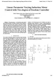
In order to limit the scope we will focus on a particular type of controller, more specifically the rotor-flux oriented controller as discussed in for instance [Rasmussen, 1995], [Vas, 1998], or [Leonhard, 1990]. This controller consists of subblocks as shown in Figure 1.1. ω r,ref i mR,ref

speed and magnetising current control

i sr,ref

stator current control

usr,ref

power device

us

induction motor

shaft load

estimates

observers

measurements

Figure 1.1: Sketch of the rotor flux oriented speed control scheme.

k | The controller objective is to track references for the magnetising current, , and p the speed, . The observers provide estimates of the stator and magnetising currents and of Q the speed. The speed and magnetising current controllers provide a reference p p signal, , for the stator current. The stator current controller tracks this reference Q p p by providing the power device with a stator voltage command, . The main aim of this thesis is to provide novel methods for designing these sub-blocks using LPV control theory. The theoretical parts will focus on the method described in [Scherer, 2001], which is very general and non-conservative.

1.3

Contributions

The contributions of this thesis are in both the induction motor application and the LPV control theory areas. The main contributions in the theoretical area are:

§ A discrete time version of the continuous time LPV control method presented in [Scherer, 2001] is given. § The current equations of the induction motor have a particular structure, which allows them to be written on a complex form. It is shown that for an LPV system with this structure, the optimal controller will also possess this structure. § A systematic approach for transforming neural network state space models into

4

Introduction quasi-LPV models suitable for control design is given. This was presented in the conference paper [Bendtsen and Trangbæk, 2000b].

§ A novel approach to robust LPV control for a special class of LPV systems is presented. This has partially been presented in the submitted journal paper [Bendtsen and Trangbæk, 2000a]. The main contributions in the induction motor application area are:

§ It is pointed out that the proof of convergence for the speed observer presented in [Kubota et al., 1993] is incorrect and that divergence is possible. § The discrete time version of the LPV theory is applied to the design of a flux observer. This has partially been documented in the conference paper [Trangbæk, 2000]. § The discrete time version of the LPV theory is applied to the design of a stator current controller using the quasi-LPV approach. This has been documented in the submitted journal paper [Bendtsen and Trangbæk, 2001b]. § A neural network is applied for black-box identification of the motor system. § The obtained neural network model is transformed into a quasi-LPV model and a speed controller is designed. § The robust LPV control method is applied to the same model.

1.4

Outline of the thesis

The thesis is organised as follows:

Nomenclature Provides a list of symbols and abbreviations used throughout the thesis.

Chapter 1 - Introduction This introduction.

1.4 Outline of the thesis

5

Chapter 2 - Preliminaries Introduces some basic concepts needed later in the thesis. The theoretical parts of Chapters 5-7 rely heavily on matrix inequalities and in particular linear matrix inequalities (LMIs). These concepts will be briefly discussed. The model structure used in the same chapters is linear fractional transformations (LFTs). This chapter also discusses interconnections of such systems including the Redheffer star product. Finally, the use of multi-layer perceptrons (MLPs) as state space models is discussed.

Chapter 3 - Induction Motor System Describes the dynamic model of a symmetrical three-phase induction motor with a squirrel cage rotor. The part of the model describing the currents is written as a complex second order state space model with the shaft speed as a time-varying parameter. The concept of rotating reference frames is then discussed. In order to control the speed of the motor it is necessary to use a power device. A commonly used type of power device, the voltage sourced inverter, is described. Finally, the laboratory setup is discussed. Experiments will be performed on a laboratory ¨ª©¬«U system with a induction motor.

Chapter 4 - Rotor Flux Oriented Control The rotor flux oriented control scheme for the induction motor is described. The purpose of the controller is to track a reference speed and a reference magnetising current while rejecting disturbances from the load torque. First it is discussed how the dynamical equations of the motor are simplified by writing them in a reference system following the angle of the rotor flux. Then the rotor flux oriented control method is described. The method is observer-based and requires an estimate of the rotor flux. A short discussion of flux and speed observers is also given.

Chapter 5 - Linear Parameter Varying Flux Observer This chapter reviews the LPV synthesis method in [Scherer, 2001] and applies it to the design of a flux observer for the induction motor.

6

Introduction

First the historical background of LPV control is reviewed. Then robust quadratic performance analysis of LPV systems is discussed and the so-called full block S-procedure controller synthesis is described. A discrete-time version of these results is then given. Considering the speed as a time-varying parameter allows writing the induction motor model as either a real fourth order LPV model or as a complex second order LPV model. This is due to a special symmetry in the transfer function. Theoretical justification for the fact that controllers and observers for this type of system can be assumed to have the same type of symmetry without loss of performance is presented. Finally a discrete-time flux observer is designed using the above theory. The observer is tested on the laboratory setup.

Chapter 6 - Quasi-LPV Current and Speed Controllers The quasi-LPV approach allows the use of LPV theory for a very general class of nonlinear systems. First a discussion of the quasi-LPV structure is given. The approach is then applied to the design of a stator current controller. It is then discussed how to transform a neural network state space model into a quasiLPV model suitable for control design. This method is then applied to the design of a speed controller.

Chapter 7 - Robust LPV Speed Controller In this chapter a novel approach is given for robust LPV design for systems where the time-varying parameters are uncertain. The method is applied to the design of a speed controller.

Chapter 8 - Conclusions This chapter contains conclusions and recommendations for further work.

Appendix A - Experimental Setup In this appendix the experimental setup is discussed in detail.

1.4 Outline of the thesis

7

Appendix B - Lemmas and Proofs This appendix contains lemmas with no appropriate place in the main thesis as well as proofs which were deemed too long and tedious for the main thesis.

Bibliography Index

8

Introduction

Chapter 2

P RELIMINARIES This chapter introduces some basic concepts needed later in the thesis. The theoretical parts of Chapters 5-7 rely heavily on matrix inequalities and in particular linear matrix inequalities (LMIs). These concepts are described in Sections 2.2 and 2.3. The model structure used in the same chapters is linear fractional transformations (LFTs). Section 2.4 discusses interconnections of such systems including the Redheffer star product. Chapter 6 describes the use of multi-layer perceptrons (MLPs) as a basis for obtaining quasi-LPV models. Multi-layer perceptrons are described in Section 2.5, whereas the discussion of the quasi-LPV structure will be left for Chapter 6.

2.1

Notation

Most of the notation in this thesis is standard with the following exceptions.

Definition 2.1 (Hermitian part, Let

SUT$VW

+®¯- )

be a square matrix. Then

SUT$VW

+,°-²±

¨ ³ P+ ´\¥ # -

10

Preliminaries

The Hermitian part is a natural extension of the real part of scalars, since the eigenvalues of a Hermitian matrix are real. The symbol µ is used as a right annihilator in e.g. [Scherer, 2001] and as a left annihilator in e.g. [Helmersson, 1995]. To avoid confusion when comparing with other literature we shall use the symbols ¶ and · respectively.

Definition 2.2 (Left annihilator, · )

>@ denotes any full row rank matrix such that

cTV

>@

F`W

.

>@ only exists if has linearly dependent rows and then @¸ Definition 2.3 (Right annihilator, ¶ )

>A denotes any full column rank matrix such that Note that

F¹W

># A

F`W

F`W

c¬TV

A

5 .

.

>@ # .

Finally, in order to reduce the width of certain matrix equations we will need the following notation. Given a matrix and a Hermitian matrix º the following expressions are » » » »¹¿ » » equivalent

¨ ¼ # º¼ ½¼

½¼ # º>¼ ¼g¾

2.2

Matrix inequalities

^ :O_G:

A square matrix is Hermitian if Ã . Let : denote the linear space of : U _ : ° # ^ Hermitian matrices and let ÀÂÁ . Let Ä½ÁÅ and define the quadratic form Æ Æ Ç ¨ Ä ± Ä # ÀYÄ È (2.1) We say that À

is positive semidefinite if Æ Æ Ç Ä C]5ÊÉxÄ

and that À is positive definite if ËGÌ

Æ Æ Ç 485ÎÍ Ä C

Ì

Æ Æ Ä

(2.2)

ÉxÄ

¨

(2.3)

We simply denote this ÀÏCÐ5 and ÀÑ4Ð5 , respectively. ÀÏDÐ5 (negative semidefinite) ËGÌ are defined similarly. Ì Ò is a positive subspace of À if and ÀÂ785 (negative definite) Æ Æ Ç Æ Æ 465"Í Ä C Ä ÉxÄÁÓÒ (2.4)

2.2 Matrix inequalities

11

and we write this as

¨

ÀÂ465 on Ò A negative subspace is defined similarly.

A Hermitian matrix has real eigenvalues and the maximal dimension of its positive subspace is equal to the number of positive eigenvalues. Consequently a Hermitian matrix is positive definite if and only if all of its eigenvalues are positive.

Definition 2.4 (Inertia,

Fà

)

The inertia of a Hermitian matrix Ô is defined as Fà Fà× 3 FàUØ 3 F¹aÃÙ +PÔb-Õ±Ö+ +ZÔ¦+ZÔ¦+PÔ¦-(2.5) Fà × 3 Fà Ø 3 Fà Ù +PÔ¦+ZÔ¦+PÔ¦- denote the number of negative, zero and positive eigenwhere values of Ô , respectively.

Fà ÆªÚ Definition 2.5 (Inertia on subspace, +® - ) : For any subspace ÒÛ8Å , ÆÜ Fà `F a +PÔ - ± l Z+ Ý # Ô¦Ýl-

(2.6)

for any basis matrix Ý of Ò . The following lemma is a generalisation of the well-known Schur complement lemma.

Lemma 2.6 (Schur complement) [Scherer, 2001] If is non-singular and and

FàÞ>ß £

are Hermitian then

£ #àuáUâ

Fà

+P>-\

Fà

+P

ã£

#

× K £

-

(2.7)

This lemma is very useful in many situations. An example will be given in Section 2.3.2. The following lemma will be used in the proof of Lemma 2.9.

Lemma 2.7 (Dualisation Lemma) [Scherer, 2001] Let FàGØ º Æ Ü be any non-singular Hermitian matrix, and let Ò be any subspace such that +Pº 5 . Then × K Æ ÆÜ Fà Fà Üæå

Fà (2.8) +ZºY+Zº -ä\ +Pº -

12

Preliminaries

^ :Ã_G: Now let ÀçÁ be a matrix function of a vector of decision variables . We will call Àè+ -485 a matrix inequality in . The feasibility set of a matrix inequality is defined as ' 3 é ± Í¬Àè+ -465 ) (2.9) and we say that the matrix inequality is feasible if é is non-empty. Of course 4 can be replaced by C , D , or 7 in the above. Remark 2.8 The decision variables are usually in the form of one or more matrices, but the problem can always be reformulated into the vector form. Matrix inequalities arise in many control analysis and synthesis problems. There is no general way to solve them, except when À depends affinely on . In this case, the affine matrix inequality can be solved with convex methods. This will be discussed further in Section 2.3. If the matrix is a quadratic function of there is generally no way to solve the inequality except in special cases such as the following.

Lemma 2.9 (Elimination Lemma for quadratic matrix inequalities) [Scherer, 1999] [Helmersson, 1999] £ Assume that has dimension and that Fà

3 3 +PºY+ 5 ä(2.10) The quadratic matrix inequality 9 # ß £ º >#;¦ê\ á in the unstructured unknown

ß

9 >#;¦ê\

£ á

785

has a solution if and only if 9 # 9 ß ß # A £ º £ A 765 á á

(2.11)

(2.12)

and

ß A #

=£ £ × K = ß # # # 9 9 º A 4]5 á á

(2.13)

Proof: A constructive proof is given in Appendix B on page 173. ë Remark 2.10 being unstructured means that there are no constraints on the structure, e.g. that it must be Hermitian or block diagonal. This lemma is the basis for the synthesis method described in Section 5.3.

2.3 Linear matrix inequalities

2.3

13

Linear matrix inequalities

As mentioned in the previous section there is no general way to solve matrix inequalities. However if the matrix depends affinely on the decision variables it is called a Linear Matrix Inequality (LMI) and fast and efficient numerical solvers are available. If a problem can be cast as an (finite-dimensional) LMI it can therefore be considered practically solved. This section contains a formal definition of an LMI, a short description of some of the available software packages and the types of problems they can solve, and finally a few examples of control problems that can be cast as LMIs. A more thorough discussion can be found in [Boyd et al., 1994].

Definition 2.11 (Linear matrix inequality, LMI) A linear matrix inequality is an inequality

Àè+ -(485 where À is an affine (i.e. a constant plus a:Ãlinear) function mapping a finite dimensional ^ _G: vector space to a Hermitian matrix set . The elements of the vector are called the decision variables.

Remark 2.12 In the usual definition the mapping is to a set of real symmetric matrices, and belongs to a real vector space. Indeed, most available solvers work only with this formulation. The above definition can however be reformulated as an equivalent problem with real matrices of double dimensions. This will be discussed further in Section 5.5. LMIs have several nice features. For instance the feasibility set is convex. This means that given a set of solutions of an LMI, any convex combination of these is also a solution.

Definition 2.13 (Convex combination) '.î K 3 î 3¨¹¨í¨¹3 î :

' K 3 3$¨í¨¹¨í3 : : Let ì space, and let ) be a subset of a linear vector ) NíðñK î N be a set on non-negative real numbers such that ï . Then : ò î N N ± N¹ðK is called a convex combination of ì

.

"! Definition 2.14 (Convex hull, ) "! The convex hull, +ZìÑ- of a set ì

is the intersection of all convex sets containing ì

.

"! +PìÑ- is the set of all convex combinaIf ì is a subset of a linear vector space, then tions of elements in ì . The convexity of the feasibility set can be used to convert some infinite-dimensional problems into finite-dimensional ones.

14

Preliminaries

Example 2.15 Consider the problem of finding an

such that

=ó\ã # # 485 (2.14) Q Q Q for all BÁ , where is convex. If has infinitely many elements, then this is an infinite-dimensional LMI, since (2.14) puts infinitely many constraints on . For a fixed we can also view (2.14) as an LMI in . This means that if fulfills (2.14) for a number of s, then it is also a solution for a convex combination of these. Q K 3 3¨¹¨¹3 : Now if is the convex hull of a finite number of vertices (or generators) Q, we only need to solve (2.14) for these vertices in order to obtain a solution for all Á . This is a finite-dimensional problem. LMIs rarely have an explicit solution but must be solved by numerical iteration. One exception is the LMI in given by

Àè+,°-

# ¦ê\ # # \¥¤Ï485

¨

(2.15)

This inequality typically needs to be solved as a last step in a controller synthesis, where , , and ¤ have been found as solutions to other LMIs. By multiplying from both sides by A or "A it is immediately obvious that

A # ¤ô A 4]5 and A # ¤ô A 465

(2.16)

are necessary conditions for the feasibility of (2.15). In fact they are also sufficient. This was shown in [Gahinet and Apkarian, 1994], where a constructive proof can also be found. Here we will give an alternative proof based on (2.15) being a special case of the quadratic matrix inequality (2.11).

Lemma 2.16 [Gahinet and Apkarian, 1994] ^ :Ã_G: Let ¤õÁ . The LMI (2.15) in is feasible if and only if (2.16) is satisfied. Proof: (2.15) is a special case of (2.11) with

£ \

£ #

¤ ,º

ß 5 9 :

9 : 5çá

¨

The inertia condition (2.10) is then immediately fulfilled and the conditions (2.12) and (2.13) can easily be seen to be exactly (2.16). ë

Remark 2.17 Since the proof of Lemma 2.9 is constructive, this proof can also be considered constructive.

2.3 Linear matrix inequalities

15

Remark 2.18 In Lemmas 2.9 and 2.16 7 can of course be replaced by 4 and vice versa, but the sufficiency parts do not hold for non-strict inequalities ( C and D ). Consider for instance the non-strict LMI

ß ¢ Õ\ ¢ Àè+ ¢ C]5 $#Õ\ ¢ l\ $#Õ\ ¢ á in the real scalar ¢ . This can be written as (2.15) with »

´\¥ #

¢ 3

ö ¼

3 ¤

ß 5 ¨ $#÷Õ\¥é# á

K ³ ³ À + ¢ - has eigenvalues + ¢ \q\6$#(ø ù + ¢ \ l\ # - \¥ú¬; # - which are clearly of è ¢ different signs no matter how is chosen. In other words the non-strict LMI Àè+ ¢ -CÈ5 has no finite solution, but the non-strict versions of the conditions (2.16) both read » » ßþ

3 û A # ß 5 ý A ßþ # ß 5 5ÎC85 ¼ ¼ þ á þ á # ü\ # á # l\ # á where þ is an arbitrary non-zero number.

2.3.1 LMI solvers Several software packages are available for solving LMIs. The most widely used is probably the LMI toolbox for MatLab [Gahinet et al., 1995]. Free alternatives are LMITOOL [Nikoukhah et al., 1995] and sdpsol [Wu and Boyd, 1996]. The MatLab toolbox can solve three different types of problems in addition to an explicit solution of (2.15). The first is the feasibility problem:

§ find, if it exists, a solution to the LMI Àè+ -4]5 . The second problem is the linear objective minimisation problem:

§ WèFà ' Í¬Àè+ -485 ) . This is a generalisation of the eigenvalue problem: 5 ) .

WèFàUÿ ' 9 3 Í Àè+ -485 + -4

The third problem that can be solved by the MatLab toolbox is the generalised eigenvalue problem:

§ WèFàæÿ ' Í

3 3 + Àè+ -465 + -485 Ô¥+ -465 ) .

16

Preliminaries

The first two problems are convex and are solved by interior point methods. The third is only quasi-convex but can be solved by similar techniques [Gahinet et al., 1995]. It is beyond the scope of this thesis to discuss how these methods work. For an introduction to interior point algorithms in convex programming see [Nesterov and Nemirovski, 1994] or [Nemirovski and Gahinet, 1994] describing the algorithm used in the toolbox.

2.3.2 Examples of LMIs in control Two examples of LMIs arising in connection with control problems will be given here. For more examples see [Boyd et al., 1994] and [Packard et al., 1991].

Lyapunov stability Consider the autonomous system

3

where is a constant square matrix. This system is Lyapunov stable if and only if there exists a positive definite Lyapunov matrix such that ¨ # ó\ãbÈ765 A test for stability can therefore be cast as a feasibility problem in X: ß >#; ¨ ¦ 5 4]5 5 á

Riccati inequality control problems often lead to Riccati inequalities such as £ £ 3 # 785 # ´\ãb \¥]+P[ # ¤ô¤ # -ó\

485

¨

Because of the quadratic term this is not an LMI in . However, if we assume [²#"4 ¤ô¤ # (meaning [ # ¤ô¤ # 465 ) then we can use Schur complement (Lemma 2.6) to arrive at the equivalent £ £ ß >#ó\ãb \ 3 # × K (2.17) 785 485 +Z[²# ¤ô¤Ó#$- á which is indeed an LMI in . If on the other hand "Î# ¤ô¤# is indefinite then we £ £ × K cannot use this trick. But if # is non-singular (and consequently positive definite)

then we multiply from both sides by to arrive at £ £ 3 ¨ # 765 " # \ \+Z[ # ¤¡¤ # - \ 465

2.4 Linear system interconnection

17

This can then be converted into an LMI in . A problem with this last approach arises × K are LMIs. if (2.17) is just one of several constraints on even if the other constraints

Then we will have LMI constraints on and but also the constraint which is not convex. This problem arises in most robust synthesis problems.

2.4

Linear system interconnection

This section is a short introduction to the interconnection of linear systems. The concepts of linear fractional transformations and Redheffer star product will be described. For further details see [Doyle et al., 1991], [Zhou et al., 1996], and [Helmersson, 1995]. KK K

ß K Let be a complex matrix. Then the lower linear fractional transfor á R e mation (LFT) with respect to is defined as [Doyle et al., 1991] × K KK K R e 9 K ¨ R e d(e 3R e

+ -l ± \ + - R The upper linear fractional transformation with respect to is defined similarly as K K R f 9 KK R f × K ¨ dgf 3R f + -l ± \ + - The transformations are only defined if the inverses exist.

Definition 2.19 (well-posed, well defined) d(e 9 3R e The lower LFT + - is said well-posed (or well defined) if dgf to be 9 3R f

+ - is said to be well-posed if non-singular. The upper LFT non-singular.

R e KK R f is is

The LFTs are another formulation of the interconnections in Figure 2.1. Often deR scribes a known and time-invariant system and contains unknown or time-varying gains.

M ∆l

∆u

M

Figure 2.1: Lower and upper linear transformations.

18

Preliminaries

The Redheffer star product, h , represents the interconnection in Figure 2.2, i.e. K K ß ß

h +Z " á á Note that h depends on a partitioning of and . This partitioning will always be clear from the context. K K

¾

K

K

h

Figure 2.2: Redheffer star product. Let the partitioning be given by

KK

ß

K

K

and á

have [Doyle et al., 1991]

h

d(e 3 KK K 9 P+ K K - × K K + - ß

KK

ß

K

. Then we á K

× K K K K +9 - ¨ dgf 3 á +Z K

Again we need the inverses to be defined.

Definition 2.20 (well-posed,well defined) We say that the interconnection h non-singular.

is well-posed if

9

Remark 2.21 The star productd is defined even if for instance f

3 . Then h +P - . i.e.

KK K

KK 9 are and and

K

are of zero size,

The star product is associative [Helmersson, 1995] i.e.

£

£ ¨ +Z h "- h h +P h ß5 Furthermore 9

9 5 á

is the unit element of the star product or star product identity, i.e.

ß5 h 9

9 5 á

ß5 9

9 5 á

h ¨

2.4 Linear system interconnection

19

These two facts can be used for transforming problems into special forms. The following example demonstrates how to do this if a given design method requires a system to be strictly proper. The example system has more inputs and outputs than needed to demonstrate the idea, but it has been chosen this way, so that it can be directly applied to the theory described in Section 5.3.

Example 2.22 The synthesis method described in Section 5.3 requires the system f f f ff f gf £ f

þ

¤ ¤ (2.18) f £ þ ¤ ¤ f £ ¢ À À À to be strictly proper in the channel from the control signals, , to the measurements, ¢ , i.e. À must be 5 . Then (under some assumptions) a suboptimal controller on the form K Ã Ã £ K ¤ KK ¤ K ¢ (2.19) K £

þ ¤ ¤ can be constructed. The meaning of the signals for now, and will be discussed in Chapter 5.

f 3

3

3 þ f 3 þ , and þ is unimportant

In practice it may happen that the system we wish to design a controller for is not strictly proper. This problem can be overcome by finding a controller for the corresponding

system with À 5 and then transforming the controller into another controller yielding the same closed loop system for the actual system. Denote the system matrix in (2.18) by and define 9 9 ×

ß5 3

ß5 9 9 À á À á and observe that

× h

×

and that

±

h

ß5

h

9

£ f £ £

9 5.á f f f ¤ ;f ¤ f À

is the Redheffer star product identity,

f ¤ ¤ À

f

¨

5

Now assume that a controller, , has been obtained for the system defined by write this controller as K K ¢ £ K ¤ K ¤

3

¨ K £

þ ¤ ¤

, and

20

Preliminaries

Then, assuming that

9

\¥À

is non-singular, the closed loop is given by

þ

þ

f

þ

f

in which

±

h h +

×

h + h h - +

×

h

-

- h

h +

A controller for the system defined by is thus given by ¢

3

¨ + h þ

2.5

h

-¨

(2.20)

Multi-layer perceptron

This section provides a short introduction to a particular type of artificial neural network, the multi-layer perceptron (MLP), which can be used to model nonlinear functions. It is beyond the scope of this thesis to go into detail with this subject. For a more thorough introduction see for instance [Suykens et al., 1996] or [Bendtsen, 1999] and the references therein. First the MLP structure will be discussed. It is then discussed specifically how to obtain nonlinear state space models from input and output measurements using the MLP structure. The multi-layer perceptron (MLP) is composed of layers of perceptrons coupled in parallel. A perceptron consists of a memoryless scalar function, the neuron function, acting on a weighted sum of input signals, as shown in Figure 2.3. The neuron function (or simply neuron) can be either linear or nonlinear. Some of the traditional neuron functions in MLPs are the unit gain eN:

+ and the hyperbolic tangent !

: #" HaUS

+ + -

× ° ¨ × \

2.5 Multi-layer perceptron K K .. .. . : . : *)

21

%& $ '

+-,/.10 (

(

+ï

:

N¹ðK N N ) \ -

Figure 2.3: A single perceptron. In this thesis only these two will be used. A blockN : diagram of an MLP with one hidden layer K is shown in Figure 2.4. The input ) vector þ is multiplied by the input weight matrix 2 . The bias vector 2 is then added and the sum is input to containing a number of neurons in parallel. The resulting output f is multiplied by weight matrix 2 producing the final K 3¨¹the K output 4þ 3 . Notice*that ) : ¨í¨¹3 output the weights in Figure 2.3 form a row in the matrix 2 and that the weight is ) an element in 2 . The output weight matrix 2 can be seen as stemming from a layer with linear neurons and no biases. The resulting function is K N: N: 3 K 3 ) f

k 3 ) ¨ þ 3 4 þ # (2.21) 2 5+ 2 \ 2 -Õ6 ± +þ 2 2 2 K ) By choosing 2 , 2 , and 2 appropriately the MLP can be used to approximate a given static nonlinear function. It has been shown [Hornik et al., 1989] that with a sufficient number of neurons and under certain continuity conditions, the MLP with one hidden layer can act as a universal approximator.

N: þ 2

( 2

K (

( 7

+®ª-

( 2

(

þ43

f

)

Figure 2.4: Block diagram of an MLP with one hidden layer.

2.5.1 Training Adjusting the weights of a neural network is known as training. For an MLP this is typically done by trying to approximate a set of output targets in the following manner. K 3¨¹¨í¨ þ k and a corresponding set of input vectors þ Given a set of target output vectors N : K 3¨¹¨í¨¹3 N : k þ þ Ì define the approximation error N: k 3 K 3 k f k

k k 3 ) þ 3 4 þ + -Õ± þ +þ 2 2 2 -

22

Preliminaries

and the quadratic performance functional

i

ò

Ì

«9N¹ð8 K ³

Ì + -
p

C¬ C C

)

3

+Z+P-

3

>p 3 +P-

, is the resistance of the (virtual) rotor windings.

3.1.3 Complex space vector notation To simplify the equations a complex notation based on the value ± duced. The complex space vector of the stator current is defined as ³ Q ¨ +Z-Õ± Z + N O +P-\ N P +Z-ä\ 1 Q +Z-For the rotor currents a space vector is defined as well: ³ Q p p p p) ¨ +P- ± Z + +Z-ä\ +P-\ P+ --

¬

is intro-

(3.17)

(3.18)

34

Induction Motor System

Notice that no information is lost in this transformation from three to two degrees of freedom. Using (3.1) the three stator currents can be reconstructed from the space vector. p p) p

Similarly the rotor currents can be reconstructed due to \ \ 5 . The space vector for the stator voltage is ³ xQ +P-Õ± Zl+ ] O +Z-ä\ ñxNP +P-ä\ 1Q +Z-- ¨

(3.19)

The three stator voltages cannot be reconstructed from this value without adding an

, where is some chosen additional demand, for instance NO +P-x\ NP +P-x\ 1Q +Pconstant, but due to the isolated neutral the value of this constant is of no importance. We also define space vectors for the stator and rotor flux linkages: ³ Q 3 +Z-Õ± Z + N O +P-\ N P +P-ä\ 1 Q +P--

Q p

+Z-l±

³ Z

p +

p p) ¨ +P-ä\ P+ -ä\ +P--

(3.20)

(3.21)

Inserting equations (3.8), (3.10), and (3.11) in (3.20) after some calculations gives: qp Q j k Q p

j Q m {on 3 +P+Z-ä\ +Z(3.22) j j k where the stator inductance, , and the mutual inductance, are r r r[p j Z X Z X hP 3 j k hP ¨ ± ` 3 r ± ` 3 b (3.23) r Ä Ä A similar equation can be obtained for the rotor: × qp Q p > j k Q m { n 3

jlp Q p +P+P-ä\ Z+ j p where the rotor inductance, , is r p j p Z X h, ¨ ± ` 3 r Ä

(3.24)

(3.25)

Combining (3.14)-(3.16) with the space vector definitions (3.19)-(3.17) results in the simple equation: Q +Z- ¨ Q +P- s Q +Z-ä\ C (3.26) C A similar result can be obtained for the rotor:

5

s p Q p

+P-ä\

C

Q p > C¬

+P- ¨

(3.27)

3.2 Stator-fixed coordinates

35

By inserting space vector expressions in the flux density equation (3.4) and inserting this in the torque equation (3.7) the integral can be calculated to get the following expression for the electro-magnetic torque tangential to the rotation: Z qp +P- ³ j k &(' Q +Z-;+ Q p +P- m { n - # ) ¨ (3.28) Inserting (3.22) and (3.24) in (3.26) and (3.27) gives: qp Q +P- s Q +Z-ä\ j C Q +Z-ä\ j k C + Q p +Z- m { n C¬ C × qp j p C Q p j k C Q m {on ¨

s>p Q p 5 +Z-ä\ +P-ä\ + +PC C¬

(3.29)

(3.30)

3.1.4 Mechanical system k The mechanical rotational speed is affected by the electro-magnetic torque and the load torque y : k +P- i"+ +P- y +Z-- 3 (3.31) i where is the collective moment of inertia of the rotor and the load, assuming the shaft to be rigid. y contains the actual load along with the speed-dependent viscous and coulomb friction. The electrical rotational speed is defined as p +P- p Z+ -

k ¨ +Z-

(3.32)

Equations (3.28)-(3.32) form the model to be used below.

3.2

Stator-fixed coordinates

The model of the induction motor can be expressed in various coordinate systems. Expressing the model in a coordinate system which rotates with the rotor or statorp flux gives a model in which the states are constant in steady state operation (constant and y ). This model is often desirable for control purposes but in order to perform the non-linear change of coordinates it is necessary to know the rotor flux angle. For flux estimation purposes it is therefore often desirable to work with a model in stator-fixed coordinates. Q Q p Q In (3.29) and (3.30) and are already in stator-fixed coordinates, while is in rotor-fixed coordinates. By defining the stator-fixed rotor current qp Q p Q p m o{ n +P- ± +Z(3.33)

36


the following stator-fixed model is found:

+ jlk +

C C

s j \

C C¬

Q jlk - P+ -ä\

C C¬

Q s p j p ½ p +P-- P+ -ä\ê+ \ + +P-

p Z+ -

Z

³

Q p

Q 3 +P+ZC C¬

(3.34)

Q p ½ p

3 +Z--- Z+ 5

ñvj k &(' Q Q p 3 Z+ Z+ - # )

k

+Z-

(3.35)

(3.36)

¨ y +Z-i + +P-

(3.37)

Q Q p Q To summarise, and are the stator and rotor currents. is the stator voltage, which p is often controlled through a voltage sourced inverter as described in Section 3.5. is the rotational speed of the rotor. p is the electro-magnetic torque. y is the load torque s s j j p j k , , , , , and are the parameters of the motor, acting as a disturbance. i and is the collective lumped moment of inertia of rotor and load.

3.3

State space model

For several analysis and synthesis methods a state space model is desired. This model will be formulated here. For convenience the time dependency will be dropped in the notation. From (3.34) and (3.35) a complex state space model for the current equations can be obtained: p p p \ p Q 3 Q 3 æ ß Q p á

Ù = y × y ~xu w { × y { uy ~ × y yu w { yG{y y ×{ p t

s yG{ y× u y ×~ y {y u

y { |vu p ts × y =~ | u y =~ y ~

~ n × | = { ×y ~ Ù yU{ w { y ~ × y {y u y u | {= × y u yG{ w { y ~ yG{y u = y ~ ¨ y =~ y p

3 y

p The speed could be included in the state vector as a third state, but the above form has the advantage that the state space part can be seen as a linear parameter varying system p with as the varying parameter, see Chapter 5.

3.3 State space model

37

3.3.1 State transformations

Q ß For control purposes it is often desirable to work with another state vector than Q p . A á state transformation is obtained by multiplication of a state transformation matrix, T, × K : :

w pw 3

w p : Nz w 3 (3.38) Nz ]z An important choice of states is

± Q k

The magnetising current, Q p

Q ß Q k á

s

5 yG{ y ~ y

Q ß Q p á

¨

(3.39)

, has the same angle as the rotor flux Q p m { jlk Q k j k Q j p Q p ¨ ± \

The resulting state space system is

Q \ 3 ß Q k á= = = Ù y ~ |={ × | u y { p y ~ n

s yU{ n y ~ y u yU{ yU{ n y | { y { y ×{

s y u y { y =~ t 5 = {W | y y { ~ &(' Q + Q k Q - # )

p

k {W} | +

(3.40)

Q 3 × p yU= { × w { | { p ~ y |u U y { p { y { 3 y

3 y

(3.41)

=

{W| y ~ ( & ' Q Q k 3 # ) y { ¨ y -

This particular choice of states has some nice properties for control purposes which will be discussed in Chapter 4.

3.3.2 Real state space model To obtain a real state space model the space vectors are first split into real and imaginary parts: Q ]~ \ 1 3 (3.42)

Q ]~ ¬ 1 3 \

(3.43)

38


Q k

6 k

k

~

¬ k \

3

(3.44)

k

where xN~ , 1 , N ~ , 1 , ~ and are real signals. A real state space model can now be obtained by substituting the complex system and input matrices by real matrices of double size p N N ß p < N p (3.45) \ á and by substituting the signal vectors

p ß ¨ Ná

p \ N This gives the following model:

p

p

=

y ~ | y U{ n y

p

{ ~| =

= Ù v × | uu y { y y { { yG{ 5 5

p p p p \ N~ k ~ N k

× = | y ~× { y {[n y =~ | y u y { { = yG{ ~ w { = y × y ~ y u yG{ p y { y u yG{ × y =~ p

5 5 5

Z ñvj

³ jlp

k

ß ]~ x1

3 p

p

(3.46)

p =

5Ù

=

y ~ |={ × | u y {p yG{ n y ~ | y u yG{ { y { 5 3 5 yG×{ = y uy { y ~ 5 ~

° N~ k

=

~ w y × y p × = | =y ~ × y { ny ~ | y G { y {

5

k + 1

p

k

á

-

¨ y i +

3

y =~

{ u

{ u

y { yG{

p

3

(3.47)

(3.48)

3.3 State space model

39

3.3.3 Rotating reference frames In normal operation the inputs and states will be rotating, i.e. following circular trajectories in the complex plane. For control and simulation purposes it is often desirable to work with the system in a rotating coordinate system. Defining the signals × × p ± p ± (3.49)

\¥ can be the system written as p +P ½ 9 - p \ p (3.50) where ± .

3.3.4 Steady state In normal operation the space vectors will rotate around the origin in the complex plane.

Definition 3.1 (Steady state) The complex state space system

\

(3.51)

is in steady state if there exists a reference frame rotating at angular velocity such that p +P ½ 9 - p \ p 5 , and p 5 3 (3.52) p p where and are defined as in (3.49).

k

% Q Let the system (3.41) be in steady state and define | such that k ½ | ¨ Q

+P \ 5 (3.53) Q Q × ~ ~ ß ß × w @ 3 Q Q w @ Q k ± Q k Then ± are all constant and the states are á á given from Q × K ß k | Q Q k +Z - á as

Q

s>p k p j p x Q \ + | - - s s p k k k p s j p k j s p p j k j p j \ + | \ | \ | + | -;+ +

(3.54)

40


Q k

s p Q ¨ s s p k | k | p j k j p j k | p s j p k | j s p \ + \ \ + -;+ (3.55)

eN The quantity ± by

k | p is known as the slip frequency and is related to the torque

3.4

Z

j k Æ Q k Æ eN ¨ ³ s p

(3.56)

Uncertain and time-varying parameters

The dynamical behaviour of the induction motor is affected by time variations in the parameters. s p The rotor resistance can change as much as 50 % due to heating. Furthermore it can be difficult to obtain an accurate estimate of its value especially during steady state operation. s The stator resistance can also change, but the stator windings are usually better ventilated than the rotor windings, so the variations will not be quite as large. In addition obtaining an accurate estimate Since both of these variations are caused by s p is easier. s and will be slowly varying. temperature changes, both p The rotational speed can change due to load disturbances or as a result of a command change to the controller. This variation will typically be fast p compared to some of the p other dynamics of the motor. Sometimes (or the position ) is measured, but avoiding the use of a speed (and position) sensor is often desirable, due to the relatively high cost and high sensitivity to the environment of these sensors. jlk j j p The mutual inductance (and to some extent and ) will be affected by magnetic saturation effects when the magnetisation changes. Notice that in the derivation of (3.29) and (3.30) it was assumed that these inductances are constant, so modelling this uncertainty is more complicated than simply assuming the inductances to be time-varying in the above model.

3.5 Power device

3.5

41

Power device

In a control context the control objective is usually controlling the angular velocity or position of the rotor shaft. The control signals are usually the stator voltages or currents depending on the type of power device. The description here will be limited to a (threephase bridge) voltage sourced inverter (VSI). For a thorough discussion of power devices including current sourced inverters see [Ka´zmierkowski and Tunia, 1994]. Figure 3.5 is a sketch of the power device in connection with the induction motor. The DC voltage source converts a three-phase AC supply to a DC voltage which is then supplied to the inverter. The signal conditioning supplies the inverter with a modulation signal to generate the reference stator voltages.

u s,ref

Signal conditioning U+,U-

PWM U+

AC supply

usB usC

UDC voltage supply

u sA

VSI

Induction motor

Figure 3.5: Voltage sourced inverter connected to an induction motor.

The inverter is sketched in Figure 3.6. By applying pulse width modulation signals k k k to the input terminals xNO z , xNP Ù z , and× NQ z the output voltages NO , ]P , x 1Q and can be switched between and . Since the stator currents only depend on the lower frequency part of the stator voltage this is equivalent to applying a low pass filtered version of the switched computes the voltages. The signal conditioning Q p modulation signals to accomplish + N O \ xN P \ x1Q -k x , where the approximation is only considered for the low frequency part.

42


u sB

u sA

u sC

U+

U–

u sA,pwm

u sB,pwm

u sC,pwm

Figure 3.6: Three-phase bridge voltage sourced inverter.

3.6

Parameter identification

s s p j k j For control purposes it is necessary to know the motor parameters , , , , j p and . These can be identified from stator current and voltage measurements. There is however an infinite number of motor parameters all yielding the same behaviour [Gorter, 1997]. It is therefore necessary to make some assumption on the paramj p j . The parameters can then be identified for ineters, for instance that stance by auto-commissioning at standstill as described in e.g. [Rasmussen, 1995] and [Rasmussen et al., 1995]. The voltage reference is chosen in such a way that the generated torque is not large enough to pull the shaft out of standstill. If voltage measurements are not available the reference voltages for the power device must be used.

3.7

Experimental setup

In this thesis several experiments will be performed on a laboratory induction motor system illustrated in Figure 3.7.

3.7 Experimental setup

43

power device

induction motor transducers

brushless DC motor

shaft

encoder

u s, i s

power device

θr mL,ref PC

Figure 3.7: Laboratory induction motor system.

ó³ The induction motor has two pole pairs ( ), a squirrel-cage rotor, and three star connected stator windings. Its nominal data are Nominal power 1.5 kW Nominal speed 1420 rpm Nominal torque 10 Nm Nominal current at 380 V 3.6 A ³

rU¨ î t The nominal speedî of ú 5. ú C _ is equivalentî tot the electrical rotational p t ê

³ G \ ¨ speed ú C _ . The electrical rotational speed in C _ will be the representation used in the following chapters. In [Rasmussen, 1995] the parameters j jlofp the induction motor were identified at standstill ³ £ at 5\ under the assumption as

j

j p

5

¨ Z ©³ Ô

3

jlk

5

¨Z

3 ú Ô

s È©¸¨ 3 5W

s p

Z ¨Z

¨

(3.57)

The PC runs the control program to be tested providing a reference voltage for the induction motor power device and a torque reference to the DC motor power device. The brush-less DC motor can be used to simulate a load torque on the shaft. Since the PC receives measurements of the rotor angular position from the encoder this can for instance be a position or speed dependent load. In addition to the encoder data the PC receives measurements of the stator current and voltage. The equipment is described in further detail in Appendix A.

44

3.8


Summary

This chapter described the induction motor system. The following complex state space model of the induction motor in the stator-fixed reference frame was derived: \¥ Q 3 Q 3 Ã ß Q k á = = Ù | u = × p y ~ |={ × v y { p y ~n y = { × w { | { p u u 3

t s y y y y y y y y { U n ~ { { U n ~ { | { p | { y yG{ yG{ y ×{ = u 3

s y yG{ y ~ y 5 = { | y ~ &(' Q Q k# ) 3 y { p ñ k { } | + y - ¨

Q Q k Q and are the stator current and voltage, respectively, and is the magnetising p current. is the rotational speed of the shaft. is the torque produced by the induction y is the load torque on the shaft acting as a disturbance. j k , j , jlp , s>p , s , motor. ñ i , and are constant or slowly varying real parameters. Q The stator voltage, , is the controlQ signal and is supplied to the motor by p a power Q device, the voltage sourced inverter. and , and in some configurations , can be measured. This constitutes the model to be used in the following chapters. Experiments will be performed on a laboratory system described at the end of this chapter and in Appendix A.

Chapter 4

ROTOR F LUX O RIENTED C ONTROL In this chapter the rotor flux oriented controller (or rotor field oriented controller) scheme for the induction motor is described. The purpose of the p controller is to track a reference p p k speed, , and a reference magnetising current, | , while rejecting disturbances from the load torque. The main purpose of this chapter is to present an existing induction motor control method. This controller is a cascade coupling of several sub-blocks. The aim of the following chapters is to develop replacements by new methods for some of these sub-blocks. It has therefore been chosen to focus on field oriented control and in particular the rotor flux orientation rather than give a full review of all the many control methods for induction motors. Section 4.1 shows the simplification in the dynamical equations of the motor achieved by writing them in a reference system following the angle of the rotor flux. Section 4.2 then describes the rotor flux oriented control method. The method is observer-based and requires an estimate of the rotor flux. A short discussion of flux estimation is given in Section 4.3. If a speed or position measurement is not available it is furthermore

46

Rotor Flux Oriented Control

necessary to estimate the speed. A brief introduction to speed observers is given in Section 4.4. The controllers and observers described in this chapter have all been described before. The only new contribution is the discovery of the potential instability of the speed observer described in [Kubota et al., 1993]. An example of this instability is given in Section 4.4.2.

4.1

Model in rotor flux coordinates

By expressing the model in a coordinate system fixed to the rotor flux angle % Q p % Q k 3 (4.1) ± Q k Q k Q y { Q p is as given in Section 3.3.1, i.e. \ y ~ , a partial linearisation of the where torque and magnetising current equations can be achieved. Equations (3.34) and (3.35) in rotor flux coordinates are:

+

s \ê+

C C

\

k | j m Q p - \ê+

s pm k | Q p + - \ê+

C C

\

C C

k | j mk k | x Q p 3 \

k | p j mk k |

3 + -5

where the following definitions have been used Q p Q × Q p , ± Q k × > k | k |

Æ k Æ , ± j m n ( j k t j p j ± + -, j mk s>pm ( on j j k tvj p , ± + -

±

± ±

±

(4.2)

(4.3)

× Q , , n j , jlktvj p s p . + -

The stator current in rotor flux coordinates is split into two real values, the direct and quadrature components: × * ' Q * ' Q p 3 ± ) × ) &(' Q &(' Q p ¨ ± ) )

k By taking the real part of (4.3), a dynamic equation for the magnetising current, | , can be found as j p C k | k | ¨ s p \ (4.4) C¬ w p y { The quantity ± | { is called the rotor time constant.

4.2 Rotor flux oriented control

47

The imaginary part gives the slip frequency

e N

¨ w p k |

(4.5)

The produced torque can be found from (3.28) as

Z

³

.j mk k | ¨

(4.6)

k As seen a decoupling is achieved so that isk used for controlling | and is used for controlling the torque . Even though | does affect , the changes are slow, making an almost linear function of .

4.2

Rotor flux oriented control

Several speed or torque control schemes for induction motors exist, see for instance [Ka´zmierkowski and Tunia, 1994] or [Vas, 1998]. Also worth mentioning is the passivity-based approach described in e.g. [Ortega et al., 1996]. In this thesis we will however focus on one particular type of induction motor control, namely direct rotor flux oriented control which will be described in this section. The basic principle is shown in Figure 4.1 and is based on the partial decoupling of the torque and the magnetising current achieved in the rotor flux oriented reference frame. ω r,ref i mR,ref

speed and magnetising current control

i sr,ref

stator current control

usr,ref

power device

us

induction motor

shaft load

estimates

observers

measurements

Figure 4.1: Sketch of the rotor flux oriented speed control scheme.

k The controller objective is to track references for the magnetising current, | , and the p speed, (or torque The observers provide estimates of the stator and magQ or position). Q k netising currents, and , and of the speed. These estimates are based on measurement Q of some of these three signals. In some cases the stator voltage, , is also measured. Q p p Otherwise the voltage command, can be used. The speed and magnetising current controllers operate in the rotor flux oriented reference frame and provide a reference

48


Q p p signal, , for the stator current. The stator current controllerp tracks this reference Q by providing the power device with a stator voltage command, , in the stator-fixed reference frame. Examples of how to implement the different blocks will be given in the following. The examples in Sections 4.2.1-4.2.3 are from [Rasmussen, 1995].

4.2.1 Speed control The speed can be controlled through the torque, , given by equation (4.6). Since the torque usually is not measured, nothing will be gained by estimating and controlling it in a feedback loop [Rasmussen, 1995]. Instead, the reference value for can be found from (4.6) as ³ p

p ¨ (4.7) Z j mk k | The speed can then be controlled for instance by a PI-controller tuned by a relay feedback experiment. Since the speed controller is in a cascade coupling with the stator current controller, the tuning must be performed with the intended stator current controller in operation. The tuning will also be affected by the bandwidth of the speed sensor or estimation. The torque is limited by the maximum stator current allowed. The limit is found as Z ñvj km k | 9 k ; b p ¨ k

(4.8) ³ Anti-windup must therefore be implemented if the speed controller contains an integration. The scheme is illustrated in Figure 4.2. The PI-controller acts on the control error p p p . The PI-controller output p is limited by k computed from (4.8). p p The torque reference is converted into a current reference using (4.7). ω

r,ref

me,ref

+ PI ^ ω

r

torque control

isq,ref

me,max maximal torque computation

î mR

Figure 4.2: Example of a simple speed control scheme.

4.2 Rotor flux oriented control

49

4.2.2 Magnetising current control k The magnetising current | is governed by (4.4). The aim of the controller is to keep k | constant at some predetermined value. At speeds above rated speed it may be necessary to reduce this value in order to avoid saturation of the voltage supply. This situation will not be considered here. Since the steady state transfer function is 1 independent of physical parameters a propor² K tional controller withÙ gain will have zero steady state error if the reference value is | premultiplied by | assuming that the stator current controller has zero steady state error. A proportional controller tuned by a relay-feedback experiment can therefore be used.

4.2.3 Stator current control As described in Section 4.2 a decoupling is achieved in the rotor flux oriented coordinate system so that controls the magnetising current and controls the torque. The stator currents and are controlled through the direct and quadrature components of the stator voltage, and , defined as * Q p 3 ± + & Q p ¨ ± + Unfortunately the equations for the currents are cross-coupled so a decoupling is necessary. Splitting (4.2) into the real and imaginary parts gives

x

x

+ +

s j m \

s j m \

C C¬ C C¬

j mk k | j m - \

C C¬

k | 3

j mk k | k | ¨ k j m - \ | \

(4.9)

(4.10)

Inserting (4.4) in (4.9) a decoupling scheme can be identified from

+

s j m \ +

C C¬

s j m \

k j m s pm ° k | 3 - \ | + -

(4.11)

k | j m j km k | k | ¨ -

(4.12)

C C

Decoupling can be achieved by adding the feed-forward voltages Ié ± k | j m \ s pm + ° k | - 3

(4.13)

50


± k | j m \ j km k | k |

(4.14)

to the outputs of the current controllers M and . We then achieve

s j m \ + +

s j m \

C C C C¬

- -

xM 3

x ¨

The stator current can therefore be controlled by for instance PI-controllers tuned by relay-feedback experiments. This k current k control system is illustrated in Figure 4.3. In practice the values of , , | , and | all have to be replaced by their respective estimates. Anti-windup again has to be implemented due to limits in the voltage supply.

î sd isd,ref -

isq,ref î sq

usdff PI

PI

usdc

usd

usqc

usq usqff

Figure 4.3: Example of a simple stator current controller.

4.3

Rotor flux estimation

In the stator current, magnetising current, and torque controllers estimatesQ of the magni p jlk Q k ) tude and angle of the magnetising current (or equivalently the rotor Q k flux are needed. This section will give an example of how to estimate based on measureQ Q p ments of , , and possibly . A flux observer can be based on respectively the voltage model (3.34) and the current model (3.35) or a combination of these. The observer based on the current model (3.35) is: s>p sp Q k Q p Q k + j p \ \ j p (4.15)

p s p Note that this model requires accurate estimates of and . It is essentially an open loop simulation of the motor regarding the stator current as input.

4.3 Rotor flux estimation

51

Another observer is based on integrating the voltage model Q Q s Q \ C C Q Q k to obtain an estimate for and then finding from j p jlpj Q k

Q ¨ Q g j k \ê+ j k -

(4.16)

(4.17)

p s p and , but it can be very noise The voltage model method does not need values of sensitive especially for low frequencies due to the pure integration.

4.3.1 Closed-loop observer of Jansen and Lorenz The rotor flux observer described in [Jansen and Lorenz, 1992], here called the JLobserver, is an example of a combination of the current and the voltage model. This observer combines the good qualities of the current model in low speed operation with the good qualities of the voltage model in high speed operation. The JL-observer is shown in Figure 4.4. is current model is

Rr Lm Lr

us -^ Ψrc

-

K1

Rr - j ω r Lr

g

K2

Rs

σ Lm 1−σ -^ Ψs

Lr Lm

-

1 -^ L m Ψr

^ im

voltage model

Figure 4.4: Flux observer of Jansen and Lorenz (JL-observer). K × K The - and -blocks constitute a frequency dependent weighting between the two K observer types. For frequencies, _ , where \ K_ is× K large (low frequencies), the 5 the JL-observer is main emphasis will be on the current model. For \_ exactly the voltage model observer. The idea is that at high frequencies we can exploit p s p the robustness of the voltage model to uncertainties in and and at low frequencies we can use the current model which has lower gains and therefore is less noise sensitive.

52


The JL-observer can be written as the state space system:

e e Q k £ e

e e k 3 \ ¢ e e¢ k 3 \¥¤ Q e L 3 Q p Q 3 ¢ k ß Q á

e

e

£ e y = { y ~

4.4

; yG{ K y ~ y { 5 y ~ | { p 5 5 yG{ \ ; y { y u K j k s y ~ j k y {y u l 5 y ~ ~ | y { 5 y { e 3

( y { = y 5ý 5 ¤ y ~

3

u

3 5c

¨

Speed estimation

p For systems without speed or position sensors the speed must be estimated. This section presents two ways of doing this. Section 4.4.1 presents a simple method based on equation (3.35). The method presented in Section 4.4.2 is based on adaptive control theory. Section 4.4.3 presents simulation results.

4.4.1 Speed estimation from rotor equation One way to estimate the speed is to isolate it from the rotor equation (3.35). In the stator-fixed reference frame this gives s p Q k Q Q k p

C Q k ¨ j p + -ä\ (4.18) C In the rotor flux oriented reference frame the equivalent equation is s p p k | j p k ¨ |

(4.19)

4.4 Speed estimation

53

Note that the lastp term is an expression for the slip frequency and that the accuracy of s the estimate of is essential, especially at high slip frequencies. Both versions require estimates of the flux. The bandwidth and noise sensitivity of the speed observer therefore depends on the choice of flux observer. A flux estimate based on the rotor equation (JL KD 3 observer with ) is useless since it will always return the same speed estimate as the flux estimate is based on due to the open-loop nature of this flux observer. The main problems with a flux observer based on the voltage model (JL-observer with K s 5 ) is that it depends on the stator resistance , and that it contains a pure integration. To obtain a reasonable speed estimate a compromise between the two must be found.

4.4.2 Speed estimation method by Kubota et al. An alternative approach based on adaptive control theory is suggested by Kubota et al. in [Kubota et al., 1993]. The scheme is illustrated in Figure 4.5. u- s

is

Induction motor

-1

s I

Bsc

îs

x^sc

-

C

^ A sc Speed adaptive scheme

^ ω r

G

Figure 4.5: Adaptive flux and speed estimation scheme of Kubota et al. 1

1

is the system matrix of the model based on the current estimate of the speed. is the input matrix of the model. ¢¡¤£¦¥Y§ . ¨ is the observer gain matrix and is chosen so that the observer poles are proportional to the motor model poles. The state estimate is updated by the equation© ©\ª

«

1 « N¬

N\® ¬

¨°¯

± ³²

± ´µ

(4.20)

54


where the first two terms provide an open-loop simulation and the last term provides a correction based on the stator current estimation error. In [Kubota et al., 1993] it is shown through Lyapunov theory that the speed adaption © scheme ©Wª

± ²

¼

¶ ·

ºf»*¼*½ ±1 ¿ÁÀ µ ¾

¹¸

(4.21)

±

where ¾ and the speed estimate update gain ¸ is any positive constant, will make the estimation error converge to zero. Unfortunately the proof is incorrect. The proof is based on the Lyapunov function Â ¼*½¼f¬ Â

¼

« N³²

where of is

« N

, ÃÅÄWÆ

· ² ¶

¶·

´]Ç4È

¯dÃÅÄWÆ

¸

(4.22)

, and ¸ is a positive constant. The time derivative

É Â É Ê

¼ ½ Ì ¼ ¬¼ ½ ¼¬ÎÍ È Ë ÄWÆ ¸ Ë Ë ÃÅÄWÆ ÃÅ Í ¼ ½[Ï ¼ÑÐ4Ò * Ń¼²ÕÍ Ï ¼ÑÐ4Ò ¼ ½ 1² 1´ « 1[´@¬ÎÍ 1Ó¬ · È ¶ ¯ ¨Ô ¯ ¯ Ã ÄWÆ Ë Å ¸ Í*¼ ½[Ï ¼ÑÐ4Ò Ń¼*¬ 1Ó¬ ¯ ¨Ô ½ Í ºf» Öv×SØÙ ¼ ½ ± ¿ ¬ ± ¿½ ± ¿ ² ± ¿ ± ¿ À ¬ÎÍ ¶ · È ¾ Ã Ä Æ Ã Ä Æ Ë ¸ ×ÛÚN× Æ ÖÜ× ØÙ Í*¼ ½[Ï ¼ÑÐÑÒ ´]¼Ì¬ÎÍ ÖÜ×SØÙ ºf»Y¼ ½ ± ¿ À ¬ Ý1 ¬ ¾ ¯ ¨Ô Ã Ä Æ ×ÛÚ]× Æ Öv× ØÙ Í ºf» ± ¿½ ±5¿ÁÀ ¬cÍ · È ¶ ÃÅÄWÆ ÃÞÄ\Æ Ë ¸

(4.23)

É Â

where it has been assumed that ¶Ë · 6¥ . However, in [Kubota ÉÊ et al., 1993] the third term, Í ºf» ± ¿½ ±1 ¿ßÀ , has been forgotten. It is then stated that can be made negative by ÃÞÄ\Æ ´à 1Ó¬ Ï ¼ÑÐ4Ò choosing ¨ so that ¯ © ¨Ô ¥ , and by setting ©Wª

½ã À

ºf»

· ¶

Ç¿

ã ²

ã

á

´

ºf»Y¼ ½ ±1 ¿ßÀ/â ¾ ¿Ç

á· ²

6¸

á

á

(4.24)

´

® ® Since ® åä äæä ä]ç]èêév¯dë ë , where ëÝ¯Nì is the angle of a complex number, the ± ¿ ² ± ¿ ´ ë has the same sign as Ã Ä Æ , which forgotten term will be positive when çèêé>¯dë is always true in steady state. This can be seen from (3.55) in the following way: Write (3.55) as ±1¿ ¶ · ´ ¯ µ

í

µ

¬ íoî Ç

¶ · í[ï

µ

(4.25)

¿fð

N

Ç where are complex constants (depending on ¶ and ® , but these are constant ·òñ Ç¿ í î í í[ï in steady state). Then, observing that the denominator is non-zero due to , á á á we have ë

±d ¿ ²

ë

±1¿

¹ë í

Ç

¬ í î

· ¶ í ï

² ë

í

Ç

¬ í î

¶· í ï

ëÝ¯ Ç í

¬

¶· ´ í ï

¯ Ç í

â ¶ · ´½ ¬ í ï

(4.26)


55

Tedious computations will show that ºf»

¬

¯ Ç í

¶ · ´ í[ï

À ¶ · ´ ½ ¬

¯ Ç í

6Ã

í[ï

·

Ä Æoó

· ¬ Ç

¯ ó

Ç ð ¶ ¿f

á

á

¯

Ç¿ ´]´

· ²

á

á

(4.27)

á

which has the same sign as ÃÅÄWÆ . In other words the forgotten term will be positive in steady state and probably in most other cases as well, so there is no guarantee that the Lyapunov function will converge to zero. The reason that the method usually works anyway, is that the speed estimate in most cases will converge to the true value, and subsequently the state estimates will converge too.

−2.5

þÿ ùûú ôüGý

−3

ø

−3.5

ôõ ö ÷ −4

−4.5

PSfrag replacements −5 −1 10

0

1

10

Figure 4.6: The angle ë

¼ ² ¾ ë

2

10 ωmR [rad/s]

± ¿

3

10

10

in steady state for the example motor.

±5 ¿ ´

¼ *²

When çèêé>¯dë ¾ ë has the same sign as ÃÅÄ\Æ , the speed estimation error will increase. Figure 4.6 shows the angle ë

¼ ² ¾ ë

± ¿ ë

£¦¥ ¯

² Ý1 ¬ ¶ ¿fð ´ Ö î

¯ ë

© Ð

²

È

N ¬ ¿fð ´ Ö ² ¶

£© ¯ ¥ Ð

È

î

1 ²

N ¬ ¿fð ´ Ö ² ¶

î

N

(4.28)

in steady state for ¶· ¿f9 and ¶· 9£ ,© as a function of the angular £o¥ ð ¶ velocity of the flux, for an example motor¿fwith the parameters in (3.57). As seen ð à Ð È ¶ the speed estimation error will increase when (regenerative mode). This © © is also demonstrated by the simulation shown in Figure 4.7. The system is in steady state ¿fð Ð È Ð È ¶ at ¶· £o¥ and . The estimator constants are chosen as ¨ a¥ ´fà 1 ¬ ¨Ô ¥ ) and ¸ £o¥W¥G¥ . (guarantees ¯

56

Rotor Flux Oriented Control 0.15

55

0.1 50

þ

0.05

ù úü ÷

0 −0.05 −0.1

45

"$ #

0

0.1

0.2

0.3

0.4

þÿ ù!

40

35

0.25 30

0.2

þ

PSfrag replacementsùú üGý

0.15

25

0.1 20 0.05 0 −0.1

©

0

0.1

0.2

0.3

15

0

1

©

2

3 time [s]

4

5

Figure 4.7: Simulation of the speed estimator with the system in steady state± at ¶· ±1¿ ¿fð Ð È% Ð È ¶ and . The two figures to the left show the estimates of and , £Ñ¥ & respectively, in a coordinate system rotating at the same angular velocity as the flux. The actual currents are constant in this coordinate system and are marked by ' . The initial estimates are marked by ( . The bottom figure shows the speed estimate as a function of time. The speed estimate is seen to diverge from the actual speed.

As seen the speed estimate diverges from the true speed. Initially the current estimates converge towards the true values, but the increasing speed estimation error causes them to diverge eventually as well.

4.4.3 Speed estimation simulation results ©

©

Figure 4.8 shows aÍYtest of the two speed estimation schemes. The actual speed changes Ð È Ð È% from £o¥ to £ Í)kÒ )kÒ and back again after 0.5 seconds. This is done for both a low ( ) and a high ( * ) load situation. The figure shows this test for three different versions of the rotor equation scheme (Figures A, B, and C). The JL-observer has been used to provide the flux estimates and the difference between the three figures is the choice of frequency weighting constant + and + Ç . All three have been low-pass filtered î to reduce measurement noise. In Figure A the weighting is mainly on the current model showing the expected reluctance to change away from the current speed estimate. In Figure B the weighting has been chosen to give a reasonable result. In Figure C the weighting is mainly on the voltage model. The fluctuations in the high slip case have ¿fð and are due to the almost pure integration which causes an almost the frequency ¶ constant error. This causes the fluctuations when the nonlinear transformation from ± ¿ ± ¿Ìoffset ð to is performed.


57

13

13

13

13

12

12

12

12

11

11

11

11

10

10

10

10

9

9

9

9

8

8

8

8

7

7

7

0

0.5 A, low slip

1

0

0.5 A, high slip

1

0

0.5 B, low slip

1

7

13

13

13

13

12

12

12

12

11

11

11

11

10

10

10

10

9

9

9

9

8

8

8

8

7

7

7

0

0.5 C, low slip

1

0

0.5 C, high slip

1

0

0.5 D, low slip

1

7

0

0.5 B, high slip

1

0

0.5 D, high slip

1

Figure 4.8: Speed estimation at low and high load. In Figure A the weighting is mainly on the current model. In Figure B the weighting has been chosen to give a reasonable result. In Figure C the weighting is mainly on the voltage model. Figure D shows the same test for the method by Kubota et al.

Figure D shows the same test for the method by Kubota et al. with the observer poles at 1.2 times the system poles. The performance is similar to the one obtained in Figure B. It is found that performances similar to Figures A and C can also be obtained by changing the ratio between observer and model poles. Instantaneous changes in the speed are not realistic. Figure 4.9 shows a more realistic simulation where the speed is controlled by a rotor flux oriented controller with speed measurements available along where the speed reference is changed in steps. Also plotted is the speed estimate from Kubota’s method. Figure 4.10 shows the speed estimation error.

58

Rotor Flux Oriented Control 120

100

Speed [rad/s]

80

60

40

20

0

−20

0

1

2

3

4

5 Time [s]

6

7

8

9

10

Figure 4.9: Speed changes performed by rotor flux oriented controller with speed measurements, and the speed estimate of Kubota’s method (dashed)

10

5

Speed estimation error [rad/s]

0

−5

−10

−15

−20

−25

−30

0

1

2

3

4

5 Time [s]

6

7

8

9

10

Figure 4.10: Speed estimation error

Notice that the speed estimation error resulting from the steps is practically the same© for low and high speed. This indicates that the main problems for the flux observer caused by Ð È speed uncertainty will be greatest at low speeds since a change of for example £o¥ causes a bigger difference in the model for low speeds than for high. ©

©

Figure 4.11 shows a similar simulation, where the speed reference sweeps slowly from ² Ð È% Ð È% to and back again. Every 2 seconds the load changes in a step from £ £ )kÒ , )kÒ to or back. The figure also shows the speed estimation. Figure 4.12 shows the speed estimation error.

4.5 Summary

59 20

15

10

Speed [rad/s]

5

0

−5

−10

−15

−20

0

1

2

3

4

5 Time [s]

6

7

8

9

10

Figure 4.11: Speed sweep with step changes in load and speed estimate of Kubota’s method (dashed).

20

Speed estimation error [rad/s]

15

10

5

0

−5

−10

0

1

2

3

4

5 Time [s]

6

7

8

9

10

Figure 4.12: Speed estimation error

4.5

Summary

In this chapter the rotor flux oriented control method has been described. The controller consists of a cascade coupling with a stator current controller in the inner loop. The outer loop controls the shaft speed and the magnitude of the rotor flux. Examples of how to construct these controllers were given. The control method is observer-based and requires an estimate of the rotor flux. An example of a flux observer, the JL-observer presented in [Jansen and Lorenz, 1992], was given.

60


If a speed or position measurement is not available it is furthermore necessary to estimate the speed. An example of a speed observer, the one presented in [Kubota et al., 1993], was given. It was shown that under certain conditions the observer will diverge. However, in normal operation the estimate will usually converge to the correct value assuming that the correct motor parameters are used.

Chapter 5

L INEAR PARAMETER VARYING F LUX O BSERVER In recent years efficient ways to design controllers for a particular type of non-linear systems, linear parameter varying (LPV) systems, have been developed. This chapter will review the LPV synthesis method in [Scherer, 2001] and apply it to the design of a flux observer for the induction motor. In Section 5.1 the historical background of LPV control is reviewed. In Section 5.2 robust quadratic performance analysis of LPV systems is discussed. In Section 5.3 the so-called full block S-procedure controller synthesis is discussed. Section 5.4 discusses how to obtain a discrete-time version of the results in Sections 5.2 and 5.3. This turns out to be surprisingly simple. Considering the speed ¶ · as a time-varying parameter allows writing the induction motor model obtained in Section 3.3.1 as either a real fourth order LPV model or as a complex second order LPV model. This is due to a special symmetry in the transfer function.

62

Linear Parameter Varying Flux Observer

Section 5.5 provides theoretical justification for the fact that controllers and observers for this type of system can be assumed to have the same type of symmetry without loss of performance. In Section 5.6 a discrete-time flux observer for a wide range of speeds is designed using the theory described in the previous sections. The observer is tested on the laboratory setup. Even though the performance is not significantly better than the JL-observer described in Section 4.3.1 it is worth noting that practically no tuning had to be done.

5.1

LPV background

In the famous DGKF paper [Doyle et al., 1989] state space solutions for the standard suboptimal .0/ problem were given, that is, for an LTI state space system and a given 1 ñ ¥ , find all controllers such that the .0/ -norm of the closed-loop system is less than 1 . The solution was found by solving two coupled Riccati equations. In two independent papers [Gahinet and Apkarian, 1994] (continuous and discrete time) and [Iwasaki and Skelton, 1994] (continuous time only) the problem was reformulated into three coupled Riccati inequalities yielding an LMI problem. There were many advantages to this approach. The DGKF solution required several assumptions on the system that were not inherent to the problem, but rather to the solution method. Most of these assumptions could be removed with the inequality formulation. Furthermore it became more obvious how to extend the result to linear parameter varying (LPV) systems.

Definition 5.1 (Continuous time linear parameter varying system, LPV system) A continuous time linear parameter varying system is a system which can be written on ª ª the form « ã

Ë

ª ]´ ´ « ´´ «

¯32!¯ ò¯42!¯

¬

ª ´´ ® ¯42!¯ ¬65 ]´ ´ ® µ 3¯ 2!¯

(5.1)

where 2 is a bounded time-varying parameter vector which can be measured online.

Definition 5.2 (Discrete time linear parameter varying system, LPV system) A discrete time linear parameter varying system is a system which can be written on the form

«87 9 ã 7î

¯32 ò¯32

7 ´ «87 ¬

¯42

7 ´ ®:7

7 ´ « 7 ¬65 ¯32 7 ´ ® 7 µ

where 2 is a bounded time-varying parameter vector which can be measured online. There are two important points to make about the parameter vector. Firstly, it is not necessarily known a priori but can be measured in real-time, so traditional time-varying

5.1 LPV background

63

control methods based on future as well as past values cannot be used. Secondly, the variations can be fast, so traditional gain scheduling between a finite grid of linearised operation points will not necessarily work. These facts were pointed out in [Shamma and Athans, 1992], where it was also suggested that the problem might be solved by designing a controller with the same type of structure, i.e. an LPV controller. An early suggestion of a controller design of this type is given in [Becker et al., 1993]. The synthesis method is convex, but unless the parameter dependence is affine, it requires an infinite number of constraints. If the parameter vector enters the state spaceª matrices in a rational manner an LPV system can be written as an LFT as illustrated in Figure 5.1, where the uncertainty block (or ´ residual gains) Ã is a matrix function of 2¯ and ; is an LTI system. (Despite the term ”uncertainty block”, Ã is assumed to be fully known in real time, but it is uncertain in the sense that it is not known a priori.)

zu

∆

wu

y

M

u

Figure 5.1: LPV system on LFT form.

In two independent papers, [Apkarian and Gahinet, 1995] (continuous and discrete time) and [Packard, 1994] (discrete time), controller synthesis for ª LPV systems on the LFT ª form were given in terms of LMIs. The idea was to provide the´ controller with a copy of ´ the uncertainty block as illustrated in Figure 5.2, Ã ¯ ¹Ã ¯ .

zu y

∆ M

wu u

K zc

∆c

wc

Figure 5.2: LPV system with LPV controller. ã

If ¯

èêé>¯TÔ

½ )

Ô

´>¬

Ê ´

èêé>¯

¯

Ä Ö ×

½

½

Ù Ö × ¯4Ä

ÖØ×

²ÚÅ

Ö î

´

Ö ×Û

By Lemma B.3 and Schur complement (Lemma 2.6) x D x

Å

î

'

'

¬

¨ =

µ ¥

we pick Öµ× as an orthonormal basis of the image of Ä x

Ö

Ò

'

F .

Ö î

â

µ« ¬

²¿Å

´ â

¨ = Ö î

(5.31)

and set (5.32)

will be positive definite and

5.3 LPV controller synthesis Scheduling function D

Defining U

´

¯ Ã

Ã

q Q

75

´

¯dÃ

F we need to find a Ã

¦ ñ

´ÜÃ

on èUf¯ Ã ¥

such that

èU

´µE¢

¯ Ã

Ãh

Q Â With the above definitions this can be written as D Ã

Â U ¯dÃ f ´ ½

¯ Ã

´ ½

Â´

Uf¯ Ã

´ ½ ¬

Ö ¯dÃ

â Ã

(5.33)

Â

´

9 ¯ Ã ´ ´ ½ ) Ö ´@¬6) 9 Ö F ñ Ã ¯dÃ ¯dÃ Ö î Ã î Ö ¯ Ã

9 ¯ Ã ´ ½

Ã

´@¬

¯ Ã

â ¥

(5.34)

Using Schur complement and a congruence transformation this is equivalent to D ) 9Ö î ´

Ã

¯ Ã ½

'Á'

Ã

¯dÃ ²V) Q

Uf¯ Ã

¯dÃ

´

²

F Ö

´ ½

Â

Â

´²

Uf¯dÃ

´g)

Ö ¯dÃ

)

Ö

Ö

Â ´ ½

Ö ¯dÃ

Q Â

By choosing Ã

´ ½

´ ½

Ö ¯ Ã

Â

´ ½

¯dUD¯ Ã

Â

9 ´ î ¯ Ã Ö

½ ñ Ö

Â

´²

Uf¯dÃ

´g)

Ö ¯dÃ

´g)

Ö ¯ Ã

â ¥

(5.35)

Â

Ö

´ ½ ´Ö

Ö ¯dÃ

9 ¯dÃ ´ î

(5.36)

to make the off-diagonal blocks inequality (5.35) isÂ equivalent to Q equal to zero, Â Â Â 9 ¯ Ã ´ ½ Uf¯ Ã ´ ½

) 9Ö ² î

´²

Uf¯dÃ

´g)

Ö ¯dÃ

Ö

Ö

´ ½

Ö ¯dÃ

9 ¯ Ã ´ ñ î

¥

and Q Â ²V)

²Ú) Ö

Ö

Ö ¯ Ã

´ ½

´ ½

Uf¯ Ã

Â ´²

Uf¯dÃ

´ ½

Uf¯ Ã

and DÂ

²V) Ö ¯ Ã

Q

´ )

Uf¯ Ã Ö

´ ½

´ ½

Ö ¯dÃ

î

´g)

Ö ¯dÃ

Ö

½ ñ

¥

â

´²

9 ¯dÂ Ã ´ ½ Ö ¯ Ã

Â ´ ) Ö

Ö ¯ Ã

´ ½ F

ñ ¥

Â

Q Ö

Ö

Ö

Â

Q Uf¯dÃ

´g)

Ö ¯dÃ

These are equivalent to D Â ) 9Ö î 9 ¯ Ã ´

Â Â

) Uf¯dÃ

Ö ´ ²

Â

Ö ¯dÃ Ö ¯dÃ

Â

´ ½ ´g) Ö

Ö ¯dÃ

´ ½ F

ñ ¥

by Schur complement arguments. By Schur complement the latter is equivalent to ´ ½ ´ ñ Uf¯ Ã Uf¯dÃ ¥ , which is always true due to (5.20). The first inequality is by Schur Q Q complement equivalent to Â Â Â Â Uf¯ Ã

´½

Uf¯dÃ

´²

Ö ¯dÃ

´ ) Ö

Ö ¯ Ã

´½f²

9 ¯ Ã ´ ) 9

9 ¯ Ã ´½ &Uf¯dÃ ´½ Ê Ö Uf¯ Ã ´ ñ î ¥

µ

76

Linear Parameter Varying Flux Observer Â

)

where the equality follows from the definitions of Q Q (5.20), Q and (5.26) we have èêé>¯

Ê Ö

f

î ä Ý b!Þ

´

Ê ´²

èêé>¯

fTß

Ê

èêé>¯

´

ä Ý b!Þ

µ

¯ ¨ =

Â

, Ö , and 9 . From Lemma 2.7, µ

¥

´²

¨ =

µ

¯ ¨ =

µ ¥

¥

´

¯ ¥

µ ¥

µ

¨ =

´µ

i.e. the first inequality is also always true.

Controller construction Once the multipliers have been constructed and the fulfilment of (5.9) has been assured through (5.36), the controller matrices can be found as a solution to (5.10). This is a quadratic matrix inequality in the form given in Lemma 2.9, which can be seen after some rearrangements of rows and columns and by observing that { y ¥

q

¥

½ ¥

¥

³ =

¥

¥

½

¥

¥ ¥

³ M

q 7

yz Ï z ~

½

z ¥ î z{ Ï µ

Ð

Ç

¥

~

z

Ï

(5.37)

¥ ï

and { y

q ¥ ¥

~

¥

¥

¥

¥

· =

·M

¥

¥

¿¥

%

q

yz Î z

z ¥ î z{ Î µ

Ð

Ç

¥

~

z

Î

(5.38)

¥ ï

where {

y Ï

{ ~

y Î

Ï î Ç

Ï

Ï

~ Î î Ç

and Î

ï

Î â

(5.39)

ï

The inertia condition (2.10) is satisfied if the inner factor in (5.10)¬has inertia ¬ÎÒ ¬ ´ « ¬ negative ´ ¬ ¬ ¬ ¬ ¯ ¨ ¨ ¨ = ¨ u M and positive inertia ¯ ¨ ¨ ¨ = ¨ªgM . This is clearly fulfilled since èêé¹à

x ¥

x èêé>¯

èêé>¯

Q

Q

¥já

M

¦

¯¨

¯¨ =

¯¨ u M

´ ´

x¬

oµ

¨

¬MÒ-oµ µ ¥

µ

µ ¥

¨ ªgM

¥

¨ µ ´ â

¬

¨ =

¨

´µ

¬©«G´µ

(5.40) (5.41) (5.42)

5.3 LPV controller synthesis

77 Q

Remark 5.11 The proof given here Ê is less general than in [Scherer, 2001]. For instance, the inertia condition (5.26) on is not necessary, but the constructive proof is a lot more complicated, and the scheduling function is given in a less explicit manner. The condition is non-convex, so it is not easy to enforce. However, practical experience shows that it often is fulfilled anyway, at least if enforcing the convex inertia restrictions discussed below in Section 5.3.3. To summarise, assuming that the parameter dependency is given by (5.25), the algorithm for finding an LPV controller is as follows Y Q Q

Solve the LMIs (5.21)-(5.23) with the additional conditions (5.20) and (5.26) to Ê Å Y obtain Ä , Q , , and . Y Y

Construct ¦ as in (5.30) and x

as in (5.32).

Solve the quadratic matrix inequality (5.10) to obtain the controller matrices. The controller is now given by (5.13) with ? (5.36).

Ã

< , where Ã

is given by

5.3.3 Finite dimensional global solution Q

Q

Since Ã usually hasÊ infinitely many elements, (5.20) poses an infinite number of constraints on and . Let us again consider the LFT case. Then (5.20) is equivalent to D

Ã

½

q F

D%S U

U ½

Let us assume that Ã

ó

D

F

Ã

D

ñ

q F

¥

and

½

q

²

D SÊ Ê ½ U

½ F Ã

D

Ê

U

q

Ê F

ó

² Ã

à

½ F

¥

â

(5.43)

can be described by

´µ Ã¢ºâXã Ð in order to obtain matrix inequality it was necessary to increase the bound to ½ i a controller. For comparison, designing a controller disregarding the residual gains, an i ® ® í -gain less than Ð¦Ð could be achieved. There are two sources of conservatism to the method employed here. First we consider the residual gains as a diagonal gain with no correlation between the individual gains. Finding a way to first obtain information of the correlation and secondly using this in a finite-dimensional scheme would be a lot more troublesome. Secondly, the rate of variation in the residual gains are not taken into account. It would seem a relatively straight-forward task to expand the procedure discussed in Section 6.3 in order to obtain bounds on the rate of variation. However, this is a matter for further research. The obtained controller is on the form (5.57)-(5.58), where the scheduling subspace depends on µ , which is a diagonal gain matrix such that

µ8 ¨¼ µHiF¤Hku8 ¨¼ µ/p

This poses an algebraic loop problem, since 8¨¼ µ depends on o µ . Thus, in order to compute at sample k it is necessary to know o µ , and in order to compute o µ it is necessary to know . If the sampling frequency is sufficiently high, and the controller has a reasonably low high-frequency gain, then the control signal can be expected to change only slightly from sample to sample, and o µ ü · can be used as an estimate of o µ in computing µ . Alternatively, an iterative scheme could be used to alternately compute onµ and µ in an algebraic loop until the results (hopefully) converge. Since the sample rate is mainly limited by the computational power of the PC, this latter approach does not seem viable. The controller was implemented using the first of these approaches, i.e. assuming onµ¶U·a onµ when computing the scheduling subspace.

6.4 Quasi-LPV speed controller

141

6.4.4 Closed-loop experiments A closed-loop experiment was performed using the LPV speed controller. The result is shown in Figure 6.14, where the measured speed is shown by the solid line and the speed reference is shown by the dotted line. The reference moves in small steps from ô¦®¦®7 ° ô ® ° ô ®7 to in one large step. and then back to

200

NO

0 −200

0

0.5

1

1.5

2

2.5

3

3.5

4

4.5

5

0

0.5

1

1.5

2

2.5

3

3.5

4

4.5

5

0

0.5

1

1.5

2

2.5 3 Time [s]

3.5

4

4.5

5

200

NPO

0 −200

200

NO

0 −200

PSfrag replacements

Figure 6.14: Closed-loop experiment using the LPV speed controller. The speed reference is shown by the dotted line. The three figures show the behaviour with ô >¦¡ three different settings for the magnetising current. Top: 2 y43 ¼ 0I(J i . Middle: ô ô ® ¡ 2 y53 ¼ 0I(J i . Bottom: 2 y43 ¼ 0I(J i Ð ¡ . The experiment is performed for three different degrees of magnetisation, 2 y43 ¼ 0I(J i ô >¦¡ ô ô ¡ ® , 2 y43 ¼ 0I(J i , and 2 y43 ¼ 0YI(J i Ð ¡ respectively. The behaviour is satisfac® tory for all three situations, although for 2 y53 ¼ 0I(J i Ð ¡ the performance is somewhat degraded for large (positive and negative) speeds. This is to be expected since the achievable torque is limited by the allowable stator current. For comparisons an experiment is performed with a PI-controller tuned by the Ziegler® Nicholls relay method around ñ 0 i . The results are shown in Figure 6.15.

142

Quasi-LPV Current and Speed Controllers

200

NPO

0 −200

0

0.5

1

1.5

2

2.5

3

3.5

4

4.5

5

0

0.5

1

1.5

2

2.5

3

3.5

4

4.5

5

0

0.5

1

1.5

2

2.5 3 Time [s]

3.5

4

4.5

5

200

NPO

0 −200

200

NO

0 −200

PSfrag replacements

Figure 6.15: Closed-loop experiment using a PI speed controller. The speed reference is shown by the dotted line. The three figures show the behaviour with three different ô >¦¡ ô ô ¡ settings for the magnetising current. Top: 2 y43 ¼ 0YIYJ i . Middle: 2 y43 ¼ 0YIYJ i . ® Bottom: 2 y53 ¼ 0I(J i Ð ¡ .

As seen the performance of the PI-controller is somewhat better than that of the LPV controller. This is partially due to the PI-controller being implemented at a sample rate !¦®¨® 698 of º7698 , whereas the LPV controller was implemented at a sample rate of , although this cannot explain the entire difference. However, the main purpose of this section was to demonstrate how a controller could be designed for a nonlinear system using a systematic approach from MLP modelling to LPV controller design.

6.5

Summary

In this chapter the quasi-LPV approach was used to construct both a stator current controller and a speed controller. The quasi-LPV approach makes it possible to use LPV control methods on very general nonlinear systems.

6.5 Summary

143

A stator current controller was designed based on the model obtained in Chapter 3 and a satisfactory performance was achieved. The speed controller was based on an MLP model. The MLP was used to form a nonlinear state space model of a system including the induction motor, the stator current controller, and the flux observer. It was shown that the MLP model had captured the behaviour of the system. The MLP model was transformed into a quasi-LPV model on the LFT form, and a speed controller was designed yielding a reasonable performance.

144

Quasi-LPV Current and Speed Controllers

Chapter 7

ROBUST LPV S PEED C ONTROLLER The LPV controller design methods described in Chapter 5 assumed that the time-varying parameters were fully known. However, very often the parameters are only known with some small uncertainty. This would for instance be the case if the parameters are measured under the influence of measurement noise. In the case of quasi-LPV control the parameters can depend on the system states, and then any uncertainty in the knowledge of the states gives rise to an uncertainty on the parameters. Very little research has been done on the subject of synthesising controllers for LPV systems with small uncertainties on the time-varying parameters. In [Helmersson, 1995] a method is given for the situation where some parameters are fully known and others are completely unknown except for some bounds. The unknown parameters lead to non-convex rank constraints on the multipliers, i.e. we have to enforce for instance g ü · i . Such constraints can in lucky cases be solved, for instance, using alternating projections, as discussed in for instance [Grigoriadis and Skelton, 1996] and [Beran and Grigoriadis, 1996]. This approach was used for a robust flux observer design in [Trangbæk, 2000]. This approach can also be used for the situation, where the timevarying parameters are known except for some small uncertainty, simply by splitting the

146

Robust LPV Speed Controller

time-varying parameter into a known part and a small unknown part. It is however believed that the method presented below is simpler and will yield better result, possibly after further developments. In the approach described in Chapter 5 we can achieve robustness by ensuring that the scheduling function is void. Consider the scheduling function in (5.36). If ü has no rows or if ¶ has no columns then the scheduling function is void, and the controller ¾i ® is actually robust to the parameter variations. These constraints correspond or g · g · to : . ® ºØi ü ü , respectively. , respectively. These are again equivalent to or Ñ Unfortunately this will rarely be the case when just solving the synthesis LMIs. Again some non-convex approach would have to be applied. In Section 7.1 we will give an alternative approach for the case when the parameters are known except for some uncertainty, which is small compared to the actual parameter variations. We will end up with constraints on the multipliers, which are also non-convex, but are, however somewhat easier to satisfy than the rank constraints. In order to simplify matters, we shall restrict ourselves to diagonal residual gains and diagonal multipliers. Diagonal residual gains arise, for instance, when using the transformation method for MLPs presented in Section 6.3. Restricting ourselves to diagonal multipliers restores the conservatism, which was removed by using the full block Sprocedure rather than more traditional LPV control methods as discussed in Section 5.1. It is however hoped that this can serve as a first step towards a less conservative method. In Section 7.2 the method is applied to the same speed controller problem as in Section 6.4 but this time taking uncertainty on the residual gains into account.

7.1

Robust LPV control of systems with diagonal variation

In this Section we will consider the problem of designing LPV controllers for the system (5.11), with }± k?È+pí

k?È+p(8 k%È+pm

where is a diagonal matrix, which is known in real-time except for some small diagonal uncertainty. We shall assume that all matrices are real. If for instance k?È+p depends on parameters which can be measured in real-time, then noise on these measurements result in uncertainty on k?) È+p , i.e. instead of using to form the scheduling function, we have to use an estimate . Due to the LFT representation achieved through the full block S-procedure, the uncertainty only affects (5.9) in the analysis LMIs.

7.1 Robust LPV control of systems with diagonal variation

147

Hence, assuming both the system and the controller to be on the standard LFT form, instead of ensuring (5.9), we need to fulfill bc c

®

c

®

d

k

)

®

fg Æ g g p

bc c I

h

®

fg ®

c

®

k

d

®

g

)

g p

®

® þ

h

(7.1)

)

If this can be fulfilled for all k m p , then the quasi-LPV controller will stabilise the system and achieve the required robust quadratic performance. The problem that will be addressed in this section is thus to find additional constraints g on the multipliers and such that we can satisfy (7.1) even in the presence of uncertainty on k?È+p . To simplify the derivations, we will only consider constant, diagonal multipliers.

Theorem 7.1 (Robust diagonal LPV control) Consider the LPV system (5.11) with }±i

k?È+p(8Ùm

k?È+p±t

m

-

where

- ]ö . k?È+p

Assume that i.e.

i?Ì ï ·

Ê

we ö Ê

ø.m+

+

Ê

ø¸ Ð

is known in real-time except for some small diagonal uncertainty , )

If there exist m

k%È+p!i

k%È+p_

k?È+pm

i2Ì ï ·

Ê

@ ø.m+ @

we ö

Ê

Ê

+ @ - Ê

and

i

F g

i g i

F

®

2Ì ï · ø ö ~ Ê Ê w e ï 2Ì ø þ a · Ê we ö Ê g ï 2Ì ø · Ê w e ö ~ Ê g øaþ 2Ì ï · Ê w e ö Ê i

(7.2) (7.3) ® ®

(7.4) ®

(7.5)

satisfying the inequalities (5.21)–(5.23) with

g ~ Êü

and for each 2

i Ð

Ë

i

· k

k

~ Ê Ð Ð

@- p í

Ê

@- p í Ê

Ê g ü · þ Ê

i

þ

® m ® m ® m

ÐHÑ ÐHÑ

g i

®

2 Ñ¡i

(7.6) (7.7)

2 Ñ¢i

(7.8)

one of the following three conditions holds

148


1. k

~ Ê

·

g ~ Êü °

p#k

g ü · pØþ °

Ê

®

Ê

(7.9)

2. k

·

g ~ Êü þ

~ Ê

p

k

and

g ü · p

Ê

(7.10)

Ê

and kk

@- p í

Ð

Ê

~ Ê

g ü · p í k g ü · ~ Ê Ê

g ü · p k Ø p þ ~ Ê Ê Ê · · g k8k @ p ° ü p í @- í k g ü - Ê ~ Ê ° Ð Ê Ê Ê

pk Ê

~ Ê

g ~ Êü °

· p

(7.11)

3. k

g ~ Êü

~ Ê

· p

k

and

g ü · p þ

Ê

(7.12)

Ê

and kk Ð

· @- p í g ü Ê ~ Ê

p í k Ê

p#k g ü · g ü · Ø p þ Ê ~ Ê Ê · kk @ p g ü ° p í @ í k ° - Ê ~ Ê - Ê Ð Ê Ê

~ Ê

· g ü · p k g ü ° ~ Ê Ê

)

then there exists a controller õNk p on the form (5.13) with } i yields robust quadratic performance with performance index { .

k

)

~ Ê

p

(7.13)

k?È+pp8 k?È+p

that

Proof: It is first of all noted that the inequalities in (5.20) are implied by (7.2)–(7.8), ) and that the estimated residual gains only appear in the inequalities involving the extended multiplier I . In order to prove the result, we hence need to show that with the extra requirements given above, (7.1) can be fulfilled. If that can be shown, then ) Theorem 5.10 ensures the existence of the desired controller õNk p . We construct m I k p and as in the proof of Theorem 5.10, though £ must be constructed in a particular way, which will be addressed below. Then (5.9) is satisfied, which is equivalent to bc x d

Æ

{ Æ

ü

Æ

fg x

{ Æ

¶

Æ

ü

ü

ü

·

¶

l

¶ü

® þ

· h

By a Schur argument, this is equivalent to c

bc x c

Æ

{

Æ Æ d ü ®

x

fg {

¶

Æ

ü

¶ü

·

g

® ¶

g þ

°

Æ

ü

h

®


149

Via a congruence transformation, this expression can be rewritten as bc x c

Æ

c

x

{

{

Furthermore, since

x

{

fg

ü ü

Æ

¶ü Æ

ü ü

g

¶

ü ·

g ü

Æ

°

® þ

(7.14)

h

ü

fulfills (5.20) or equivalently

Æ

ü

Æ

¶ d

x

°

{

Æ

x i

x

{

°

{

ü

Æ

ü ü

ü

ü ü

Æ

® þ

we have by Schur complement that bc x

Æ

d

x

{

°

{

ü Æ

ü ü

ü ü

fg Æ

ü °

ü

® þ

h

ü

This implies that we can apply the Schur complement to (7.14) and obtain the equivalent inequality x

where ¤Fi j the matrix

·

¶ü

¶

Æ

°

ü

ü ü

°¥¤.¦

{

Æ

x

x

{

°

{

ü Æ

ü

ü ü¨§

·

¤ Æ þ

®

(7.15)

Æ

m

. With the diagonal structure of the multiplier, we can define |

]©

F

°

ü

ü ü

Æ

and write (7.15) as x

¶ü

·

Æ

°

ü

{

°ª¤ |

· ü

¤ Æ

® m þ

·

Æ |

ü ¶ , respectively. We will now choose £ in the and (5.36) as Ùk pi ü ü m Õ · m Õ Õ · Õ m i i j j following way. Let £ and ¶ i j í . If í such that ü g necessary we can perturb such that itg is· nonsingular. Since the columns of £ form an ü orthogonal basis of the image of ° (if this matrix happens to be singular, we can g again perturb such that it is nonsingular as well), it is possible to partition it such that

£

i

j

Õ ·

Õ í

m i¬« ô

Õ · ®

® Õ ·

Õ ®

í

® Õ

í ®

in which the number of rows of £ is and the upper and lower parts each have rows, H ô ô ô and where each column contains exactly one 1 and ° Ð zeros. If · is some

150

Robust LPV Speed Controller Õ Æ H

H

Õ

diagonal matrix then the product · · · isg a ·diagonal matrix with the elements of ü H corresponding to the negative entries in ° in its main diagonal. Similarly, if í is Õ · H Õ ·Æ some diagonal matrix of appropriate dimensions then the product is a diagonal í ô ô everywhere except for the entries corresponding to the matrix with zero g entries · ü Õ negative entries in ° . í has the corresponding effect for the positive entries in ° g ü · . Tedious calculations based on equations (5.27) and (5.29) show that |

i`2Ì ï · Ê

ï°

í Ç Ê1¯

·

m g ö~ Ê ~ Ê ü

ø±

ï°

¯

·

m g ü ö

Ê

Ê

|

is of the form

ø É

(7.16) ·

g

ü since £ rearranges the negative and positive diagonal elements of ° into ü and · ¶ ° g , respectively, which means that contains exactly those elements where ~ Ê ~ Êü · ü ® m ° g ü ® Ùk p . With perfect knowledge about it is then easy to choose such Ê Ê that (7.15) is fulfilled, for instance as in (5.36) where the off-diagonal blocks are made to vanish, leaving a positive definite block diagonal matrix on the left hand side.

However, as stated above we , ) are not scheduling the controller based on the exact |) m ) but rather on the estimate . This prompts us to define the diagonal matrices ü ) ) and ) ¶ analogously (7.15) with ) ) with )| (7.16) ) ·Kand ) )(5.29) (replacing Ê withÆ | Ê ) and rewrite · Æ ¶ k ¶ k p Ùk p!i k p k p ü p k p ü instead of ü ü k p ü ü : ·

«

) Æ |) · ) ü ¶ ü ü ° ü x

¶ü ) Æ |) K · ) ü ¶ ü ü

Let

|g

°

¶

Æ |

ü ü

Æ |

· ü

ü

·

¶

¶ ¶

Æ |

ü ü

Æ |

· ü

ü

·ü ü { ü ü þ

®

(7.17)

denote the matrix |g

x ) x ) Æ |) ü · { { ]

x °

{

| ü

·

x

Æ

{

This allows us to rewrite (7.17) as bc

Õ Æ k d í ü

· °

Õ ·Æ

x

{

| ü

·

Õ · Õ ·Æ |g Õ

Æ

x

{

p Õ

Õ Æ | g Õ · Õ ·Æ Õ · í · · Æ | k p ü ü ü ü ü ü

í °

í

Some straightforward computations reveal that |g i

x | g ³· · |g · í

|g

h

þ

®

ü

consists of diagonal submatrices

|g · |g

fg

íí

í

{


151

given by | g ·³· i

Ì ï ·

|g ·

i

Ì ï ·

i

Ì ï ·

|g

í

í³í

²±

Ê

±

Ê

Ê

) ° p Êí Êí yØÊ m ) k í p k í # p´³ Ê ~ yØÊ ~ yØÊ y¾Ê Ê y¾Ê ) ) ) k p sk ° p í ° í Ê Ê Ê Ê ~ yØÊ Ê Ê yØÊ ) k í pk í p ³ Ê ~ y¾Ê y¾Ê Ê ~ y¾Ê y¾Ê ) k í ° p Ê Ê í ~ yØÊ m ) k í p#k í p ³ Ê ~ yØÊ ~ yØÊ y Ê ¾ Ê y¾Ê k

±

m

where ~ yØÊ ]

· m g ø ö~ Ê ~ Ê ü

ï°

¯

and

y¾Ê ]

ï°

¯

m g ü · ø¸m Ð Ñ I Ê Ê ö

2 Ñ

(7.18)

Applying the Schur complement lemma to the inequality above and simplifying gives the following equivalent matrix inequality: Õ Æ í

¦

ü

·

x °

|

{

ü

Æ

x ·

{

í

Õ Æ | g Õ ·5µ í

Let

Õ

§

¸

ü

· ü

Æ |

ü

· ü

· ü

ü·¶

Õ ·Æ |g Õ í

® þ

(7.19)

¸ ü

]`

ü

·

x °

|

{

x ·

ü

Æ

{

¶

and

¸

Õ Æ í ü

Õ

í

i ü

¸

¸

¸

¸

·³· ü ü

·

]

x

{

|

x ·

ü

g Õ Õ Æ | g ¸ Õ ·k Õ · Æ ¸ ¶ Õ ·#p ü · Õ · Æ | þ í í

¸ in which, using (7.16), it is seen that x

· ü

Æ

{

m

¸

such that (7.19) can be written as

where

í

· ü

í

ü í³í

¶

and ¸ ü

{

¸

(7.20)

¸

must be of the form ¶

and

®

i

x

¸

¸

¶U·³·

¶U·

¶U·

¶ í

í

í³í

m

{

¸º¹ ¸ ¹

2Ì ï ·

·³·Pi

2Ì ï ·

¸º¹ · í í³í

Ê

i

i

2Ì ï ·

ë

Ê

Ê

ë

Ê í Ê ~ y¾Ê » Ê

°

Êí

g ü · ~ , Ê »

°

~ Ê

ë

Ð

Ð

g ü · Ê¼»

Ê í ~ y¾Ê y¾Ê

ì

m

(7.21)

ì

y¾Ê

m

Ð í Ê ~ y¾Ê

(7.22)

y¾Ê

ì

(7.23)

152

Robust LPV Speed Controller ¸

Now Lemma B.4 (in the Appendix) implies that · Æ |g Õ ¶ Õ ·p ü Õ ·

Õ Æ | g Õ ·k Õ · Æ í

í

i

Õ Æ Õ m í í¾½

where x i

½

® ·

½ ®

m

{

½ í

¸

which means that (7.20) is equivalent to Õ Æ k í

p Õ

½

ü

® þ

í

(7.24)

®

·

g

g

·

ü is diagonal and ¿ · ¼ Ê i ¿ í ¼ Ê i for the g 2 ’s for which ~ Ê þ ~ Ê ü and Ê þ Ê . We í· ¼ ÁÀ ¶ g · · ¼ i þ ¼ 2 ~ Ê ~ Êü · also know from Lemma B.4 that ½ Ê í³í Ê for the ’s for which í Ê · · g g í· ¼ À ¶U·³· ¼ g g þ and Ê Ê ü and ½ Ê ¶ ¼ Ê ¶ i ~ Êü and Ê Ê ü Ê for the 2 ’s for which ~ Ê í Ê (lower-case letters with subscript 2 refer to the 2 ’th diagonal element of the matrix denoted byÆ the corresponding upper-case letter). Furthermore, the pre- and postmultiplication by Õ Õ g · g ü · and Ê Ê ü . í and í , respectively, eliminates the elements for which ~ Ê ~ Ê

½

By a permutation (7.24) can then be seen to be equivalent to the fulfilment of a number ô ô of Ð Ð or matrix inequalities of the form g · m þ ~ Êü Ê · g m ~ Êü Ê · g ü m þ ~ Ê Ê þ

~ Ê þ

~ Ê ~ Ê

xÀ

g ü ·

À

Ê

·

g ü

Ê g ü · Ê ¸

À

À

·³· ¼ ü ü

·

¼

À

x

·

¼ í Ê À ¼ { ü í³í Ê · ¼ þ ® ¿ Ê ¼ þ ® ¿ í Ê

Ê

í Ê

·· ¼ Ê ¼ ü íí Ê ü

ü

¿

· ¼ ®

® Ê

® þ

¼ { ¿ í Ê

(7.25) (7.26) (7.27)

g · m þ ~ Êü Ê

®

g

·

ü As mentioned above we have ¿ · ¼ Ê i ¿ í ¼ Ê i for the 2 ’s for which ~ Ê þ Ê . Furthermore, the submatrix of ü can be seen to be positive definite by combining equations (7.21)–(7.23) with the basic assumptions (7.8), which imply that í ~ Ê Ê þ ® m í g ü · g ü · ® . Hence, (7.25) is automatically satisfied. ~ Ê Ê

This leaves us with (7.26) and (7.27), which represent a set of simple scalar inequali|g ties. By combining (7.21) and (7.23) with the definition of · í we can rewrite these inequalities as Ð °

~ Ê

for ~ Ê

g ~ Êü

·

°

þ

g · m ~ Êü Ê

Ê

°

Ð

g ü · Ê

Êí

g ü ·

AÂU·Hù

Êí ~ Ê

Ê

Ð

Ê

°

g ü ·

Ê

Êí ~ Ê

Ð

g ü

· ü

· û

® þ

Ê

°

g ü · Ê , and g Êí ~ Ê ü

· Êí

Ê

AÂ í

ù

~ Ê

°

Ð

g · ~ Êü

Ð

g · Êí ~ Ê ü

Ê

û

ü

· þ

®

7.1 Robust LPV control of systems with diagonal variation ·

g ~ Êü

Ê

for ~

m

g ü · Ê , in which þ

Ê

153

Â · Â

) k Ê Ê Ê ) k í Ê ~ Ê ) k Ê Ê Ê ) g k í ü Ê ~ Ê ] ]

í

) ) p Fk Ê ~ Ê Ê · g ü # p k í Ê ~ Ê Ê ) g · ° p ü Fk Ê ~ Ê · p#k í g ü Ê Ê ~ Ê °

· p g ü Ê m · g ü p Ê ) ° p Ê Ê Ê · p Ê °

Ê

Finally, applying Lemma B.5 to each of these inequalities shows that they are satisfied if kk

if ~

Ê

Ð

~ Ê

g ü · p í k g ü · ~ Ê Ê

·

g ~ Êü þ

Ê kk

@- p í

Ð

and

g

·

k8k

Ð

p° Ê

@- p

g ü · p í @ í k g ü · ° - Ê Ê Ê °

Ê ~ Ê

p#k Ê

~ Ê

°

g ~ Êü

·

®

pØþ

g ü · or Ê

Ê

· @- p í g ü Ê ~ Ê

g ü · p k ~ Ê Ê

p í k

~ Ê

Ê

g

p#k g ü · Ê ~ Ê

g ü · p¾þ Ê kk

Ð

· @- p g ü ° Ê ~ Ê

· g ü · p k g ü ° ~ Ê Ê

p í @ í k ° - Ê Ê Ê

~ Ê

p

·

if ~ Ê ~ Ê ü and Ê þ Ê ü . Hence, (7.24) will be fulfilled if for each 2 i Ð Ë i one of the three conditions in equations (7.9)-(7.13) is satisfied, which is what we wanted to show. Ã

·

g

g

·

g

·

®

ü Remark 7.2 Normally, if ° loses rank, i.e. k ~ Ê ° ~ Ê ü p#k Ê ° Ê ü p¾i for some 2 , it would be more efficient to construct an extended multiplier of lower dimension. However, to keep the proof simple, it was chosen to ignore this possibility, since there g ü · is no loss of generality in assuming that ° is indeed invertible. If necessary, it g ü · is always possible (due to the strictness of the matrix inequalities) to perturb ° in the right direction, such that there is no need to schedule according to the particular diagonal elements which are the cause of loss of rank, i.e. will be independent of these elements.

The conditions will usually not hold automatically when just solving the LMI (5.21)– (5.23) so it is necessary to find some additional convex constraints which will guarantee the fulfilment of one of the three conditions. Of course the convex constraints x

F

F

g

{

þ

® m

g

þ° ô

(7.28)

would guarantee (7.9), but would also be far too conservative. g

·

The three conditions in (7.9), (7.10), and (7.12) discriminate between the signs of ~ Ê ° ~ Ê ü ° g ü · 2 and Ê Ê . If these have the same sign for all , then there will be no scheduling function

154


and the controller will be robust. To assure (7.11) or (7.13) in the other cases, convex constraints of the form

Ä

Fk A ÄUp þ Fg g Fk ÅÄUp F ï i`2Ì ÷ m ÷ þ ô @ @ · - Ê Ê Ê we Ê ®

(7.29) ®

(7.30) (7.31) í Ê

can be used. The best way to synthesise the robust controller is probably to keep increasing the relevant elements of Ä until the solution of the LMI leads to a solution fulfilling the condi tions (7.11) or (7.13). At each iteration, the multipliers should be kept small, for instance g by minimising the trace of F ° . This is a linear objective minimisation problem as discussed in Section 2.3.1. Alternatively the following lemmas can be used to provide sufficient condition beforehand, thereby only requiring one solution of the LMI.

·

g

þ ü Lemma 7.3 Assume that the largest real root of the polynomial

k%÷ ½

{

í ÷ Æµ @ í k í ° {

pí

°

® þ

pª

and ~

í °

°

ô @Ùí/k

in

{

and assume also

Ð

v÷\þk

Then sk Ð

v÷p

~

~

®

, and let ÷ be larger than

- ¶ ÷ {í Ù @ - í¨k °

¾°

{

íØ

p Ð

(7.32)

@- p í .

Ð

ô @

Äp8÷ °

-

÷

g ü ·

g ü · sk v÷p g ü · þ Ð ~

® m þ

®

(7.33)

implies k8k Ð

@- p+í ~

g ü · p+í¸k g ü · ~

g ü · p k ~

p\þ k8k Ð

@- p

~

g ü · p í @ í k g ü · ° °

Lemma 7.3 can be used to assure (7.11).¸ The convex constraint implemented as ¸ F g

{

F ¸

þ

® m

· p

(7.34)

Ê

w e ö

Ê

Ê

þ

g ü · can be Ê

(7.35)

where i?2Ì ï ·

g ~ ü °

~

Ã

Proof: Given in the appendix on page 177.

x

pk

ü Ê

·YÇ

í ø¸

(7.36)

Lemma 7.3 can of course also· be used for guaranteeing (7.13) with the substitution g ü m g ü · g ü · þ g · m g ü · m ~AÈ ~ Êü ~ ÈÉ~ Ê È È Ê . Unfortunately the constraint Ê Ê Ê Ê g is not jointly convex in and . However, there seems to be no way around this kind of constraint. A convex conservative constraint is given by the following proposition


Proposition 7.4 Assume

í

Ë

By this proposition

® m

® mÊ¢þ þ

g ü · þ Ê Ê

® þ

Ê

. Then

ÍÌÎ Ê Ë ô

í

is implied by Ë Ê

® þ

, and Ë

Ê

Ê

155

(7.37)

g Ê Ê

Ë Ê

Ê

.

i k?È+p8Ù i Corollary 7.5 Consider the system (5.11) with }± where 2Ì ï · ø¸m+ + k?È+p ö Ê Ê Ð . Assume that is known except for some small uncertainty ) Ê we ï @ , i.e. k?È+p!i k?È+pU k%È+pm i`2Ì · Ê w e ö @ Ê ø¸m+ @ Ê + @ - Ê .

Choose some 2Ì ï ·

¡

ø iÏ2Ì ï · Ê w e ö Ê ®

J

÷ ø þ Ê w e ö Ê

® m þ

Ë

i

such that for each 2

} Ð

® ikÌ ï øþ · and Äi Ê w e öË Ê ÷ i , Ê is larger than the largest real

root of the polynomial ½

á k%÷ {

í ÷

pí

Ê

{

µ@ í k í ° Ê

° Ê

Ê

í °

pª

ô @ í k

-

and larger than @ If there exist m

í Ê

ô @

Ê

Ê

ô °

Ê

p8÷ °

{

Ê

@

÷ í { @- í k ° Ê

Ê - ¶

°

í

Ê

Ê

Ð

p

(7.38)

- Ê.

and

x i

rÐ F

x g

g i {

g

g

g

rÐ F

(7.39) {

satisfying the inequalities (5.21)–(5.23) with

F g

F

i`2Ì ï · Ê w e ö~ ø]þ ï · i`2Ì Ê w e ö Ê Fk AÄUp þ g F g ï i`2Ì · Ê we ö ~ g ø]þ ï i`2Ì · Ê we ö Ê g g · Fk A ÄUp ü ü F (· Ç í ¡ ü J g F Y· Ç « í ¡ ü J g F ô v¡ í

Ë

F

)

J F

ø

®

Ê

® m ® i

®

® ® m g i · þ ® ®

ø

Ê

® þ

¡

Ë

(7.40)

J

Then there exists a controller õxk p on the form (5.13) with } yields robust quadratic performance with performance index { . i

k

)

k?È+pp8 k?È+p

that

If ¡ J and Ë are chosen a priori then we are left with conditions that can easily be implemented in an LMI solver. If the @ - Ê ’s are small then any large choice of ¡ J should work. Notice that if Ê is large and @ - Ê is small then the roots of (7.38) are approximately equal to the roots of ÷ Fk °¥@ 8p ÷ í ° Ð ½ { {

where @ ½

i

@ í Ê - Ê

. This would suggest choosing

ô @

Ê

½

÷ {

°ª@ ½

proportional to @ Ê

(7.41) ü í

.

156


Example 7.6 With @ -

® ® i

Ê

Ð

and

Ê

i Ð

®¨®

,÷

Ê

®

Ð¨Ð

will suffice.

Remark 7.7 In LMI problems, slacking on one condition will often increase the range of the feasibility set drastically. So for instance by allowing a small degradation of performance, it will often by possible to greatly increase the robustness. In [Bendtsen and Trangbæk, 2000a] an example is given of a control design for a simple system, where the above method significantly improves the performance.

Remark 7.8 Since the requirements for robustness given above are only related to the multipliers, the theory works equally well for continuous and discrete time.

7.2

Robust speed controller

In this section we will use the robust LPV synthesis presented in Section 7.1 to design a robust version of the speed controller presented in Section 6.4. Using the MLP model obtained in Section 6.4, the first step is to obtain an estimate of the uncertainty on the residual gains. As discussed in Section 6.4.3 we consider two ® ® ® ®¦®¨ô residual gains with sector bounds Ð¦Ð and respectively. We will assume that ® ñ 0 is known except for a measurement noise bounded by rad/s. Using the method described in Section 6.3.3 we find that this results in uncertainties on these gains of ÐÑ ô and Ñ respectively. The same synthesis as in Section 6.4.3 was performed but now the multipliers were chosen as bc °bk c i

Ð

· · °bk Ð

N÷ í ®

®

d

Ð

· p ü í

®

®

® fg ®

®

·

®

v÷#·p g · ®

®

®

®

d

bc °bk c g i

N÷ · p ü ®

®

® fSg ®

®

g ·

® h

® °bk

v÷ p Ð í í ® ®

®

®

g

g

® h í

g

í

By iteratively performing the synthesis, checking for robustness using (7.9)-(7.13), and increasing the corresponding ÷ if robustness was not achieved, a robust controller was ® ® ® ® designed. It was necessary to increase the bound the í -gain, , from Ð > to .

7.2 Robust speed controller

157

The resulting multipliers were given by ÷ · i ® ÷ i ® ! Ð , and í Ð .

· i

>

,

í

® i

,

g · i

®

,

g í

i Ð

®

,

The same experiment as in Section 6.4.4 was performed now using the robust speed controller. The result is shown in Figure 7.1.

200

NPO

0 −200

0

0.5

1

1.5

2

2.5

3

3.5

4

4.5

5

0

0.5

1

1.5

2

2.5

3

3.5

4

4.5

5

0

0.5

1

1.5

2

2.5 3 Time [s]

3.5

4

4.5

5

200

NO

0 −200

200

NO

0 −200

PSfrag replacements

Figure 7.1: Closed-loop experiment using the robust LPV speed controller. The speed reference is shown by the dotted line. The three figures show the behaviour with three ô >¨¡ different settings for the magnetising current. Top: 2 y43 ¼ 0I(J i . Middle: 2 y53 ¼ 0I(J i ô ô ¡ ® ¡ i ¼ Ð . Bottom: 2 y43 0I(J .

Comparing with Figure 6.14 it is seen that there are only small differences in the performance. If anything, the robust LPV controller is slightly harder tuned than the nominal LPV controller. This is due to the fact that the bound on the í -gain for the nominal LPV controller had to be increased due to numerical problems in solving the quadratic matrix inequality. This was not necessary for the robust LPV controller, since increasing the ÷ ’s improved the numerics.

158

7.3


Summary

In this chapter a novel method was presented for robust LPV design for systems where the time-varying parameters are uncertain. It was assumed that the time-varying gain was diagonal and that the diagonal elements were known except for some small uncertainty. A theorem was presented guaranteeing the existence of an LPV controller yielding robust quadratic performance under the condition of a new type of constraints on the multipliers. Even though these constraints were nonconvex, it was demonstrated how the theorem could be used as a basis for controller synthesis. The method was applied to the design of a speed controller, which was robust to measurement errors of the speed. There was no significant difference compared to the controller designed in Chapter 6.

Chapter 8

C ONCLUSIONS This thesis demonstrated how the theory of linear parameter varying (LPV) systems could be applied to several subproblems in induction motor control resulting in a novel flux observer and novel current and speed controllers. Various contributions to the field of LPV control theory were also presented. This chapter summarises and concludes on the work presented in this thesis and gives recommendations for further work. Section 8.1 gives a summary of the thesis. Section 8.2 concludes on the work in general. Finally, Section 8.3 gives suggestions for further work.

8.1

Summary of the thesis

Chapter 3 described the dynamic model the induction motor. The part of the model describing the currents was written as a complex second order state space model with the shaft speed as a time-varying parameter. The laboratory setup on which experiments were performed was also discussed. In Chapter 4 the rotor flux oriented control scheme for the induction motor was described. First it was discussed how the dynamical equations of the motor could be simplified by writing them in a reference system following the angle of the rotor flux. Then the rotor flux oriented control method was described. A short discussion of flux and speed observers was also given. Chapter 5 reviewed a recently developed LPV synthesis method found in [Scherer, 2001],

160

Conclusions

the so-called full block S-procedure. An equivalent discrete-time version of the theory was developed. Then the special symmetry of the current equations of the induction motor was investigated. It was shown that controllers and observers for LPV systems with this type of symmetry can be assumed to have the same type of symmetry without loss of performance. Finally a discrete-time flux observer was designed and tested on the laboratory setup. A good performance was achieved with very little need for tuning. In Chapter 6 it was described how the quasi-LPV approach allows the use of LPV theory for a very general class of nonlinear systems. The approach was then applied to the design of a stator current controller. Again, a good performance was achieved with very little need for tuning. A new method for transforming a neural network state space model into a quasi-LPV model suitable for control design was then presented. This method was then applied to the design of a speed controller based on a neural network model. The main purpose of the speed controller design was to demonstrate how a controller could be designed for a nonlinear system using a systematic approach from neural network modelling to LPV controller design. In Chapter 7 a novel method was presented for robust LPV design for systems where the time-varying parameters are uncertain. The method was applied to the design of a speed controller, which was robust to measurement errors of the speed.

8.2

Conclusions

The following general conclusions on LPV controller design can be drawn from the work in this thesis: /

/

The LPV control theory provides a systematic way to approach controller design for nonlinear systems. Once an LPV model of the system to be controlled has been obtained, it is straightforward task to design the controller. Good results could be achieved without adding a large number of filters as is often necessary with robust c d techniques such as Â -synthesis. Consequently the resulting controllers were of low order and very little tuning was needed.

With respect to the application of LPV control to induction motor control the following conclusions can be drawn: /

LPV controllers are computationally heavy considering the fast dynamics of small and medium sized induction motors. Thus actual industrial implementation may still be premature except for large motors. However, it is expected that the coming decade will bring faster and cheaper processors making implementation of LPV controllers a viable option.

8.3 Recommendations for further work /

161

The described synthesis method provides numerical solutions to the control design rather than solutions given directly in terms of the motor parameters. This is a disadvantage of LPV methods compared to for instance feedback linearisation as in [Rasmussen et al., 1997] or backstepping design as in [Rasmussen et al., 1999]. /

8.3

Good results could be obtained for the flux observer and the stator current controller using only a minimum amount of trial and error.

Recommendations for further work

The following topics would benefit from further examinations: Robustness The robustness of the proposed flux observer and stator current controller to parameter variations should be further investigated, for instance through simulation studies. Since the LPV methods do not rely on inversion or exact cancellation of the nonlinearities, good robustness properties should be expected. Numerics Constructing the LPV controllers involved solving the quadratic matrix inequality in Lemma 2.9. This can be numerically problematic even for small problems. A suggestion for improving the numerics was given in Lemma 5.12, but even better results could probably be achieved by finding an alternative to the construction given in the proof of Lemma 2.9. Saturation The stator voltage saturates, constituting an input saturation for the stator current controller. In addition the stator current has to be limited to protect the motor. This constitutes an input saturation for the speed controller. These saturations were not included in the LPV models, mainly because it is difficult to do this in a meaningful way. In [Scorletti and Ghaoui, 1998] it is suggested to make the controller robust to the difference between the commanded input and the actual input. However, this will probably yield very conservative solutions. In addition the work could be extended in the following directions: Rates of change If bounds on the rates of variation of the time-varying parameters are known, then this can be exploited by making the Lyapunov matrix parameterdependent, see [Rugh and Shamma, 2000] and the references therein. This can be used to reduce conservatism and thus obtain a better performance. For the presented flux observer and stator current controller, a bound on the rate of variation of the shaft speed could be achieved through assumptions on the load torque and by considering the bound on the stator current. It would probably also be fairly simple to obtain bounds on the rate of variations for the quasi-LPV model obtained from a neural network model, as described in Section 6.3, through a gridding of the parameter space.

162

Conclusions

Multipliers for robust LPV It would probably be a straightforward though tedious task to replace the requirements (7.6) with requirements similar to (7.2)-(7.5), i.e. allowing to be diagonal. This would in some cases reduce conservatism greatly. One unified controller It may be possible to avoid the cascaded controllers and instead attempt to design one large LPV controller for the entire system. The success of this attempt would probably depend on the choice of quasi-LPV representation for the system. Neural network implementation The main source of computational complexity of the implemented LPV controllers was the computation of the scheduling function and | the subsequent inversion due to íí being non-zero (see Section 5.4.4). As an alternative a neural network could be trained to mimic these functions. If a sufficiently small network yielding a good approximation in the entire range of operation could be obtained, then it would only be necessary to implement the multiplications and tangent hyperbolic functions of the neural network, which in many cases could reduce the computational complexity.

Appendix A

E XPERIMENTAL S ETUP In this thesis several experiments will be performed on a laboratory induction motor system illustrated in Figure A.1. The system was designed in the student project described in detail in [Skougaard and Wenzel, 1997].

power device

induction motor transducers

shaft

brushless DC motor

encoder

u s, i s

power device

θr mL,ref PC

Figure A.1: Laboratory induction motor system.

164

Experimental Setup

The PC runs the control program to be tested providing a reference voltage for the induction motor power device and a torque reference to the DC motor power device. The brushless DC motor can be used to simulate a load torque on the shaft. Since the PC receives measurements of the rotor angular position from the encoder this can for instance be a position or speed dependent load.

A.1

Induction motor

The induction motor is a Bauknecht ATB drive with two pole pairs ( Ò { i cage rotor, and three star connected stator windings. Its nominal data are Nominal power Nominal speed Nominal torque Nominal current at 380 V

ô

), a squirrel-

1.5 kW 1420 rpm 10 Nm 3.6 A

In [Rasmussen, 1995] the parameters of the induction motor were identified at standstill H H ô¦® 0 as at ¬Är under the assumption i H i

A.2

H 0

i

® ô 6m

H y

i

® Ð

6`m F

i2 ® ¤×m

F 0

i

¤×

(A.1)

Power device

The power device is of the VSI-type described in Section 3.5. It is a VLT5003 from Danfoss A/S. It has been customised, so that the voltage references can be set via the ISA bus of the PC. The voltages are generated by pulse-width modulation (PWM) with a switching frequency of 15 kHz.

A.3

Current transducers

The three stator currents are measured by LEM-modules, which are essentially transformers. A current transducer is illustrated in Figure A.2. The stator current induces a smaller current in the LEM-module, which is converted to an equivalent voltage through a resistor. This voltage can then be measured by the AD-converter in the PC.

A.4 Voltage transducers

165 stator current

LEM module

voltage

Figure A.2: LEM module for stator current measurement.

A.4

Voltage transducers

The stator voltages are measured through a star connected resistor bridge as shown in Figure A.3. Each leg of the bridge consists of two resistors providing a voltage division. The resistors are chosen so large that no significant current is drawn. The neutral is isolated and is therefore equivalent to the stator neutral. Since the stator voltages are generated by PWM, it is necessary to filter the measurements before feeding them to the AD-converter in the PC. A second-order analog hardware filter with a cut-off frequency of 1 kHz was chosen.

166

Experimental Setup u sA

neutral

u sB

voltage measurement C

u sC

Figure A.3: Resistor bridge for stator voltage measurement.

A.5

Encoder

An encoder from Heidenhahn is connected to the shaft making it possible to measure the position or speed. The encoder essentially consists of a disc with alternately opaque and transparent sectors and two pairs of light transmitters and receivers. As the disc rotates, the light from the transmitters will either be interrupted be the disc or allowed to pass though to the receiver depending on the position. By measuring the light at two slightly offset positions it is possible not only to know the number of sectors which have passed but also the direction. Counting the number of sectors that have passed in a sampling period gives an estimate of the speed. This particular encoder has 1024 transparent sectors. At a sampling frequency of 3kHz this gives a resolution of the mechanical speed of approximately 4.6 rad/s at each sample. By low pass filtering a more accurate estimate can be obtained.

A.6

DC motor

The DC motor used to simulate a load torque is an Indramat permanent magnet motor from Mannesmann/Rexroth. It is driven by a power device containing a current controller receiving its references from a torque controller. The reference load torque is supplied as an analog signal from the DA-converter in the PC.

A.7 PC

A.7

167

PC

The PC controlling the entire system is a Siemens-Nixdorff Scenic Pro M6 with a 200 MHz Pentium Pro processor and 32 MB of RAM. To allow measurements of stator currents and voltages, a DataTranslation DT2829 I/O-card has been inserted. The sampling frequency of the control system has been chosen as 3 kHz. The control system is designed in MatLab Simulink [MathWorks, Inc., 1993] with Real Time Workshop [MathWorks, Inc., 1994] (RTW). The RTW converts the Simulink program to a C-program, which is then compiled to work with a VxWorks kernel and downloaded over the internet to the PC using a Tornado/VxWorks software package from WindRiver [WindRiver Systems, 1995]. When the program is running on the PC, data can be collected over the internet using the Stethoscope package from Real-Time Innovations [Real-Time Innovations, ]. The system allows selected parameters of the control system to be changed in real-time from within the Simulink environment.

168

Experimental Setup

Appendix B

L EMMAS P ROOFS

AND

This appendix contains lemmas with no appropriate place in the main thesis as well as proofs which were deemed too long and tedious for the main thesis.

B.1 Lemmas B.1.1

Lemma B.1: Matrix Inversion Lemma

Lemma B.1 (Matrix Inversion Lemma) e.g. [Helmersson, 1995] Let ¡ and

|

be non-singular. Then k |

xrH¡¢£p ü

· i

| ü

· °

| ü

·

rk?£

| ü

·

rN¡ ü

·

p ü

· £

| ü

·

(B.1)

170

Lemmas and Proofs

B.1.2

Lemma B.2: Partitioned matrix inversion

Lemma B.2 (Partitioned matrix inversion) [Horn and Johnson, 1985] Let ¡ be a square matrix partitioned as x ¡H··V¡H·

¡Fi ¡ ·³·

¡ ·³·

¡

where and íí are square. If the Schur complement Ó] ¡ í³í °`¡ is then ¡ ü

· i

¡

¡

ü

í

m

{

íí

is nonsingular then ¡ is nonsingular if and only if · · ¡ ·³ü · ¡ · í í is nonsingular. Furthermore the inverse

x ¡ ü · N¡ ü · ¡H· ·³· ·³· · í °

í

·V¡

í

· ü

¡

·#¡ ·³ü ·

· í

·¡ ·³ü ·

·

· °\¡ ·³ü · H ¡ · ü

· ü

·í

{

Dually, if ¡ ) Ó]

then ¡ is nonsingular if and only if the Schur íí is nonsingular · ¡H··Ø°¡I· ¡ ü ¡ · í í is nonsingular. Furthermore the inverse is then íí · ) · ) · ° ¡H· ¡ ü · · ü ·ü í ) í³· í ¡ ü i Ô « · · ) · °\¡ ü ¡ · ¡ ü N¡ ü ¡ · ü ü ¡ · ¡ ü í í í í³í íí í³í í³í

B.1.3

Lemma B.3: Full rank multiplier extension

t Õ±w2w Lemma B.3 Let m !m Ò Ö and assume that !m Ò Ø and choose i¬«

Ø

Then

·

j Ò ü

ÒÙÐ

k

°¥

Ò ü

· p

m

°×

and ·

m ü Ò ü Ð

· ü

are non-singular

(B.2)

Ø

is non-singular and

ü

Ø

· i

x Ú

Ú

(B.3)

ÚÁ{ ·

Ø

Proof: It is seen that is the Schur complement of jPÒ ü k °¥ Thus the nonsingularity of is implied, and the upper left part of Ã from the Partitioned matrix inversion lemma (B.2).

B.1.4

complement

Ø ü

·

·

m ü Ò· ü Ð in . ü is as seen p

Lemma B.4

Lemma B.4 Consider the index sets Û ü m Û ¶ mÜ ü and Ü ¶ with cardinalities iÞÝ m ° iÞÝ m iÞß and ° iÞß , respectively, defined such that Û ü9à Û ¶ iGÜ ü