Linear Programming helps solving large multi-unit combinatorial ...

arXiv:cs/0202016v1 [cs.GT] 15 Feb 2002

Linear Programming helps solving large multi-unit combinatorial auctions Rica Gonen∗ Daniel Lehmann School of Computer Science and Engineering, Hebrew University, Jerusalem 91904, Israel April 20th 2001

Abstract Previous works suggested the use of Branch and Bound techniques for finding the optimal allocation in (multi-unit) combinatorial auctions. They remarked that Linear Programming could provide a good upper-bound to the optimal allocation, but they went on using lighter and less tight upper-bound heuristics, on the ground that LP was too time-consuming to be used repetitively to solve large combinatorial auctions. We present the results of extensive experiments solving large (multi-unit) combinatorial auctions generated according to distributions proposed by different researchers. Our surprising conclusion is that Linear Programming is worth using. Investing almost all of one’s computing time in using LP to bound from above the value of the optimal solution in order to prune aggressively pays off. We present a way to save on the number of calls to the LP routine and experimental results comparing different heuristics for choosing the bid to be considered next. Those results show that the ordering based on the square root of the size of the bids that was shown to be theoretically optimal in a previous paper by the authors performs surprisingly better than others in practice. Choosing to deal first with the bid with largest coefficient (typically 1) in the optimal solution of the relaxed ∗

Supported by Grant 15561-1-99 from the Israel Ministry of Science, Culture and Sport

1

LP problem, is also a good choice. The gap between the lower bound provided by greedy heuristics and the upper bound provided by LP is typically small and pruning is therefore extensive. For most distributions, auctions of a few hundred goods among a few thousand bids can be solved in practice. All experiments were run on a PC under Matlab.

1

Background, Introduction and Previous Work

The last decade has seen extensive denationalizations and a fundamental change in economic patterns brought about by the use of the Internet as a world-wide market place. Both phenomena promoted the use of auctions to a central place among economic mechanisms. The study of complex auctions is now a most active area of research, drawing from the fields of Mechanism Design in Economics and from the Theory of Algorithms in Computer Science. Combinatorial auctions in which a large number of items are sold and in which bidders may express preferences over bundles, i.e., subsets, of items have drawn a lot of attention recently [8, 10, 9, 11, 12, 2, 4, 7, 3, 1, 6, 13]. We consider here the “winner determination” problem, i.e., the algorithmic problem of finding the allocation that maximizes the declared social welfare. We consider both (single-unit) combinatorial auctions and multiunit combinatorial auctions in which a number of identical items of each type are sold. In [8], this problem was shown to be NP-hard. In [10, 4], it is shown that it is even hard to find a non-trivial approximation to the optimal allocation. Those results consider worst-case complexity and do not necessarily imply that, in practice, one cannot find the optimal solution of real-life large combinatorial auctions. Some of the papers above proposed winnerdetermination algorithms and tried to show they perform well even on large auctions. Others proposed mechanisms based on non-optimal allocations. A number of researchers proposed sets of problems on which to test candidate algorithms: most notably Leyton-Brown, Shoham and Tennenholtz [6], Leyton-Brown, Pearson and Shoham [5] and de Vries and Vohra [1]. We implemented a Branch-and-Bound search program along the lines of [3] for finding the optimal allocation in multi-unit combinatorial auctions. This program makes heavy use of a linear programming routine to bound from above the value of extensions of partial allocations. Common wisdom in the field has it that linear programming is too time-consuming to be used 2

in practice, and one should use lighter, if if less accurate, methods to obtain upper-bounds. We report here results that go against this common wisdom: pruning is of the essence and one should not hesitate to devote all the time necessary to compute tight upper-bounds in order to prune aggressively. Such conclusions hold for all the distributions described above. We present, in Section 2.3, an important way of saving on those expensive calls to the LP routine. Section 2 presents the algorithm we used and the remainder of the paper discusses our experimental results.

2 2.1

Branch and Bound Winner Determination in Multi-Unit Combinatorial Auctions

We assume n different commodities and kj identical items of commodity j for j = 1, . . . n. The problem we are trying to solve is that of determining the optimal allocation of the items. A set of bids is given: each bid requests a number of units (possibly zero) from each commodity and offers a price p for the whole set. A subset of the set of all bids is conflict-free if, for each commodity, the sum of the units requested does not surpass the number of units for sale. The problem is to find a conflict-free subset that maximizes the sum of the prices proposed.

2.2

Our Algorithm

The algorithm we experimented with is very similar to the one described in [3]. We assume that none of the bids submitted requests more units than available, i.e., each singleton set of bids is conflict-free. Our algorithm consists of an initialization phase and a main (recursive) routine. In the initialization phase, we use a host of fast heuristics to find a good allocation. In practice, this initialization phase is performed very fast and gives an allocation that is not much less than the optimal one. Many times, one, in fact, gets the optimal allocation, but one, obviously, does not know it is optimal. The heuristics used are all members of the greedy family: one chooses a bid b, grants it, subtracts the quantities requested by b from the stock of available units, eliminates all bids that cannot be granted anymore, i.e., those that are not conflict-free, chooses a bid, and so on. Each heuristic 3

provides a feasible allocation. One keeps the best one. The different heuristics we propose to use differ only in the way they choose the next bid to be granted. The best allocation found is kept. The main (recursive) routine is given: 1. a partial allocation, i.e., a set of bids already granted, 2. a stock of units available, 3. a set of bids not yet granted, each of them requesting only a number of units not larger than the number of units in stock, and 4. it uses a global variable describing the best allocation found so far. The problem is solved by calling the main routine with an empty partial allocation, the full stock of available units, the set of all bids, and after having initialized the best allocation to the best allocation found in the initialization phase. The main routine is: 1. Stop if the third argument is empty, i.e., no more bids waiting, return, 2. Update if the value of the partial allocation is larger than that of the best solution found so far, update this best solution, 3. Bound bound from above the value of the optimal allocation of the units left in stock to the bids that are the third argument of the routine. This is done by solving the Linear Programming problem that is the fractional relaxation of the Integer Programming problem describing the optimal allocation, 4. Prune checks whether the search can be stopped, i.e., the subtree rooted at the current node can be pruned. The condition for pruning is that the sum of the values of the partial allocation and the solution of the Linear Programming problem just found be not greater than the value of the best allocation found so far. If the condition holds, return. If the condition does not hold, go on to the next step, 5. Choose choose a bid from the third argument,

4

6. Left Call call recursively the main routine with a partial allocation augmented by the bid just chosen, the stock of available units diminished by subtracting the units requested by the bid chosen and the list of bids diminished by subtracting the chosen bid and all bids that request more units than available in (the diminished) stock, 7. Right Call call recursively the main routine with the original partial allocation, the original stock and the list of bids without the chosen bid. The Left Call solves the auction obtained after the chosen bid has been granted. The Right Call solves the auction obtained after the chosen bid has been denied. The only step under-specified in this routine is Choose: we shall discuss at length how the next bid to branch on should be chosen in Section 6. The only time-consuming step in the main routine is the Linear Programming step in Bound. We have a way to save on those expensive calls to the LP routine.

2.3

Saving on calls to LP

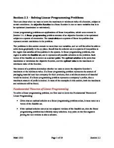
Notice that, in Right Call, the problem to be solved is very similar to the original one: same partial allocation, same stock. This recursive call will trigger a call to the LP routine (call it LP2) solving a LP problem that is very similar to the one just solved (call it LP1). The only difference is that the bid just chosen has disappeared from the list of bids considered by LP2. If this bid did not enter the optimal (fractional) solution of LP1, i.e., if its coefficient in the solution of LP1 was equal to zero, then, the solution of LP2 is the same as that of LP1 and therefore one can save a call to the LP routine. One can easily see that, in this case, no pruning can take place. Figure 1 shows that the saving can be considerable. The auctions are taken from [6]. On the x-axis: the number of bids considered, on the y-axis: under log scale, the number of nodes visited or the number of calls to the LP routine.

3

Experimental Parameters

We ran all our experiments on a Pentium Pro 930 MHz with 512K of memory, running Windows 2000. Our programs were coded in Matlab (R12). We used 5

4

no. of nodes visited and calls

10

3

10

2

10

no. nodes visited no. linprog calls 1

10

0

500

1000

1500

2000

2500

no. of bids

Figure 1: Number of nodes visited vs. Number of calls to the LP routine the linprog facility of the Optimization ToolBox for Linear Programming: this is a primal-dual algorithm. All our results are averages over fifteen auctions drawn from a distribution to be specified for each graph. We did experience some memory problems (probably due to some remaining bugs in Matlab Release 12), but found Matlab extremely easy to use and its linprog facility excellent. The remainder of the paper presents, in graphic form, the results of our experiments. Some of those graphs are difficult to decipher in black and white: we apologize and will produce more readable graphs for the conference paper.

4 4.1

Experimental Results Global Picture

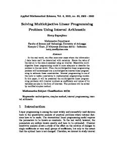
Figure 2 describes the quality of the optimal solution, the lower bound obtained in the initialization phase and two upper bounds for multi-unit auctions. The upper curve (extended norm bound) describes the easy to compute upper bound proposed in [6]. The second (from the top) curve describes the 6

Auction results

upper bound given by Linear Programming. The latter can be proved to be always at most equal to the former. On the x-axis: the number of bids considered (from 250 to 750) and the y-axis the average value (in monetary terms, numbers are not important) of the allocations. This graph shows two things. First, that the lower bound computed in the initialization phase and the upper bound computed by LP are very close. The optimal solution is, obviously, in-between. The larger the auction, the better the convergence of those three values. The second thing is that the easy-to-compute upperbound of [6] is not even close to the LP bound and seems to get (relatively) worse as the number of bids increases. The main claim of this paper is that

Extend norm bound LP bound Greedy approx Optimal 250

300

350

400

450

500 no. of bids

550

600

650

700

750

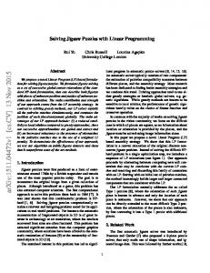
Figure 2: Optimal solution vs. Lower Bound and two Upper Bounds using the time-consuming LP routine is preferable to the use of a lighter but easier to compute upper bound in Bound. Figure 3 compares the running times of the algorithm above that uses LP and the running time of the same algorithm using the easy-to-compute upper bound proposed by LeytonBrown and al. The distribution of auctions is taken from [6], for auctions of different sizes. On the x-axis: the number of bids. On the y-axis: the running time in seconds (log scale). By using LP, one gains two orders of magnitude for large auctions. The lighter upper bound is better for very small numbers of bidders. 7

4

10

3

run time in seconds

10

2

10

1

10

LP bound Extend norm bound 0

10 100

200

300

400

500 600 no. of bids

700

800

900

1000

Figure 3: Running Times using LP vs. Leyton-Brown’s upper bound

5

Initialization Phase

In the initialization phase, in order to find a good solution to be used for pruning, we propose to use many greedy heuristics and keep the best solution found. Figure 4 describes the quality of 16 different greedy heuristics on auctions of varying size (100 to 1000 bids, always 10 goods) taken from the distribution of [6]. On the y-axis: the percentage of the value of the optimal solution reached by the approximation: 100 means perfect approximation, 50 means half of the optimal solution. One expects that criteria that pick up more promising bids first give better results. This is what happens. One sees three main groups. The middle group includes two criteria: picking at random and picking following the (in fact random) order with which bids were given. The lower (worst) group of criteria comprises criteria that choose unattractive bids first. The higher group contains all criteria we thought attractive. It contains both unnormalized and normalized criteria (see [3]). The square-root criterion: p r(a) = qPn

j=1 qj

8

,

(1)

2

approximation ratio (percent

10

sq random original inverse average average average norm inverse sq sq norm inverse euclidean euclidean euclidean norm inverse price price LP inverse LP improved LP

0

200

400

600 no. of bids (10 goods)

800

1000

1200

Figure 4: Value of different greedy heuristics that has been proved to be theoretically optimal, gives the best approximation. The average price per unit gives markedly inferior results. Two criteria based on Linear Programming give pretty good results. The first one solves the relaxed LP problem for the original auction and orders the bids according to their coefficient in the optimal solution, in descending order. The second, improved one, is an adaptative version of the first: it solves a LP problem before choosing each bid (after having eliminated all bids that cannot be granted in full). More on those criteria is found in Section 6.

6

Choosing the bid on which to branch

The main factor in determining the efficiency of our Branch-and-Bound algorithm is the criterion used in choosing the next bid on which to branch in step Choose. Figure 5 compares different such criteria. The graph compares six different criteria. The auctions were taken from [6]. The x-axis shows the number of bids and the y-axis, with a log scale, shows the average number of the nodes visited. The square root criterion of Equation 1 seems best. Nevertheless the LP coefficient criterion and the LP improved criterion 9

4

no. of nodes visited

10

sq criterion price criterion average price criterion size criterion LP coeff criterion LP improved criterion

3

10

100

200

300

400

500 600 no. of bids

700

800

900

1000

Figure 5: Number of nodes visited for different choosing criteria described in Section 5 did very well and even seem better than the square root criterion for large numbers of bids. Figure 6 extends the previous graph to larger auctions, for the best criteria only (for the other criteria we could not finish the search). The criteria based on LP are definitely best.

7

Run Time

We now describe running times for auctions of different sizes, under different distributions. Figure 7 uses the distribution proposed in [6]. Auctions have been generated for 10, 12, 14 and 16 goods. On the x-axis: the number of bids. On the y-axis: running times in seconds (log scale). The curves are sub-linear on a logarithmic scale and exhibit the sub-exponential running time of our algorithm. This graph improves substantially on the similar graph found in [3], showing, again, the advantage of using LP. This graph also shows faster running times for large auctions than the ones presented in [6]. Figure 8 presents similar results for a fixed number of bids (125), for different numbers of goods. The curve is very clearly sub-linear. Contrary to CAMUS, our BB algorithm exhibits a sub-exponential dependence on the 10

4

no. of nodes visited

10

3

10

sq criterion price criterion LP coeff criterion LP improved criterion 2

10 1500

1600

1700

1800

1900

2000 no. of bids

2100

2200

2300

2400

2500

Figure 6: Number of nodes visited for different choosing criteria 3

10

2

run time in seconds

10

1

10

10 goods 12 goods 14 goods 16 goods 0

10

0

500

1000

1500

2000

2500

no. of bids

Figure 7: Running Times for Leyton-Brown and al.’s distribution 11

3

run time in seconds, (over 125 bids)

10

2

10

1

10

0

10

0

20

40

60 no. of goods

80

100

120

Figure 8: Running Times for Leyton-Brown and al.’s distribution number of goods. Figures 9, 10, 11 and 12 describe the running times of our algorithm over four distributions described by de Vries and Vohra [1]. The auctions generated there are single-unit combinatorial auctions. Figure 13 concerns auctions drawn according to the CATS multipaths distribution of the Test Suite in [5]. Notice that our algorithm solves quite easily even auctions with up to 20000 bids. It seems, then, that the CATS multipaths distribution generates problems that are much easier, on average, than those generated by the distribution previously proposed in [6]. This claim is supported by 14. For large numbers of bids, the CATS multipaths distribution indeed generates problems that are easier to solve. There is a simple explanation as to why our BB algorithm solves easily CATS auctions with very large numbers of bids: in fact, one call to the LP routine is typically enough. What happens is that the initialization phase finds an allocation of value v and the first call to the LP routine finds a fractional solution of same value v. This means that the LP fractional problem has an integer solution and the initialization phase found an optimal solution. Our BB algorithm prunes the first node. Figure 15 shows the running times of our algorithm for the distributions of single unit combinatorial auctions suggested by CATS. 12

4

10

100 goods 200 goods 300 goods 400 goods

3

run time in seconds

10

2

10

1

10 500

550

600

650

700

750 no. of bids

800

850

900

950

1000

Figure 9: Running Times for Sandholm Random distribution 3

run time in seconds

10

2

10

100 goods 200 goods 300 goods 400 goods 1

10 500

1000

1500

2000

no. of bids

Figure 10: Running Times for Sandholm Weighted Random distribution 13

2

run time in seconds

10

1

10

25 goods 50 goods 75 goods 100 goods 0

10

50

60

70

80

90 100 110 no. of bids (Uniform Sets = 3)

120

130

140

150

Figure 11: Running Times for Sandholm Uniform distribution: sets of size 3 2

run time in seconds

10

1

10

50 goods 100 goods 150 goods 200 goods 0

10

50

100 150 no. of bids (Alpha in Percent = 55)

200

Figure 12: Running Times for Sandholm Decay distribution: α = 55% 14

3

run time in seconds

10

2

10

1

10

0

2000

4000

6000

8000

10000 no. of bids

12000

14000

16000

18000

Figure 13: Running Times for multipaths distribution 3

10

2

run time in seconds

10

1

10

regular distribution multipaths distribution 0

10

0

500

1000

1500

2000

2500

no. of bids

Figure 14: Relative Difficulty of Leyton-Brown and al.’s distributions 15

1

run time in seconds

10

0

10

my singel distribution arbitrary distribution matching distribution regions distribution scheduling distribution 0

500

1000

1500 no. of bids

2000

2500

Figure 15: Running Time for single-unit CA’s

8

Conclusions

Our first conclusion is that, even though winner determination is theoretically intractable, it can be performed in practice for auctions of a few hundreds goods among a few thousands bids, without a super-computer and without low-level programming optimization. The suggestion of [4] to consider approximately-efficient mechanisms, may have been premature. The challenge is now to tackle auctions of a few thousands goods (such as the FCC auction). But for such situations, the conceptual framework we have worked with in this paper is most probably not adequate: bidders cannot be expected to describe their preferences by an explicit list of bids. Suitable languages for expressing preferences must be found and algorithmic problems studied in such a new framework. Our second conclusion is that the difficulty in solving combinatorial auctions stems more from the number of items for sale than from the number of bids. If the number of bids is large, with respect to the number of items, Linear Programming often finds the optimal integer solution in one call. Our third conclusion is that the method of choosing the next bid on which to branch is extremely important in determining the efficiency of the search. 16

More work is needed to understand what makes a good choice and why the square-root criterion of Equation 1 and the LP adaptative criterion described in Section 6 are so good.

References [1] S. de Vries and R. Vohra. Combinatorial auctions: A survey. http://www.kellogg.nwu.edu/faculty/vohra/htm/res.htm,Test problems at: http://www-m9.mathematik.tu˜ muenchen.de/devries/comb auction supplement/, January 2001. [2] Y. Fujishima, K. Leyton-Brown, and Y. Shoham. Taming the computational complexity of combinatorial auctions: Optimal and approximate approaches. In Proceedings of IJCAI’99, Stockholm, Sweden, July 1999. Morgan Kaufmann. [3] R. Gonen and D. Lehmann. Optimal solutions for multi-unit combinatorial auctions: Branch and bound heuristics. In Second ACM Conference on Electronic Commerce (EC-00), pages 13–20, Minneapolis, Minnesota, October 2000. [4] D. Lehmann, L. I. O’Callaghan, and Y. Shoham. Truth revelation in rapid, approximately efficient combinatorial auctions. In Proceedings of the First ACM Conference on Electronic Commerce. EC’99, pages 96–102, Denver, Colorado, November 1999. SIGecom, ACM Press. [5] K. Leyton-Brown, M. Pearson, and Y. Shoham. Towards a universal test suite for combinatorial auction algorithms. In Proceedings of EC’00, pages 66–76, Minneapolis, Minnesota, October 2000. ACM Press. [6] K. Leyton-Brown, Y. Shoham, and M. Tennenholtz. An algorithm for multi-unit combinatorial auctions. In Proceedings of AAAI, Austin, TX, 2000. [7] N. Nisan. Bidding and allocation in combinatorial auctions. In Proceedings of the 2nd ACM Conference on Electronic Commerce EC’00, pages 1–12, Minneapolis, Minnesota, October 2000. ACM Press.

17

[8] M. H. Rothkopf, A. Pekeˇc, and R. M. Harstad. Computationally manageable combinatorial auctions. Management Science, 44(8):1131–1147, 1998. [9] T. Sandholm. Limitations of the vickrey auction in computational multiagent systems. In 2nd International Conference on Multi-Agent Systems, 1996. [10] T. Sandholm. An algorithm for optimal winner determination in combinatorial auctions. In IJCAI-99, pages 542–547, Stockholm, Sweden, July 1999. [11] T. Sandholm. Approaches to winner determination in combinatorial auctions. Decision Support Systems, 28(1-2):165–176, 2000. [12] T. Sandholm and S. Suri. Improved algorithms for optimal winner determination in combinatorial auctions and generalizations. In Proceedings of the National Conference on Artificial Intelligence (AAAI), Austin, TX, July 1999. [13] M. Tennenholtz. Some tractable combinatorial auctions. Unpublished draft: January 2000.

18