linear regression crash prediction models: issues and ... - MAUTC

LINEAR REGRESSION CRASH PREDICTION MODELS: ISSUES AND PROPOSED SOLUTIONS FINAL REPORT PennDOT/MAUTC Agreement Contract No. 510401 VT-2008-02 DTRS99-G-0003

Prepared for

Virginia Transportation Research Council

By

H. Rakha, M. Arafeh, A. G. Abdel-Salam, F. Guo and A. M. Flintsch

Virginia Tech Transportation Institute May 2010

This work was sponsored by the Virginia Department of Transportation and the U.S. Department of Transportation, Federal Highway Administration. The contents of this report reflect the views of the authors, who are responsible for the facts and the accuracy of the data presented herein. The contents do not necessarily reflect the official views or policies of either the Federal Highway Administration, U.S. Department of Transportation, or the Commonwealth of Virginia at the time of publication. This report does not constitute a standard, specification, or regulation.

1. Report No.

2. Government Accession No.

4. Title and Subtitle LINEAR REGRESSION CRASH PREDICTION MODELS: ISSUES AND PROPOSED SOLUTIONS

3. Recipient’s Catalog No.

5. Report Date May 2010 6. Performing Organization Code

7. Author(s)

8. Performing Organization Report No.

H. Rakha, M. Arafeh, A. G. Abdel-Salam, F. Guo, and A. M. Flintsch

VT-2008-02

9. Performing Organization Name and Address

10. Work Unit No. (TRAIS)

Virginia Tech Transportation Institute 3500 Transportation Research Plaza Blacksburg, VA 24061

11. Contract or Grant No. DTRS99-G-003

12. Sponsoring Agency Name and Address Virginia Department of Transportation ****** U.S. Department of Transportation Research and Innovative Technology Administration UTC Program, RDT-30 1200 New Jersey Ave., SE Washington, DC 20590

13. Type of Report and Period Covered Final Report 14. Sponsoring Agency Code

15. Supplementary Notes

  16. Abstract  The paper develops a linear regression model approach that can be applied to crash data to predict vehicle crashes. The proposed approach involves novice data aggregation to satisfy linear regression assumptions; namely error structure normality and homoscedasticity. The proposed approach is tested and validated using data from 186 access road sections in the state of Virginia. The approach is demonstrated to produce crash predictions consistent with traditional negative binomial and zero inflated negative binomial general linear models. It should be noted however that further testing of the approach on other crash datasets is required to further validate the approach.    17. Key Words

Linear regression model, novice data aggregation, negative binomial, zero inflated negative binomial general linear models.

18. Distribution Statement No restrictions. This document is available from the National Technical Information Service, Springfield, VA 22161

19. Security Classif. (of this report)

20. Security Classif. (of this page)

21. No. of Pages

Unclassified

Unclassified

21

Form DOT F 1700.7 authorized

(8-72)

22. Price

Technical Report Documentation Page Reproduction of completed page

TABLE OF CONTENTS Introduction .................................................................................................................................... 1 Background .................................................................................................................................... 1 Data Description ............................................................................................................................ 2 Model Development....................................................................................................................... 3 Summary Findings ....................................................................................................................... 19

LIST OF FIGURES Figure 1. Effect of Access Section Length within AADT Binning .............................................. 6 Figure 2. Test of Normality of AADT Adjustment Factors.......................................................... 7 Figure 3. Computation of Exposure Measure ............................................................................... 7 Figure 4. Test of Normality for Crash Rate Data......................................................................... 8 Figure 5. Crash Prediction Model Considering Nearest Access Point ........................................ 9 Figure 6. Crash Prediction Model Considering Nearest Intersection ........................................ 10 Figure 7. Variation in Expected Crashes as a Function of AADT Exponent ............................ 11 Figure 8. Variation in the Expected Number of Yearly Crashes as a Function of the Access Section Length and AADT ............................................................................ 12 Figure 9. Variation in Expected Crashes/Km as a Function of AADT Exponent .................... 13 Figure 10. Variation in the Expected Number of Yearly Crashes per Kilometer as a Function of the Access Section Length and AADT................................................. 14 Figure 11. Comparison of Actual and Expected Crashes over a 5-year Period (All 186 Sites) ....................................................................................................................... 15

v

LIST OF TABLES Table 1. Summary Results of Regression Models ........................................................................ 4 Table 2. Impact of Access Road Spacing on Annual Crash Rate (AADT = 20,000 veh/day) ... 16

vi

vi

Linear regression crash prediction models: issues and proposed solutions H. Rakha Charles Via, Jr. Department of Civil and Environmental Engineering, Blacksburg, Virginia, USA

M. Arafeh, A.G. Abdel-salam, F. Guo and A.M. Flintsch Virginia Tech Transportation Institute, Blacksburg, Virginia,USA

ABSTRACT: The paper develops a linear regression model approach that can be applied to crash data to predict vehicle crashes. The proposed approach involves novice data aggregation to satisfy linear regression assumptions; namely error structure normality and homoscedasticity. The proposed approach is tested and validated using data from 186 access road sections in the state of Virginia. The approach is demonstrated to produce crash predictions consistent with traditional negative binomial and zero inflated negative binomial general linear models. It should be noted however that further testing of the approach on other crash datasets is required to further validate the approach. INTRODUCTION The current state-of-the-art for developing Crash Prediction Models (CPMs) is to adopt General Linear Models (GLMs) considering either a Poisson or a negative binomial error structure (Lord et al. 2004; Lord et al. 2005; Sawalha et al. 2006). Recently, researchers have also proposed the use of zero inflated negative binomial regression models in order to address the high propensity of zero crashes within typical crash data (Shankar et al. 1997; Shankar et al. 2003). The use of Linear Regression Models (LRMs) is not utilized because crash data typically do not satisfy the assumptions of such models, namely: normal error structure and constant error variance. The objectives of the research presented in this paper are two-fold. First, the paper demonstrates how through the use of data manipulation it is possible to satisfy the assumptions of LRMs and thus develop robust LRMs. Second, the paper compares the LRM approach to the traditional GLM approach considering a negative binomial error structure to demonstrate the adequacy of the proposed approach. The objectives of the paper are achieved by applying the models to crash, traffic, and roadway geometric data obtained from 186 freeway access roads in the state of Virginia in the U.S. In terms of the paper layout, initially a brief background of CPMs is presented. Subsequently, the unique characteristics of the crash, traffic, and roadway geometry data that are utilized to validate the proposed approach are described. Next, the two modeling approaches are described and applied to the access road data. Finally, the study conclusions are presented. BACKGROUND An earlier publication (Lord et al. 2004) indicated that “there has been considerable research conducted over the last 20 years focused on predicting motor vehicle crashes on transportation facilities. The range of statistical models commonly applied includes binomial, Poisson, Poisson-gamma (or Negative Binomial), Zero-Inflated Poisson and Negative Binomial Models (ZIP and ZINB), and Multinomial probability models. Given the range of possible modeling

approaches and the host of assumptions with each modeling approach, making an intelligent choice for modeling motor vehicle crash data is difficult at best.” The authors further indicate that “in recent years, some researchers have applied “zero-inflated” or “zero altered” probability models, which assume that a dual-state process is responsible for generating the crash data.” The authors indicated that “these models have been applied to capture the ‘excess’ zeroes that commonly arise in crash data—and generally have provided improved fit to data compared to Poisson and Negative Binomial (NB) regression models.” Lord et al. (Lord et al. 2004) conducted a simulation experiment to demonstrate how crash data may give rise to “excess” zeroes. They demonstrated that under certain (fairly common) circumstances excess zeroes are observed—and that these circumstances arise from low exposure and/or inappropriate selection of time/space scales and not an underlying dual state process. They concluded that a careful selection of the time/space scales for analysis, including an improved set of explanatory variables and/or unobserved heterogeneity effects in count regression models, or applying small area statistical methods (observations with low exposure) represent the most defensible modeling approaches for datasets with a preponderance of zeros. We partially agree with these conclusions, however modelers my not have much choice in their time/space scale selection given the limitation of traffic and crash data. In this paper we present an alternative approach that combines novice data aggregation with LRMs to address the challenges of crash data that were described earlier. DATA DESCRIPTION As was mentioned earlier, the two approaches for developing CPMs are demonstrated using a database of crash, traffic, and geometric data obtained from 186 randomly selected arterial access roads connected to freeway ramps. The sections that were considered included the following: 1. Areas designated as rural (79 observations) and others designated as urban (107 observations), 2. Sections with (76 observations) and without acceleration lanes (110 observations), 3. Arterial facilities with a median (121 observations) versus without (65 observations), 4. With 2, 4, or 6 lanes (57, 95, and 34 observations, respectively), 5. First intersection either signalized, stop-sign controlled, or no control on the arterial, and 6. Sections with a left turn bay (78 observations) versus without (108 observations). The length of the access roads varied from 3 to 1110 m with an average length of 169 m while the distance to the first intersection varied from 6 to 2285 m with an average value of 298 m. The Average Annual Daily Traffic (AADT) varied from 112 to 117,314 with an average AADT of 19,456 veh/day. The number of crashes over 5 years varied from 0 to 169 crashes in a section with an average number of crashes of 12 over the 186 study sections. The crash data were extracted from the Highway Traffic Records Information System Crash Database (HTRIS) for the years 2001 through 2005. The traffic data were obtained from the Road inventory VDOT database. The data represents the AADT of the section with a few exceptions were the traffic data represent a 24 hour count.

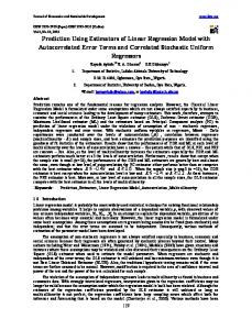
After fusing the crash, traffic, and geometric data it was possible to plot the data, as illustrated in Error! Reference source not found.. Specifically, the figure demonstrates a general increase 200 Crashes

150 100 50 0 12

10

4

x 10

8

6

4

AADT (veh/day)

2

0

0.2

0

0.6

0.4

0.8

1.4

1.2

1

Distance to First Access (km)

70 60

Frequency

50 40 30 20 10 0

0

20

40

60

80

100

120

140

160

180

Crashes

in the number of crashes as the facility Average Annual Daily Traffic (AADT) increases. The figure also illustrates a high cluster of data at the short access road distances with minimum observations for access roads in excess of 400 m. Similarly, AADTs in excess of 8,000 veh/day are a rare occurrence. The figure does illustrate a number of sections with high AADTs and short access roads with a small number of crashes. Conversely, observations with high crashes are also observed for low AADTs and long access roads. Figure 1. Data Distribution.

The crash frequency distribution demonstrates that the number of crashes ranges from a minimum of 0 to a maximum of 169 crashes over 5 years, as illustrated in Error! Reference source not found.. The higher frequency of zero crashes is typical of crash data when the exposure rate is low as was described in the literature (Lord et al. 2004). The higher propensity of zero observations has lead some researchers to apply zero-inflated negative binomial models to the modeling of crashes considering two underlying processes (Shankar et al. 1997; Shankar et al. 2003). The frequency distribution is consistent with a negative binomial distribution with a consistent decrease in the frequency as the number of crashes increases. A statistical analysis of the data demonstrated that the type of road (rural versus urban), number of lanes, the availability of a median, the type of signal control at the nearest intersection, and availability of an acceleration lane were not statistically significant. The details of these statistical tests are beyond the scope of this paper, but are provided elsewhere (Medina Flintsch et al. 2008). MODEL DEVELOPMENT This section describes the two approaches that were tested in the paper for developing crash prediction models. The first approach is the common approach that is reported in the literature, which is based on the use of Poisson, Negative Binomial (NB), Zero Inflated Poisson (ZIP), and Zero Inflated Negative Binomial (ZINB) regression models. An alternative approach that is developed in this paper is the use of LRMs. Initially, a discussion of the NB and ZINB

regression approach is presented followed by a discussion of the proposed LRM approach. Both approaches are then compared using crash data from 186 access roads in the state of Virginia in the U.S. Prior to describing the various models, the model structure is discussed. Specifically, the study considers a crash rate that is formulated as CR =

C 106 ⋅ = exp ( β0 + β1L1 ) , L2V p ( 365 × 5 )p

[1]

where CR is the crash rate (million vehicle crashes per vehicle kilometer of exposure over a 5 year period), C is the total number of crashes over the study section of length L2 in the 5-year analysis period (crashes), L2 is the length of the section which is the distance between the freeway off-ramp and the first intersection (km), L1 is the distance between the freeway offramp and the first access road (may equal L2 if the first access road is an intersection) (km), V is the section AADT (veh/day), B0 and B1 are the model constants. The model of Equation [1] can then be manipulated to produce a linear model of the form p

C =

( 365 × 5 ) 106

⋅ exp ( β0 + β1L1 + ln(L2 ) + p ln(V ) ) + E

.

[2]

Here E is a random error term that accounts for the error that is not captured in the model. The advantage of this model is that (a) it is linear in structure after applying a logarithmic transformation; (b) it ensures that the crashes are positive (greater than or equal to zero); and (c) it produces zero crashes when the exposure is set to zero (i.e. when L2 or V is zero). Poisson or Negative Binomial Model Approach The Poisson distribution is more frequently applied to models with count data. The probability mass function of a Poisson crash random variable (λ is the mean crashes per unit time) is given by P (C ) =

λC −C e ; C = 0,1,... C!

[3]

One feature of the Poisson random variable (C) is the identity of the mean and variance. The NB model overcomes this limitation by considering the λ parameter to be a random variable that is distributed following a Poisson distribution. Consequently, the negative binomial distribution has the same support (C=0,1,2, …) as the Poisson distribution but allows for greater variability within the data (variance can be greater than the mean). Consequently, a good alternative model for count data that exhibit excess variation compared to a Poisson model is the negative binomial model. The structure of the GLM model that computes the expected number of crashes (E(C) can be written as p ⎞ ⎛ ⎜ ( 365 × 5 ) ⎟⎟ ⎟⎟ L2 ⋅ exp ( β0 + β1L1 + p ln(V ) ) . E (C ) = ⎜⎜⎜ ⎟⎟ 6 ⎜⎜ 10 ⎟⎠ ⎝

[4]

Two sets of Poisson and two NB models were developed, one a standard model (NB and Poisson) and one a zero inflated model (ZINB and ZIP), as summarized in Table 1. Unfortunately, the Poisson regression model suffered from over-dispersion as indicated by the value of the deviance divided by the degrees of freedom which was much greater than a value of 1.0 (was 184.7). Consequently, a Modified Poisson Regression was also applied using an overdispersion parameter. The model produces the same parameter values; however, the deviance is reduced to 1.0 and thus is valid from a statistical standpoint. In the case of the NB model the value of the deviance divided by the degrees of freedom was close to a value of 1.0 (1.2063) and

thus demonstrating the adequacy of the negative binomial error structure. It should be noted that the model predictions for the zero-inflated models are computed my multiplying the results of Equation [4] by 1 − exp(θ) ( 1 + exp(θ) ) as p ⎞ ⎛ ⎜ ( 365 × 5 ) ⎟⎟ ⎛ ⎞ ⎟⎟ L2 ⋅ exp ( β0 + β1L1 + p ln(V ) ) × ⎜⎜ 1 − exp(θ) ⎟⎟ . E (C ) = ⎜⎜⎜ ⎜ ⎜⎜ ⎝ 1 + exp(θ) ⎟⎟⎠ ⎟⎟⎟⎠ 106 ⎝

[5]

Table 1: Summary Results of Regression Models Parameter

LRM

NB

Poisson

ZINB

ZIP

B0

4.27

4.76

3.42

4.76

3.83

B1

-6.88

-3.64

-6.90

-3.64

-2.00

p

0.86

0.81

0.92

0.81

0.84

θ

0.00

0.00

0.00

-16.00

-1.69

365608

389589

437926

389589

254307

SSE SSE (%) Slope Error (%)

0%

7%

20%

7%

-30%

0.472

0.512

0.549

0.512

0.339

2.12

1.95

1.82

1.95

2.95

The results of Table 1 demonstrate that the model parameters a practically identical for both the NB and ZINB models except for the θ parameter. Given that the θ parameter is much less than zero the predictions of the NB and ZINB are very similar. In the case of the Poisson models (Poisson and ZIP) the model parameter values are significantly different, as demonstrated in Table 1. Linear Regression Modeling Approach In this section we consider a linear regression approach for the development of a model. If we consider the number of crashes per unit distance as our dependent variable the model of Equation [2] can be cast as p

( 365 × 5 ) E(C ) = E(C ′) = ⋅ exp ( β0 + β1L1 + p ln(V ) ) . L2 106

[6]

Equation [6] is a linear model with two independent variables: V and L1. It should be noted that an analysis of crashes per unit distance ensures that the data are normalized across the different section lengths. The development of a LRM using the least squares approach requires that the data follow a normal distribution. A statistical analysis of the data revealed that there was insufficient evidence to conclude that the data were normal. Furthermore, the dispersion parameter, which measures the amount of variation in the data, was significantly greater than 1.0 indicating that a negative binomial model would be appropriate for the data. Here we present an approach for normalizing the data in order to apply a least squared LRM to the data. The approach involves sorting the data based on one of the independent variables and then aggregating the data using a variable bin size to ensure that the second independent variable remains constant across the various bins. Data transformations can then be applied to the data to ensure normality and homoscedasticity (equal variance). Once the parameters of the first independent variable are computed, the data are sorted on the second independent variable. The data are then aggregated in order to ensure normality and homoscedasticity and then linear models are fit to the data to compute the variable coefficient. The approach is demonstrated using the access road crash data in the following sub-sections. Selecting Exposure Measures The typical exposure measure for crashes is million vehicle-miles or million vehicle-kilometers of travel. However, researchers have argued that the exponent of the volume variable (V) in the exposure measure is not necessarily equal to 1.0 [7, 8]. Consequently, the first step in the analysis was to compute the exponent of V (denoted as p).

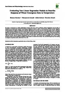
Given that the data vary as a function of two variables L1 and V, it was important to normalize one of the variables while analyzing the second variable. In order to estimate the volume exponent, the data were sorted based on their AADT values and aggregated using variable bin sizes to ensure that the L1 variable remained constant across the various bins, as illustrated in Figure 1. The figure demonstrates that by performing a linear regression of L1 against V that the slope of the line is insignificant (p > 0.05) and thus there is insufficient evidence to conclude that the L1 variable varies across the aggregated data. 250

Regression Statistics R2 0.509 R2 (Adj) 0.386 Obs. 6

Length (m)

200 150

ANOVA df

100

Reg. Residual Total

50 0 0

20000

40000 AADT

60000

80000

Intercept AADT

SS MS 1 17608.38 17608.38 4 17003.46 4250.86 5 34611.84

Coeff. 530.039 0.002

SE 35.820 0.001

F 4.14

ignificance F 0.11

t Stat P-value Low 95% Up 95% 14.80 0.00 430.59 629.49 2.04 0.11 0.00 0.01

Figure 1. Effect of Access Section Length within AADT Binning.

In estimating crash rates it is important that the measure of exposure ensures that the data are normalized. In doing so a multiplicative crash adjustment factor (Fi) for each bin i was computed as ⎡ ⎛ C ij min ⎢ max ⎜⎜ i ⎢ j ⎜ ⎝ Lij ⎣ Fi = ⎛ C ij ⎞⎟ max ⎜⎜ ⎟ j ⎜ ⎝ Lij ⎟⎠

⎞⎤ ⎟⎟ ⎥ ⎟⎠ ⎥ ⎦

,

[7]

where Cij is the number of crashes for section j in bin i and Lij is the length of section j in bin i. The Fi correction factor ensures that the maximum number of crashes remains constant (equal to the minimum number of crashes) across the various bins, which is by definition what an exposure measure is. The correction factor is also equal to Fi = αViβ ,

[8]

where Vi is the mean AADT volume across all observations j in bin i and α and β are model coefficients. By solving Equation [7] and [8] simultaneously we derive ⎛ C ij CR = Fi ⋅ max ⎜⎜ ⎜ Lij j ⎝

⎞⎟ ⎛ C ij ⎟ = αViβ ⋅ max ⎜⎜ ⎜ Lij j ⎝ ⎠⎟

⎞⎟ Ci Crashes . = ⎟= α⋅ −β Length ⋅ AADT p ⎠⎟ LV i i

[9]

Consequently, β is equivalent to -p and can be solved for by fitting a regression line to the logarithmic transformation of Equation [8] as ln ( Fi ) = ln ( α ) + β ln (Vi ) .

[10]

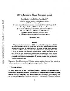
After applying a least squared fit to the data, the model residual errors were tested for normality. As illustrated in Figure 2, although in the case of the original non-transformed data the residual error did not pass the normality test, the log-transformed residual errors did pass the test (p = 0.355).

99

99

Mean StDev N AD P-Value

95 90

90

70

60

60

50 40

40 30

20

20

10

10

5

5

-1.0

8.511710E-16 0.5273 6 0.340 0.355

50

30

1

Mean StDev N AD P-Value

80

70

Percent

Percent

80

95

-9.71445E-17 0.3378 6 0.684 0.036

-0.5

0.0 Residuals of F

0.5

1

1.0

(a) Normality Test on Fi

-1.0

-0.5

0.0 0.5 Residual of Ln(F)

1.0

(b) Normality Test on Log-transformed Fi

Figure 2. Test of Normality of AADT Adjustment Factors.

A least squares LRM was then fit to the log-transformed data producing an R2 of 0.89, as illustrated in Figure 3. The model was statistically significant (p