Linear scale-space

Linear scale-space

by Tony Lindeberg

Royal Institute of Technology (KTH) Computational Vision and Active Perception Laboratory (CVAP) Department of Numerical Analysis and Computing Science S-100 44 Stockholm, Sweden and Bart M. ter Haar Romeny

Utrecht University, Computer Vision Research Group, Heidelberglaan 100 E.02.222, NL-3584 CX Utrecht, The Netherlands To appear in Geometry-Driven Diusion in Computer Vision , (ter Haar Romeny, ed.) Kluwer Academic Publishers, Series in Mathematical Imaging and Vision, Dordrecht, Netherlands, 1994.

Contents \Linear scale-space I: Basic theory" \Linear scale-space II: Early visual operations"

i

pp. 1{41 pp. 43{77

ii

Table of Contents 0 1 LINEAR SCALE-SPACE I: BASIC THEORY

Tony Lindeberg and Bart M. ter Haar Romeny 1.1 Introduction : : : : : : : : : : : : : : : : : : : : : : : : 1.1.1 Early visual operations : : : : : : : : : : : : : 1.2 Multi-scale representation of image data : : : : : : : : 1.3 Early multi-scale representations : : : : : : : : : : : : 1.3.1 Quad tree : : : : : : : : : : : : : : : : : : : : : 1.3.2 Pyramids : : : : : : : : : : : : : : : : : : : : : 1.4 Linear scale-space : : : : : : : : : : : : : : : : : : : : : 1.5 Towards formalizing the scale-space concept : : : : : : 1.5.1 Continuous signals: Original formulation : : : : 1.5.2 Inner scale, outer scale, and scale-space : : : : 1.5.3 Causality : : : : : : : : : : : : : : : : : : : : : 1.5.4 Non-creation of local extrema : : : : : : : : : : 1.5.5 Semi-group and continuous scale parameter : : 1.5.6 Scale invariance and the Pi theorem : : : : : : 1.5.7 Other special properties of the Gaussian kernel 1.6 Gaussian derivative operators : : : : : : : : : : : : : : 1.6.1 In nite dierentiability : : : : : : : : : : : : : 1.6.2 Multi-scale N -jet representation and necessity : 1.6.3 Scale-space properties of Gaussian derivatives : 1.6.4 Directional derivatives : : : : : : : : : : : : : : 1.7 Discrete scale-space : : : : : : : : : : : : : : : : : : : : 1.7.1 Non-creation of local extrema : : : : : : : : : : 1.7.2 Non-enhancement and in nitesimal generator : 1.7.3 Discrete derivative approximations : : : : : : : 1.8 Scale-space operators and front-end vision : : : : : : : 1.8.1 Scale-space: A canonical visual front-end model 1.8.2 Relations to biological vision : : : : : : : : : :

iii

i 1 : : : : : : : : : : : : : : : : : : : : : : : : : : :

: : : : : : : : : : : : : : : : : : : : : : : : : : :

: : : : : : : : : : : : : : : : : : : : : : : : : : :

1 3 3 5 6 6 10 13 13 14 15 16 17 18 24 25 25 25 28 29 29 30 33 35 35 36 36

iv

CHAPTER 0

1.8.3 Foveal vision : : : : : : : : : : : : : : : : : : : : : : 37

2 LINEAR SCALE-SPACE II: EARLY VISUAL OPERATIONS 39 Tony Lindeberg and Bart M. ter Haar Romeny 2.1 Introduction : : : : : : : : : : : : : : : : : : : : : : : : : : 2.2 Multi-scale feature detection in scale-space : : : : : : : : : 2.2.1 Dierential geometry and dierential invariants : : 2.2.2 Feature detection from dierential singularities : : 2.2.3 Scale selection : : : : : : : : : : : : : : : : : : : : 2.2.4 Cues to surface shape (texture and disparity) : : : 2.3 Behaviour across scales: Deep structure : : : : : : : : : : 2.3.1 Iso-intensity linking : : : : : : : : : : : : : : : : : 2.3.2 Feature based linking (dierential singularities) : : 2.3.3 Bifurcations in scale-space : : : : : : : : : : : : : : 2.4 Scale sampling : : : : : : : : : : : : : : : : : : : : : : : : 2.4.1 Natural scale parameter: Eective scale : : : : : : 2.5 Regularization properties of scale-space kernels : : : : : : 2.6 Related multi-scale representations : : : : : : : : : : : : : 2.6.1 Wavelets : : : : : : : : : : : : : : : : : : : : : : : : 2.6.2 Tuned scale-space kernels : : : : : : : : : : : : : : 2.7 Behaviour across scales: Statistical analysis : : : : : : : : 2.7.1 Decreasing number of local extrema : : : : : : : : 2.7.2 Noise propagation in scale-space derivatives : : : : 2.8 Non-uniform smoothing : : : : : : : : : : : : : : : : : : : 2.8.1 Shape distortions in computation of surface shape. 2.8.2 Outlook : : : : : : : : : : : : : : : : : : : : : : : :

References Index

: : : : : : : : : : : : : : : : : : : : : :

39 40 40 44 50 53 55 55 56 58 59 59 60 61 61 62 64 64 66 67 68 70

73 80

LINEAR SCALE-SPACE I: BASIC THEORY Tony Lindeberg

Royal Institute of Technology (KTH) Computational Vision and Active Perception Laboratory (CVAP) Department of Numerical Analysis and Computing Science S-100 44 Stockholm, Sweden and

Bart M. ter Haar Romeny

Utrecht University, Computer Vision Research Group, Heidelberglaan 100 E.02.222, NL-3584 CX Utrecht, The Netherlands

1.1. Introduction Vision deals with the problem of deriving information about the world from the light re ected from it. Although the active and task-oriented nature of vision is only implicit in this formulation, this view captures several of the essential aspects of vision. As Marr (1982) phrased it in his book Vision, vision is an information processing task, in which an internal representation of information is of out-most importance. Only by representation information can be captured and made available to decision processes. The purpose of a representation is to make certain aspects of the information content explicit , that is, immediately accessible without any need for additional processing. This introductory chapter deals with a fundamental aspect of early image representation|the notion of scale . As Koenderink (1984) emphasizes, the problem of scale must be faced in any imaging situation. An inherent property of objects in the world and details in images is that they only exist as meaningful entities over certain ranges of scale. A simple example of this is the concept of a branch of a tree, which makes sense only at a scale from, say, a few centimeters to at most a 1

2

1. Linear scale-space: Basic theory

few meters. It is meaningless to discuss the tree concept at the nanometer or the kilometer level. At those scales it is more relevant to talk about the molecules that form the leaves of the tree, or the forest in which the tree grows. Consequently, a multi-scale representation is of crucial importance if one aims at describing the structure of the world, or more speci cally the structure of projections of the three-dimensional world onto two-dimensional images. The need for multi-scale representation is well understood, for example, in cartography; maps are produced at dierent degrees of abstraction. A map of the world contains the largest countries and islands, and possibly, some of the major cities, whereas towns and smaller islands appear at rst in a map of a country. In a city guide, the level of abstraction is changed considerably to include streets and buildings etc. In other words, maps constitute symbolic multi-scale representations of the world around us, although constructed manually and with very speci c purposes in mind. To compute any type of representation from image data, it is necessary to extract information, and hence interact with the data using certain operators . Some of the most fundamental problems in low-level vision and image analysis concern: what operators to use, where to apply them, and how large they should be. If these problems are not appropriately addressed, the task of interpreting the output results can be very hard. Ultimately, the task of extracting information from real image data is severely in uenced by the inherent measurement problem that real-world structures, in contrast to certain ideal mathematical entities, such as \points" or \lines", appear in dierent ways depending upon the scale of observation. Phrasing the problem in this way shows the intimate relation to physics. Any physical observation by necessity has to be done through some nite aperture , and the result will, in general, depend on the aperture of observation. This holds for any device that registers physical entities from the real world including a vision system based on brightness data. Whereas constant size aperture functions may be sucient in many (controlled) physical applications, e.g., xed measurement devices, and also the aperture functions of the basic sensors in a camera (or retina) may have to determined a priori because of practical design constraints, it is far from clear that registering data at a xed level of resolution is sucient. A vision system for handling objects of dierent sizes and at dierence distances needs a way to control the scale(s) at which the world is observed. The goal of this chapter is to review some fundamental results concerning a framework known as scale-space that has been developed by the computer vision community for controlling the scale of observation and representing the multi-scale nature of image data. Starting from a set of basic constraints (axioms) on the rst stages of visual processing it will

Lindeberg and ter Haar Romeny

3

be shown that under reasonable conditions it is possible to substantially restrict the class of possible operations and to derive a (unique) set of weighting pro les for the aperture functions. In fact, the operators that are obtained bear qualitative similarities to receptive elds at the very earliest stages of (human) visual processing (Koenderink 1992). We shall mainly be concerned with the operations that are performed directly on raw image data by the processing modules are collectively termed the visual front-end. The purpose of this processing is to register the information on the retina, and to make important aspects of it explicit that are to be used in later stage processes. If the operations are to be local, they have to preserve the topology at the retina; for this reason the processing can be termed retinotopic processing.

1.1.1. Early visual operations An obvious problem concerns what information should be extracted and what computations should be performed at these levels. Is any type of operation feasible? An axiomatic approach that has been adopted in order to restrict the space of possibilities is to assume that the very rst stages of visual processing should be able to function without any direct knowledge about what can be expected to be in the scene. As a consequence, the rst stages of visual processing should be as uncommitted and make as few irreversible decisions or choices as possible. The Euclidean nature of the world around us and the perspective mapping onto images impose natural constraints on a visual system. Objects move rigidly, the illumination varies, the size of objects at the retina changes with the depth from the eye, view directions may change etc. Hence, it is natural to require early visual operations to be unaected by certain primitive transformations (e.g. translations, rotations, and greyscale transformations). In other words, the visual system should extract properties that are invariant with respect to these transformations. As we shall see below, these constraints leads to operations that correspond to spatio-temporal derivatives which are then used for computing (dierential) geometric descriptions of the incoming data ow. Based on the output of these operations, in turn, a large number of feature detectors can be expressed as well as modules for computing surface shape. The subject of this chapter is to present a tutorial overview on the historical and current insights of linear scale-space theories as a paradigm for describing the structure of scalar images and as a basis for early vision. For other introductory texts on scale-space; see the monographs by Lindeberg (1991, 1994) and Florack (1993) as well as the overview articles by ter Haar Romeny and Florack (1993) and Lindeberg (1994).

4


1.2. Multi-scale representation of image data Performing a physical observation (e.g. looking at an image) means that some physical quantity is measured using some set (array) of measuring devices with certain apertures. A basic tradeo problem that arises in this context is that if we are interested in resolving small details then the apertures should be narrow which means that less of the physical entity will be registered. A larger aperture on the other hand gives a stronger response and coarser details. Since we, in general, cannot know in advance what aperture sizes are appropriate, we would like to be able to treat the scale of observation as a free parameter so as to be able to handle all scales simultaneously. This concept of having a range of measurements using apertures of dierent physical sizes corresponding to observations at a range of scales is called a multi-scale measurement of data.

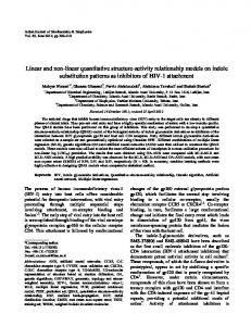
increasing t

coarser levels of scale original signal

Figure 1.1. A multi-scale representation of a signal is an ordered set of derived signals intended to represent the original signal at various levels of scale. (From [76].)

In case a set of measurement data is already given (as is the case when an image is registered at a certain scale using a camera) this process can be simulated by the vision system. The basic idea behind a multi-scale representation is to embed the original signal into such a one-parameter family of derived signals. How should such a representation be constructed? A crucial requirement is that structures at coarse scales in the multi-scale representation should constitute simpli cations of corresponding structures at ner scales|they should not be accidental phenomena created by the smoothing method. This property has been formalized in a variety of ways by dierent authors. A noteworthy coincidence is that the same conclusion can be reached from several dierent starting points. The main result we shall


5

arrive at is that if rather general conditions are imposed on the types of computations that are to be performed at the rst stages of visual processing, then the Gaussian kernel and its derivatives are singled out as the only possible smoothing kernels. The requirements, or axioms, that specify the Gaussian kernel are basically linearity and spatial shift invariance combined with dierent ways of formalizing the notion that structures at coarse scales should be related to structures at ner scales in a well-behaved manner; new structures should not be created by the smoothing method. An simple example where structure is created in a \multi-scale representation" is when an image is enlarged by pixel replication (see gure 1.2). The sharp boundaries at regular distances are not present in the original data; they are just artifacts of the scale-changing (zooming) process.

Figure 1.2. Example of what may be called creation of spurious structure; here by generating coarser-scale image representations by subsampling followed by pixel replication. (left) Magnetic resonance image of the cortex at resolution 240 80 pixels. (middle) Subsampled to a resolution of 48 16 pixels and illustrated by pixel replication. (right) Subsampled to 48 16 pixels and illustrated by Gaussian interpolation.

Why should one represent a signal at multiple scales when all information is present in the original data anyway? The major reason for this is to explicitly represent the multi-scale aspect of real-world images1 . Another aim is to simplify further processing by removing unnecessary and disturbing details. More technically, the latter motivation re ects the common need for smoothing as a pre-processing step to many numerical algorithms as a means of noise suppression. Of course, there exists a large number of possible ways to construct a one-parameter family of derived signals from a given signal. The terminology that will be adopted2 here is to refer to as a \multi-scale representation" any one-parameter family for which the parameter has a clear interpretation in terms of spatial scale. 1 At the rst stages there should be no preference for any certain scale or range of

scales; all scales should be measured and represented equivalently. In later stages the task may in uence the selection, for example, do we want to see the tree or the leaves? 2 In some literature the term \scale-space" is used for denoting any type of multi-scale representation. Using that terminology, the scale-space concept developed here should be called \(linear) diusion scale-space".

6


1.3. Early multi-scale representations The general idea of representing a signal at multiple scales is not entirely new. Early work in this direction was performed by e.g. Rosenfeld and Thurston (1971), who observed the advantage of using operators of dierent size in edge detection. Related approaches were considered by Klinger (1971), Uhr (1972), Hanson and Riseman (1974), and Tanimoto and Pavlidis (1975) concerning image representations using dierent levels of spatial resolution, i.e., dierent amounts of subsampling. These ideas have then been furthered, mainly by Burt and by Crowley, to one of the types of multi-scale representations most widely used today, the pyramid . A brief overview of this concept is given below.

1.3.1. Quad tree One of the earliest types of multi-scale representations of image data is the quad tree 3 introduced by Klinger (1971). It is a tree-like representation of image data in which the image is recursively divided into smaller regions. The basic idea is as follows: Consider, for simplicity, a discrete twodimensional image I of size 2K 2K for some K 2 N, and de ne a measure of the grey-level variation in any region. This measure may e.g. be the standard deviation of the grey-level values. Let I (K ) = I . If (I (K )) is greater than some pre-speci ed threshold , then split I (K ) into sub-images Ij(K ;1) (j = 1::p) according to a speci ed rule. Apply this procedure recursively to all sub-images until convergence is obtained. A tree of degree p is generated, in which each leaf Ij(k) is a homogeneous block with (Ij(k)) < . (One example is given in gure 1.3.) In the worst case, each pixel may correspond to an individual leaf. On the other hand, if the image contains a small number of regions with relatively uniform grey-levels, then a substantial data reduction can be obtained. This representation has been used in simple segmentation algorithms for image processing of grey-level data. In the \split-and-merge" algorithm, a splitting step is rst performed according to the above scheme. Then, adjacent regions are merged if the variation measure of the union of the two regions is below the threshold. Another application (when typically = 0) concerns objects de ned by uniform grey-levels, e.g. binary objects; see e.g. the book by Tanimoto and Klinger (1980) for more references on this type of representation. 3 For three-dimensional data sets, the corresponding representation is usually referred to as octtree .


7

Figure 1.3. Illustration of quad-tree and the split-and-merge segmentation algorithm; (left) grey-level image, (middle) the leaves of the quad-tree, i.e., the regions after the split step that have a standard deviation below the given threshold, (right) regions after the merge step. (From [76].)

1.3.2. Pyramids Pyramids are representations that combine the subsampling operation with a smoothing step. Historically they have yielded important steps towards current scale-space theories and we shall therefore consider them in more detail. To illustrate the idea, assume again, for simplicity, that the size of the input image I is 2K 2K , and let I (K ) = I . The representation of I (K ) at a coarser level I (K ;1) is de ned by a reduction operator. Moreover, assume that the smoothing lter is separable, and that the number of lter coecients along one dimension is odd. Then, it is sucient to study the following one-dimensional situation:

f (k;1) = REDUCE( f (k)) PN ( k ; 1) f (x) = n=;N c(n) f (k)(2x ; n);

(1.1)

where c: Z ! R denotes a set of lter coecients. This type of lowpass pyramid representation (see gures 1.4{1.5) was proposed almost simultaneously by Burt (1981) and in a thesis by Crowley (1981). Low-pass and band-pass pyramids: Basic structure. A main advantage of this representation is that the image size decreases exponentially with the scale level, and hence also the amount of computations required to process the data. If the lter coecients c(n) are chosen properly, the representations at coarser scale levels (smaller k) will correspond to coarser scale structures in the image data. How can the lter be determined? Some of the most obvious design criteria that have been proposed for determining the lter coecients are: ; positivity: c(n) 0,

8


2n;1 2n;1 2n 2n

2n+1 2n+1 Figure 1.4. A pyramid representation is obtained by successively reducing the image size by combined smoothing and subsampling. (From [76].)

; unimodality: c(jnj) c(jn + 1j), ; symmetry: c(;n)N= c(n), and ; normalization: n=;N c(n) = 1. P

Another natural condition is that all pixels should contribute equally to all levels. In other words, any point that has an odd coordinate index should contribute equally to the next coarser level as any point having an even coordinate value. Formally this can be expressed as ; equal contribution: PNn=;N c(2n) = PNn=;N c(2n + 1). Equivalently, this condition means that the kernel (1=2; 1=2) of width two should occur as at least one factor in the smoothing kernel. The choice of the lter size N gives rise to a trade-o problem. A larger value of N increases the number of degrees of freedom in the design at the cost of increased computational work. A natural choice when N = 1 is the binomial lter (1; 1; 1) (1.2) 4 2 4 which is the unique lter of width three that satis es the equal contribution condition. It is alsoPthe unique lter of width three for which the Fourier transform () = Nn=;N c(n) exp(;in) is zero at = . A negative property of this kernel, however, is that when applied repeatedly, the equivalent convolution kernel (which corresponds to the combined eect of iterated smoothing and subsampling) tends to a triangular function.


9

Gaussian pyramid

Figure 1.5. A Gaussian (low-pass) pyramid is obtained by successive smoothing and subsampling. This pyramid has been generated by the general reduction operator in equation (1.1) using the binomial lter from equation (1.2). (From [76].)

10


Of course there is a large class of other possibilities. Concerning kernels of width ve (N = 2), the previously stated conditions in the spatial domain imply that the kernel has to be of the form (1.3) ( 14 ; a2 ; 14 ; a; 14 ; 41 ; a2 ): Burt and Adelson (1983) argued that a should be selected such that the equivalent smoothing function should be as similar to a Gaussian as possible. Empirically, they selected the value a = 0:4. By considering a representation de ned as the dierence between two adjacent levels in a low-pass pyramid, one obtains a bandpass pyramid, termed \Laplacian pyramid" by Burt and \DOLP" (Dierence Of Low Pass) by Crowley. This representation has been used for feature detection and data compression. Among features that can be detected are blobs (maxima), peaks and ridges etc (Crowley et al. 1984, 1987). Properties. To summarize, the main advantages of the pyramid representations are that they lead to a rapidly decreasing image size , which reduces the computational work both in the actual computation of the representation and in the subsequent processing. The memory requirements are small, and there exist commercially available implementations of pyramids in hardware. The main disadvantage concerning pyramids is that they correspond to quite a coarse quantization along the scale direction, which makes it algorithmically complicated to relate (match) structures across scales. Furthermore, pyramids are not translationally invariant. Further reading. There is a large literature on further work of pyramid representations; see e.g. the book by Jolion and Rosenfeld (1994), the books edited by Rosenfeld (1984), Cantoni and Levialdi (1986) as well as the special issue of IEEE-TPAMI edited by Tanimoto (1989). A selection of recent developments can also be found in the articles by Chehikian and Crowley (1991), Knudsen and Christensen (1991), and Wilson and Bhalerao (1992). An interesting approach is the introduction of \oversampled pyramids", in which not every smoothing step is followed by a subsampling operation, and hence, a denser sampling along the scale direction can be obtained. Pyramids can, of course, also be expressed for three-dimensional datasets such as medical tomographic data (see e.g. Vincken et al. 1992). It is worth noting that pyramid representations show a high degree of similarity with a type of numerical methods called multi-grid methods; see the book by Hackbusch (1985) for an extensive treatment of the subject.


11

1.4. Linear scale-space In the quad tree and pyramid representations rather coarse steps are taken in the scale-direction. A scale-space representation is a special type of multi-scale representation that comprises a continuous scale parameter and preserves the same spatial sampling at all scales. The Gaussian scalespace of a signal, as introduced by Witkin (1983), is an embedding of the original signal into a one-parameter family of derived signals constructed by convolution with Gaussian kernels of increasing width. The linear scale-space representation of a continuous signal is constructed as follows. Let f : RN ! R represent any given signal. Then, the scale-space representation I : RN R+ ! R is de ned by letting the scalespace representation at zero scale be equal to the original signal I (; 0) = f and for t > 0 I (; t) = g (; t) f; (1.4) where t 2 R+ is the scale parameter, and g : RN R+nf0g ! R is the Gaussian kernel; in arbitrary dimensions (x 2 RN ; xi 2 R) it is written PN (1.5) g (x; t) = (4t1)N=2 e;xT x=(4t) = (4t1)N=2 e; i=1 x2i =(4t):

Figure 1.6. (left) The main idea with a scale-space representation of a signal is to generate a family of derived signals in which the ne-scale information is successively suppressed. This gure shows a one-dimensional signal that has been smoothed by convolution with Gaussian kernels of increasing width. (right) Under this transformation, the zero-crossings of the second derivative form paths across scales that are never closed from below. (Adapted from Witkin 1983).

Historically, the main idea behind this construction of the Gaussian scalespace representation is that the ne-scale information should be suppressed with increasing values of the scale parameter. Intuitively, when p convolving a signal by a Gaussian kernel with standard deviation = 2t, the eect

12

1. Linear scale-space: Basic theory Scale-Space

Pyramid

Figure 1.7. A few slices from the scale-space representation of the image used for illustrating the pyramid concept. The scale levels have been selected such that the standard deviation of the Gaussian kernel is approximately equal to the standard deviation of the equivalent convolution kernel corresponding to the combined eect of smoothing and subsampling (from bottom to top; 2 = 0.5, 2.5, 10.5, 42.5 and 270.5). For comparison, the result of applying the Laplacian operator to these images is shown as well. Observe the dierences and similarities compared to gure 1.5. (From [76].)


13

of this operation is to suppress4 most of the structures in the signal with a characteristic length less than ; see gure 1.6(a). Notice how this successive smoothing captures the intuitive notion of the signals becoming gradually smoother. A two-dimensional example is presented in gure 1.7.

1.5. Towards formalizing the scale-space concept In this section we shall review some of the most important approaches for formalizing the notion of scale and for deriving the shape of the scalespace kernels in the linear scale-space theory. In a later chapter in this book by Alvarez and Morel (1994) it will be described how these ideas can be extended to non-linear scale-spaces and how the approach relates to mathematical morphology.

1.5.1. Continuous signals: Original formulation When Witkin introduced the term scale-space, he was concerned with onedimensional signals and observed that new local extrema cannot be created in this family. Since dierentiation commutes with convolution,

@xn I (; t) = @xn (g (; t) f ) = g (; t) @xn f;

(1.6)

this non-creation property applies also to any nth-order spatial derivative computed from the scale-space representation. Recall that an extremum in a one-dimensional signal I is equivalent to a zero-crossing in the rst-order derivative Ix . The non-creation of new local extrema means that the zero-crossings in any derivative of I form closed curves across scales, which will never be closed from below; see gure 1.6(b). Hence, in the one-dimensional case, the zero-crossings form paths across scales, with a set of inclusion relations that gives rise to a tree-like data structure, termed \interval tree". (For higher-dimensional signals, however, new local extrema and zero-crossings can be created; see section 1.5.5.) An interesting empirical observation made by Witkin was a marked correspondence between the length of the branches in the interval tree and perceptual saliency: ... intervals that survive over a broad range of scales tend to leap out to the eye ... In later work by Lindeberg (1991, 1993, 1994) it has been demonstrated that this observation can be extended to a principle for actually detecting 4 Some care must, however, be taken when expressing such a statement. As we shall in section 2.3 in next chapter, adjacent structures (e.g. extrema) can be arbitrary close after arbitrary large amounts of smoothing, although the likelihood for the distance between two adjacent structures to be less than some value decreases with increasing scale.

14


signi cant image structures from the scale-space representation. That approach is based on the stability and lifetime over scales, the local contrast, and the spatial extent of blob-like image structures. Gaussian smoothing has been used also before Witkin proposed the scale-space concept, e.g. by Marr and Hildreth (1980) who considered zerocrossings of the Laplacian in images convolved with Gaussian kernels of dierent standard deviation. One of the most important contributions of Witkins scale-space formulation, however, was the systematic way to relate and interconnect such representations and image structures at dierent scales in the sense that a scale dimension should be added to the scalespace representation, so that the behaviour of structures across scales can be studied. Some aspects of the resulting "deep structure" of scale-space, i.e. the study of the relations between structures at dierent scales, will be considered in the next chapter (section 2.3). See also (Koenderink 1994).

1.5.2. Inner scale, outer scale, and scale-space Koenderink (1984) emphasized that the problem of scale must be faced in any imaging situation. Any real-world image has a limited extent determined by two scales, the outer scale corresponding to the nite size of the image, and the inner scale given by the resolution. For a digital image the inner scale is determined by the pixel size, and for a photographic image by the grain size in the emulsion. As described in the introduction, similar properties apply to objects in the world, and hence to image features. The outer scale of an object or a feature may be said to correspond to the (minimum) size of a window that completely contains the object or the feature, whereas the inner scale of an object or a feature may loosely be said to correspond to the coarsest scale at which substructures of the object or the feature begin to appear. Referring to the analogy with cartography given in the introduction, it should be emphasized that an atlas usually contains a set of maps covering some region of interest. Within each map the outer scale typically scales in proportion with the inner scale. A single map is, however, usually not sucient for us to nd our way around the world. We need the ability to zoom in to structures at dierent scales; i.e., decrease and increase the inner scale of the observation according to the type of situation at hand. (For an excellent illustration of this notion, see the popular book Powers of Ten (Morrison and Morrison 1985), which shows pictures of the world over 50 decades of scale from the largest to the smallest structures in the universe known to man.) Koenderink also stressed that if there is no a priori reason for looking at speci c image structures, the visual system should be able to handle image


15

structures at all scales. Pyramid representations approach this problem by successive smoothing and subsampling of images. However, \The challenge is to understand the image really on all these levels simultaneously , and not as unrelated set of derived images at dierent levels of blurring ..." Adding a scale dimension to the original data set, as is done in the oneparameter embedding, provides a formal way to express this interrelation.

1.5.3. Causality The observation that new local extrema cannot be created when increasing the scale parameter in the one-dimensional case shows that the Gaussian convolution satis es certain suciency requirements for being a smoothing operation. The rst proof of the necessity of Gaussian smoothing for a scale-space representation was given by Koenderink (1984), who also gave a formal extension of the scale-space theory to higher dimensions. He introduced the concept of causality, which means that new level surfaces

f(x; y; t) 2 R2 R: I (x; y; t) = I0g must not be created in the scale-space representation when the scale parameter is increased (see gure 1.8). By combining causality with the notions of isotropy and homogeneity, which essentially mean that all spatial positions and all scale levels must be treated in a similar manner, he showed that the scale-space representation must satisfy the diusion equation

@tI = r2I:

(1.7)

This diusion equation (with initial condition I (; 0) = f ) is the wellknown physical equation that describes how a heat distribution I evolves over time t in a homogeneous medium with uniform conductivity, given an initial heat distribution I (; 0) = f (see e.g. Widder 1975 or Strang 1986). Since the Gaussian kernel is the Green's function of the diusion equation at an in nite domain, it follows that the Gaussian kernel is the unique kernel for generating the scale-space. A similar result holds, as we shall see later, in any dimension. The technique used for proving this necessity result was by studying the level surface through any point in scale-space for which the grey-level function assumes a maximum with respect to the spatial coordinates. If no new level surface is to be created when increasing scale, the level surface should point with its concave side towards decreasing scales. This gives rise to a sign condition on the curvature of the level surface, which assumes

16


Figure 1.8. The causality requirement means that level surfaces in scale-space must point with their concave side towards ner scale (a); the reverse situation (b) should never occur. (From [76].)

the form (1.7) when expressed in terms of derivatives of the scale-space representation with respect to the spatial and scale coordinates. Since points at which extrema are obtained cannot be assumed to be known a priori, this condition must hold in any point, which proves the result. In the one-dimensional case, this level surface condition becomes a level curve condition, and is equivalent to the previously stated non-creation of local extrema. Since any nth -order derivative of I also satis es the diusion equation @tIxn = r2Ixn ; (1.8) it follows that new zero-crossing curves in Ix cannot be created with increasing scale, and hence, no new maxima. A similar result was given by Yuille and Poggio (1985, 1986) concerning the zero-crossings of the Laplacian of the Gaussian. Related formulations have also been expressed by Babaud et al. (1986) and Hummel (1986, 1987).

1.5.4. Non-creation of local extrema Lindeberg (1990, 1991) considered the problem of characterizing those kernels in one dimension that share the property of not introducing new local extrema in a signal under convolution. A kernel h 2 L1 possessing the property that for any input signal fin 2 L1 the number of extrema in the convolved signal fout = h fin is always less than or equal to the number of local extrema in the original signal is termed a scale-space kernel: ; scale-space kernel: #extrema(h fin ) #extrema(fin ) 8fin 2 L1. From similar arguments as in section 1.5.1, this de nition implies that the number of extrema (or zero-crossings) in any nth -order derivative is guaranteed never to increase. In this respect, convolution with a scale-space kernel has a strong smoothing property. Such kernels can easily be shown to be positive and unimodal both in the spatial and the frequency domain. These properties may provide a

17


formal justi cation for some of the design criteria listed in section 1.3.2 concerning the choice of lter coecients for pyramid generation. If the notion of a local maximum or zero-crossing is de ned in a proper manner to cover also non-generic functions, it turns out that scale-space kernels can be completely classi ed using classical results by Schoenberg (1950). It can be shown that a continuous kernel h is a scale-space kernel if and only if it has a bilateral Laplace-Stieltjes transform of the form 1 eai s 1 2 +s Y ; sx

s h(x) e dx = C e x=;1 i=1 1 + ai s

Z

(1.9)

where ;cP< Re(s) < c for some c > 0 and where C 6= 0, 0, and ai are 2 real, and 1 i=1 ai is convergent; see also the excellent books by Hirschmann and Widder (1955) and by Karlin (1968). Interpreted in the spatial domain, this result means that for continuous signals there are four primitive types of linear and shift-invariant smoothing transformations; convolution with the Gaussian kernel,

h(x) = e; x2 ;

(1.10)

convolution with the truncated exponential functions,

h(x) =

(

e;jjx 0

x 0; x < 0;

h(x) =

(

ejjx 0

x 0; x > 0;

(1.11)

as well as trivial translation and rescaling . The product form of the expression (1.9) re ects a direct consequence of the de nition of a scale-space kernel; the convolution of two scale-space kernels is a scale-space kernel. Interestingly, the reverse holds; a shiftinvariant linear transformation is a smoothing operation if and only if it can be decomposed into these primitive operations.

1.5.5. Semi-group and continuous scale parameter Another approach to nd the appropriate families of scale-space kernels is provided by group theory . A natural structure to impose on a scale-space representation is a semi-group structure5 , i.e., if every smoothing kernel is associated with a parameter value, and if two such kernels are convolved with each other, then the resulting kernel should be a member of the same family, h(; t1) h(; t2) = h(; t1 + t2): (1.12) 5 Note that the semi-group describes an essentially one-way process. In general, this convolution operation cannot be reversed.

18


In particular, this condition implies that the transformation from a ne scale to any coarse scale should be of the same type as the transformation from the original signal to any scale in the scale-space representation. Algebraically, this property can be written as I (; t2 ) = fde nitiong = h(; t2) f = fsemi-groupg = (h(; t2 ; t1 ) h(; t1 )) f (1.13) = fassociativityg = h(; t2 ; t1 ) (h(; t1 ) f ) = fde nitiong = h(; t2 ; t1 ) I (; t1 ): If a semi-group structure is imposed on a one-parameter family of scalespace kernels that satisfy a mild degree of smoothness (Borel-measurability) with respect to the parameter, and if the kernels are required to be symmetric and normalized, then the family of smoothing kernels is uniquely determined to be a Gaussian (Lindeberg 1990), (1.14) h(x; t) = p 1 e;x2 =(4t) (t > 0 2 R): 4t In other words, when combined with the semi-group structure, the noncreation of new local extrema means that the smoothing family is uniquely determined. Despite the completeness of these results, however, they cannot be extended directly to higher dimensions, since in two (and higher) dimensions there are no non-trivial kernels guaranteed to never increase the number of local extrema in a signal. One example of this, originating from an observation by Lifshitz and Pizer (1990), is presented below; see also Yuille (1988) concerning creation of other types of image structures: Imagine a two-dimensional image function consisting of two hills, one of them somewhat higher than the other one. Assume that they are smooth, wide, rather bell-shaped surfaces situated some distance apart clearly separated by a deep valley running between them. Connect the two tops by a narrow sloping ridge without any local extrema, so that the top point of the lower hill no longer is a local maximum. Let this con guration be the input image. When the operator corresponding to the diusion equation is applied to the geometry, the ridge will erode much faster than the hills. After a while it has eroded so much that the lower hill appears as a local maximum again. Thus, a new local extremum has been created. Notice however, that this decomposition of the scene is intuitively quite reasonable. The narrow ridge is a ne-scale phenomenon, and should therefore disappear before the coarse-scale peaks. The property that new local extrema can be created with increasing scale is inherent in two and higher dimensions.


19

1.5.6. Scale invariance and the Pi theorem A formulation by Florack et al. (1992) and continued work by Pauwels et al. (1994) show that the class of allowable scale-space kernels can be restricted under weaker conditions, essentially by combining the earlier mentioned conditions about linearity, shift invariance, rotational invariance and semi-group structure with scale invariance. The basic argument is taken from physics; physical laws must be independent of the choice of fundamental parameters. In practice, this corresponds to what is known as dimensional analysis;6 a function that relates physical observables must be independent of the choice of dimensional units.7 Notably, this condition comprises no direct measure of \structure" in the signal; the non-creation of new structure is only implicit in the sense that physically observable entities that are subject to scale changes should be treated in a self-similar manner. Since this way of reasoning is valid in arbitrary dimensions and not very technical, we shall reproduce it (although in a modi ed form and with somewhat dierent proofs). The main result we shall arrive at is that scale invariance implies that the Fourier transform of the convolution kernel must be of the form ^h(! ; ) = H^ (! ) = e; j!jp (1.15) for some > 0 and p > 0. The Gaussian kernel corresponds to the speci c case p = 2 and arises as a unique choice if certain additional requirements are imposed. Preliminaries: Semi-group with arbitrary parametrization. When basing a scale-space formulation on scale invariance, some further considerations are needed concerning the assumption about a semi-group structure. In previous section, the scale parameter t associated with the semigroup (see equation (1.12)) was regarded as an abstract ordering parameter only. A priori , i.e. in the stage of formulating the axioms, there was no direct connection between this parameter and measurements of scale in terms of units of length. The only requirement was the qualitative (and essential) constraint that increasing values of the scale parameter should somehow correspond to representations at coarser scales. A posteriori , i.e. after deriving the shape of the convolution kernel, we could conclude that this parameter is related to scale as measured in units of length, e.g. via the standard deviation of the Gaussian kernel . The relationship is t = 6 The great work by Fourier (1822) Theorie Analytique de la Chaleur has become famous for its contribution on Fourier analysis. However, it also contains a second major contribution that has been greatly underestimated for quite some time, viz . on the use of dimensions for physical quantities. 7 For a tutorial on this subject, see e.g. Cooper 1988).

20


2=2 and the semi-group operation corresponds to adding -values in the

Euclidean norm. In the derivation in this section, we shall assume that such a relationship exists already in the stage of formulating the axioms. Introduce as a scale parameter of dimension [length] associated with each layer in the scale-space representation. To allow for maximum generality in the relation between t and , assume that there exists some (unknown) transformation

t = '( )

(1.16)

such that the semi-group structure of the convolution kernel corresponds to mere adding of the scale values when measured in terms of t. For kernels parameterized by the semi-group operation then assumes the form

h(; 1) h(; 2 ) = h(; ;1( (1) + (2)))

(1.17)

where ';1 denotes the inverse of '. If zero scale should correspond to the original signal it must hold that '(0) = 0. To preserve the ordering of scale values ': R+ ! R+ must be monotonically increasing. Proof: Necessity from scale invariance. In analogy with the previous scalespace formulations, let us state that the rst stages of processing should be linear and be able to function without any a priori knowledge of the outside world. Combined with scale invariance, this gives the following basic axioms: ; linearity, ; no preferred location (shift invariance), ; no preferred orientation (isotropy), ; no preferred scale (scale invariance). Recall that any linear and shift-invariant operator can be expressed as a convolution operator and introduce 2 R+ to represent an abstract scale parameter of dimension [length]. Then, we can assume that the scale-space representation I : RN R+ ! R of any signal f : RN ! R is constructed by convolution with some one-parameter family of kernels h: RN R+ ! R

I (; ) = h(; ) f:

(1.18)

In the Fourier domain (! 2 RN ) this convolution becomes a product:

I^(! ; ) = h^ (!; ) f^(!):

(1.19)


21

Part A: Dimensional analysis, rotational symmetry, and scale invariance. From dimensional analysis it follows that if a physical process is scale independent, it should be possible to express the process in terms of dimensionless variables. These variables can be obtained by using a result in physics known as the Pi-theorem (see e.g. Olver 1986) which states that if the dimensions of the occurring variables are arranged in a table with as many rows as there are physical units and as many columns as there are derived quantities (see next) then the number of independent dimensionless quantities is equal to the number of derived quantities minus the rank of the system matrix. With respect to the linear scale-space representation, the following dimensions and variables occur: I^ f^ !

[luminance] +1 +1 0 0 0 0 -1 +1 [length] Obviously, there are four derived quantities and the rank of the matrix is two. Hence, we can e.g. introduce the dimensionless variables I^=f^ and ! . Using the Pi-theorem, a necessary requirement for (1.19) to re ect a scale invariant process is that (1.19) can be written on the form I^(! ; ) = h^ (!; ) = ~h(! ) (1.20) f^(!; ) for some function h~ : RN ! R. A necessary requirement on h~ is that h~(0) = 1. Otherwise I^(!; 0) = f^(!) would be violated. Since we require no preference for orientation, it is sucient to assume that ^h depends on the magnitude of its argument only and that for some function H^ : R ! R with H^ (0) = 1 it holds that I^(! ; ) = h~ (!) = H^ (j! j): (1.21) f^(! ; ) In the Fourier domain, the semi-group relation (1.17) with the arbitrary transformation function ' can be written ^h(! ; 1) ^h(! ; 2 ) = h^ (! ; ;1( (1) + (2))) (1.22) and from (1.21) it follows that H^ must obey H^ (j!1j) H^ (j!2j) = H^ (j! ';1 ('(1) + '(2))j) (1.23) for all 1 ; 2; 2 R+. It is straightforward to show (see the following paragraph) that scale invariance implies that ' must be of the form '() = C p (1.24)

22


for some arbitrary constants C > 0 and p > 0. Without loss of generality we may take C = 1, since this parameter corresponds to an unessential linear rescaling of t. Then, with '( ) = p and H~ (xp ) = H^ (x) we obtain H~ (j!1jp) H~ (j!2jp ) = H~ (j!1jp + j!2jp); (1.25) which can be recognized as the de nition of the exponential function ( (1) (2) = (1 + 2 ) ) ( ) = a for some a > 0). Consequently, H^ (! ) = H~ (j!jp) = exp(;j!jp) (1.26) for some 2 R, and

^h(! ; ) = H^ (! ) = e; j!jp :

(1.27)

A real solution implies that must be real. Concerning the sign of , it is natural to require ^ (1.28) lim !1 h(! ; ) = 0 rather than lim !1 h^ (! ; ) = 1. This means that must be negative, and we can without loss of generality set = ;1=2 to preserve consistency with the de nition of the standard deviation of the Gaussian kernel in the case when p = 2. Necessity of self-similar parametrization t = C p. To verify that scale invariance implies that '( ) must be of the form (1.24), we can observe that the left hand side of (1.23) is unaected if 1 and 2 are multiplied by an arbitrary constant while ! is simultaneously divided by the same constant. Hence, for all 1; 2; 2 R+ the following relation must hold:

';1('(1= ) + '(2= )) = ';1 ('(1) + '(2)): Dierentiation with respect to i (i = 1; 2) gives

(1.29)

';1 0('(1= ) + '(2= )) '0(i = ) = ';10('(1) + '(2)) '0(i) (1.30) where '0 denotes the derivative of ', etc. Dividing these equations for i = 1; 2 and letting = 2 =3 gives 0 0 1 3 0 (1.31) ' = ' ('10)(' )(3) : 2 2 Let C 0 = '0 (1) and ( ) = '0( )=C 0. With 2 = 1 equation (1.31) becomes (13 ) = (1) (3): (1.32)


23

This relation implies that ( ) = q for some q . (The sceptical reader may be convinced by introducing a new function de ned by ( ) = exp(( )). This reduces (1.32) to the de nition of the logarithm function (1 3 ) = (1 ) + (3 ) and 0() = exp loga = 1= log a for some a.) Finally, the functional form of '( ) (equation (1.24)) can be obtained by integrating '0 ( ) = C 0 q . Since (0) = 0, the integration constant must be zero. Moreover, the singular case q = ;1 can be disregarded. The constants C and p must be positive, since ' must be positive and increasing. Part B: Choice of scale invariant semi-groups. So far, the arguments based on scale invariance have given rise to a one-parameter family of semigroups. The convolution kernels of these are characterized by having Fourier transforms of the form h^ (!; ) = e;j!jp =2 (1.33) where the parameter p > 0 is undetermined. In the work by Florack et al. (1992) separability in Cartesian coordinates was used as a basic constraint. Except in the one-dimensional case, this xates h to be a Gaussian. Since, however, rotational symmetry combined with separability per se are sucient to xate the function to be a Gaussian, and the selection of two orthogonal coordinate directions constitutes a very speci c choice, it is illuminating to consider the eect of using other choices of p.8 In a recent work, Pauwels et al. (1994) have analyzed properties of these convolution kernels. Here, we shall review some basic results and describe how dierent additional constraints on h lead to speci c values of p. Powers of ! that are even integers. Consider rst the case when p is an even integer. Using the well-known relation between moments in the spatial domain and derivatives in the frequency domain Z

n (n) (0);

Rx h(x) dx = (;i) h^

x2

n

(1.34)

it follows that the second moments of h are zero for any p > 2. Hence, p = 2 is the only even integer that corresponds to a non-negative convolution kernel (recall from section 1.5.4 that non-creation of local extrema implies that the kernel has to be non-negative).

8 This well-known result can be easily veri ed as follows: Consider for simplicity the two-dimensional case. Rotational symmetry and separability imply that h must satisfy h(r cos ; r sin ) = h1 (r) = h2 (r cos ) h2 (r sin ) for some functions h1 and h2 ((r; ) are polar coordinates). Inserting = 0 shows that h1 (r) = h2 (r) h2 (0). With ( ) = log(h2 ( )=h2 (0)) this relation reduces to (r cos )+ (r sin ) = (r). Dierentiating this relation with respect to r and and combining these derivatives shows that 0 (r sin ) = 0 (r) sin . Dierentiation gives 1=r = 00 (r)= 0 (r) and integration log r = log 0 (r) ; log b for some b. Hence, 0 ( ) = b and h2 ( ) = a exp(b 2 =2) for some a and b.

24


Locality of in nitesimal generator. An important requirement of a multiscale representation is that it should be dierentiable with respect to the scale parameter. A general framework for expressing dierentiability of semi-groups is in terms of in nitesimal generators (see section 1.7.2 for a review and a scale-space formulation based on this notion). In Pauwels et al. (1994) it is shown that the corresponding multi-scale representations generated by convolution kernels of the form (1.33) have local in nitesimal generators (basically meaning that the multi-scale representations obey dierential equations that can be expressed in terms of dierential operators only; see section 1.7.2) if and only if the exponent p is an even integer. Speci c choice: Gaussian kernel. In these respects, p = 2 constitutes a very special choice, since it is the only choice that corresponds to a local in nitesimal generator and a non-negative convolution kernel. Similarly, p = 2 is the unique choice for which the multi-scale representation satis es the causality requirement (as will be described in section 1.7.2, a reformulation of the causality requirement in terms of nonenhancement of local extrema implies that the scale-space family must have an in nitesimal generator corresponding to spatial derivatives up to order two).

1.5.7. Other special properties of the Gaussian kernel The Gaussian kernel has some other special properties. Consider for simplicity the one-dimensional case and de ne normalized second-moments x and ! in the spatial and the Fourier domain respectively by x =

R R

T 2 x2R x xjh(x)j dx ; 2 x2 jh(x)j dx

R

R R

!T ! j^h(! )j2d! ; ! = !2R ^ 2 !2 jh(! )j d! R

(1.35)

These entities measure the \spread" of the distributions h and h^ , (where the Fourier transform of any function h: RN R ! R is given by h^ (! ) = R ;i!T x dx). Then, the uncertainty relation states that x2 N h(x) e

R

x! 1 : (1.36) 2 A remarkable property of the Gaussian kernel is that it is the only real kernel that gives equality in this relation. The Gaussian kernel is also the frequency function of the normal distribution. The central limit theorem in statistics states that under rather general requirements on the distribution of a stochastic variable,


25

the distribution of a sum of a large number of such variables asymptotically approaches a normal distribution when the number of terms tend to in nity.

1.6. Gaussian derivative operators Above, it has been shown that by starting from a number of dierent sets of axioms it is possible to single out the Gaussian kernel as the unique kernel for generating a (linear) scale-space. From this scale-space representation, multi-scale spatial derivative operators can then be de ned by Ii1 :::in (; t) = @i1:::in I (; t) = Gi1:::in (; t) I; (1.37) where Gi1 :::in (; t) denotes a (possibly mixed) derivative of some order n = i1 + : : :iN of the Gaussian kernel. In terms of explicit integrals, the convolution operation (1.37) is written

Ii1 :::in (x; t) =

Z

gi :::in (x0; x0 2 N 1

R

t) f (x ; x0 ) dx0:

(1.38)

Graphical illustrations of such Gaussian derivative kernels in the onedimensional and two-dimensional cases are given in gures 1.9 and 1.10.

1.6.1. In nite dierentiability This representation where scale-space derivatives are de ned by integral operators has a strong regularizing property. If f is bounded by some polynomial, i.e. if there exist some constants C1; C2 2 R+ such that jf (x)j C1 (1 + xT x)C2 (x 2 RN ); (1.39) then the integral (1.38) is guaranteed to converge for any t > 0. This means that although f may not be dierentiable of any order, or not even continuous, the result of the Gaussian derivative operator is always well-de ned. According to the theory of generalized functions (or Schwartz distributions) (Schwartz 1951; Hormander 1963), we can then for any t > 0 treat I (; t) = g (; t) f as in nitely dierentiable.

1.6.2. Multi-scale N -jet representation and necessity Considering the spatial derivatives up to some order N enables characterization of the local image structure up to that order, e.g., in terms of the Taylor expansion9 of the intensity function I (x + x) = I (x) + Iixi + 2!1 Iij xi xj + 3!1 Iijk xixj xk + O(x4 ): (1.40) 9 Here paired indices are summed over the spatial dimensions. In two dimensions we have Ii xi = Ix dx + Iy dx.

26 Discrete Gauss

1. Linear scale-space: Basic theory Sampled Gauss

Discrete Gauss

Sampled Gauss

Figure 1.9. Graphs of the one-dimensional Gaussian derivative kernels @xn g(x; t) up to order n = 4 at scales 2 = 1:0 (left columns) and 2 = 16:0 (right columns). The derivative/dierence order increases from top to bottom. The upper row shows the raw smoothing kernel. Then follow the rst-, second-, third- and fourth-order derivative/dierence kernels. The continuous curves show the continuous Gaussian derivative kernels and the block diagrams discrete approximations (see section 1.7.3). (From [76].)


27

Gaussian derivative kernels

Figure 1.10. Grey-level illustrations of two-dimensional Gaussian derivative kernels up to order three. (Top row) Zero-order smoothing kernel, T , (inverted). (Second row) First-order derivative kernels, x T and y T . (Third row) Second-order derivative kernels xx T , xy T , yy T . (Bottom row) Third-order derivative kernels xxx T , xxy T , xyy T , yyy T . Qualitatively, these kernels resemble the shape of the continuous Gaussian derivative kernels. In practice though, they are de ned as discrete derivative approximations using the canonical discretization framework described in section 1.7.3. (Scale level t = 64:0, image size 127 127 pixels.) (From [76].)

28


In early work, Koenderink and van Doorn (1987) advocated the use of this so-called multi-scale N -jet signal representation as a model for the earliest stages of visual processing10 . Then, in (Koenderink and van Doorn 1992) they considered the problem of deriving linear operators from the scalespace representation that are to be invariant under scaling transformations. Inspired by the relation between the Gaussian kernel and its derivatives, here in one dimension, (1.41) @ n g (x; 2) = (;1)n 1 H ( x ) g (x; 2); x

n

n

which follows from the well-known relation between derivatives of the Gaussian kernel and the Hermite polynomials Hn (see table 1.1) @xn (e;x2 ) = (;1)n Hn (x) e;x2 ; (1.42) they considered the problem of deriving operators with a similar scaling behaviour. Starting from the Ansatz ()(x; ) = 1 '()( x ) g (x; ); (1.43)

where the superscript () describes the \order" of the function, they considered the problem of determining all functions '(): RN ! R such that (): RN ! R satis es the diusion equation. Interestingly, '() must then satisfy the time-independent Schrodinger equation rT r'() + ((2 + N ) ; T )'() = 0; (1.44) where = x= . This is the physical equation that governs the quantum mechanical free harmonic oscillator. It is well-known from mathematical physics that the solutions '() to this equation are the Hermite functions, that is Hermite polynomials multiplied by Gaussian functions. Since derivatives of a Gaussian kernel are also Hermite polynomials times Gaussian functions, it follows that the solutions () to the original problem are the derivatives of the Gaussian kernel. This result provides a formal statement that Gaussian derivatives are natural operators to derive from scale-space. (Figure 1.11 shows a set of Gaussian derivatives computed in this way.)

1.6.3. Scale-space properties of Gaussian derivatives As pointed out above, these scale-space derivatives satisfy the diusion equation and obey scale-space properties, for example, the cascade 10 In section 2.2 in the next chapter it is shown how this framework can be applied to

computational modeling of various types of early visual operations for computing image features and cues to surface shape.

29

Lindeberg and ter Haar Romeny order H0 (x) H1 (x) H2 (x) H3 (x) H4 (x) H5 (x) H6 (x) H7 (x)

Hermite polynomial 1 x4 x5

x2 x3

x

;1 ; 3x

; 6x2 + 3 ; 10x3 + 15x x6 ; 15x4 + 45x2 ; 15 x7 ; 21x5 + 105x3 ; 105x

TABLE 1.1. The rst eight Hermite polynomials (x 2 R).

smoothing property

g(; t1 ) gxn (; t2 ) = gxn (; t2 + t1): The latter result is a special case of the more general statement gxm (; t1 ) gxn (; t2 ) = gxm+n (; t2 + t1);

(1.45) (1.46)

whose validity follows directly from the commutative property of convolution and dierentiation.

1.6.4. Directional derivatives Let (cos ; sin ) represent a unit vector in a certain direction . From the well-known expression for the nth-order directional derivative @ n of a function I in any direction , @ n I = (cos @x + sin @y )n I: (1.47) if follows that a directional derivative of order n in any direction can be constructed by linear combination of the partial scale-space derivatives

Ix1 ; Ix2 ; Ix1x1 ; Ix1x2 ; Ix2x2 ; Ix1x1x1 ; Ix1x1 x2 ; Ix1x2 x2 ; Ix2x2x2 ; : : : of that order. Figure 1.12 shows equivalent derivative approximations kernels of order one and two constructed in this way. In the terminology of Freeman and Adelson (1990) and Perona (1992), kernels whose outputs are related by linear combinations are said to be \steerable". Note, however, that in this case the \steerable" property is not attributed to the speci c choice of the Gaussian kernel. The relation (1.47) holds for any n times continuously dierentiable function.

30


Figure 1.11. Scale-space derivatives up to order two computed from the telephone and calculator image at scale level 2 = 4:0 (image size 128 128 pixels). From top to bottom and from left to right; I , Ix , Iy , Ixx , Ixy , and Iyy .

1.7. Discrete scale-space The treatment so far has been concerned with continuous signals. Since realworld signals obtained from standard digital cameras are discrete, however, an obvious problem concerns how to discretize the scale-space theory while still maintaining the scale-space properties.

1.7.1. Non-creation of local extrema For one-dimensional signals a complete discrete theory can be based on a discrete analogy to the treatment in section 1.5.4. Following Lindeberg (1990, 1991), de ne a discrete kernel h 2 L1 to be a discrete scale-space kernel if for any signal fin the number of local extrema in fout = h fin does not exceed the number of local extrema in fin . Using classical results (mainly by Schoenberg 1953; see also Karlin 1968 for a comprehensive summary), it is possible to completely classify those

31


Figure 1.12. First- and second-order directional derivative approximation kernels in the 22:5 degree direction computed by linear combination of partial derivatives according to (1.47). (Scale level t = 64:0, image size 127 127 pixels.) (From [76].)

kernels that satisfy this de nition. A discretePkernel is a scale-space kernel n if and only if its generating function 'h (z ) = 1 n=;1 h(n) z is of the form

'K (z) = c z k e(q;1z;1 +q1 z) where

1 (1 + z )(1 + z ;1 ) i i ; (1 ; z )(1 ;

i i z ;1 ) i=1 Y

(1.48)

c > 0, k; 2 Z , q;1 ; q1; i; i; i; i 0, Pi; i < 1, and 1 (i + i + i + i ) < 1. i=1

The interpretation of this result is that there are ve primitive types of linear and shift-invariant smoothing transformations, of which the last two are trivial; ; two-point weighted average or generalized binomial smoothing,

fout(x) = fin (x) + i fin (x ; 1) fout(x) = fin (x) + i fin (x + 1)

( 0); (i 0);

; moving average or rst-order recursive ltering, fout (x) = fin (x) + i fout (x ; 1) (0 i < 1); fout (x) = fin (x) + i fout (x + 1) (0 i < 1); ; in nitesimal smoothing or diusion smoothing (explained below), ; rescaling, and ; translation.

It follows that a discrete kernel is a scale-space kernel if and only if it can be decomposed into the above primitive transformations. Moreover, the

32


only non-trivial smoothing kernels of nite support arise from generalized binomial smoothing (i.e., non-symmetric extensions of the lter (1.2)). If this de nition is combined with a requirement that the family of smoothing transformations must obey a semi-group property (1.12) over scales and possesses a continuous scale parameter , then there is in principle only one way to construct a scale-space for discrete signals. Given a signal f : Z! R the scale-space : Z R+ ! R is given by

I (x; t) =

1

X

n=;1

T (n; 2t)f (x ; n);

(1.49)

where T : Z R+ ! R is a kernel termed the discrete analogue of the Gaussian kernel . It is de ned in terms of one type of Bessel functions, the modi ed Bessel functions I~n (see Abramowitz and Stegun 1964):11 T (n; 2t) = e;2tI~n (2t): (1.50) This kernel satis es several properties in the discrete domain that are similar to those of the Gaussian kernel in the continuous domain; for example, it tends to the discrete delta function when t ! 0, while for large t it approaches the continuous Gaussian. The scale parameter t can be related to spatial scale from the second-moment of the kernel, which when = 1 is 1 X n2 T (n; 2t) = 2t: (1.51) n=;1

The term \diusion smoothing" can be understood by noting that the scalespace family I satis es a semi-discretized version of the diusion equation:

@t I (x; t) = I (x + 1; t) ; 2I (x; t) + I (x ; 1; t) = r22Ix; t) (1.52) with initial condition I (x; 0) = f (x), i.e., the equation that is obtained

if the continuous one-dimensional diusion equation is discretized in space using the standard second dierence operator r23 I , but the continuous scale parameter is left untouched. A simple interpretation of the discrete analogue of the Gaussian kernel is as follows: Consider the time discretization of (1.52) using Eulers explicit method I (k+1)(i) = t I (k)(i + 1) + (1 ; 2t) I (k)(i) + t I (k)(i ; 1); (1.53) 11 The factor 2 in the notation 2t arises due to the use of dierent parameterizations of the scale parameter. In this book, the scale parameter is related to the standard deviation of the Gaussian kernel by 2 = 2t which means that the diusion equation assumes the form It = r2 I . In a large part of the other scale-space literature, the diusion equation is written It = 1=2 r2 I with the advantage that2the scale parameter is the square of the standard deviation of the Gaussian kernel t = .


33

where the superscript (k) denotes iteration index. Assume that the scalespace representation of I at scale t is to be computed by applying this iteration formula using n steps with step size t = t=n. Then, the discrete analogue of the Gaussian kernel is the limit case of the equivalent convolution kernel ( t ; 1 ; 2t ; t )n ; (1.54)

n

n

n

when n tends to in nity, i.e., when the number of steps increases and each individual step becomes smaller. This shows that the discrete analogue of the Gaussian kernel can be interpreted as the limit case of iterative application of generalized binomial kernels. Despite the completeness of these results, and their analogies to the continuous situation, however, they cannot be extended to higher dimensions. Using similar arguments as in the continuous case it can be shown that there are no non-trivial kernels in two or higher dimensions that are guaranteed to never introduce new local extrema. Hence, a discrete scale-space formulation in higher dimensions must be based on other axioms.

1.7.2. Non-enhancement and in nitesimal generator It is clear that the continuous scale-space formulations in terms of causality and scale invariance cannot be transferred directly to discrete signals; there are no direct discrete correspondences to level curves and dierential geometry in the discrete case. Neither can the scaling argument be carried out in the discrete situation if a continuous scale parameter is desired, since the discrete grid has a preferred scale given by the distance between adjacent grid points. An alternative way to express the causality requirement in the continuous case, however, is as follows (Lindeberg 1990): Non-enhancement of local extrema: If for some scale level t0 a point x0 is a local maximum for the scale-space representation at that level (regarded as a function of the space coordinates only) then its value must not increase when the scale parameter increases. Analogously, if a point is a local minimum then its value must not decrease when the scale parameter increases. It is clear that this formulation is equivalent to the formulation in terms of level curves for continuous data, since if the grey-level value at a local maximum (minimum) would increase (decrease) then a new level curve would be created. Conversely, if a new level curve is created then some local maximum (minimum) must have increased (decreased). An intuitive description of this requirement is that it prevents local extrema from being

34


enhanced and from \popping up out of nowhere". In fact, it is closely related to the maximum principle for parabolic dierential equations (see, e.g., Widder 1975 and also Hummel 1987). Preliminaries: In nitesimal generator. If the semi-group structure is combined with a strong continuity requirements with respect to the scale parameter, then it follows from well-known results in (Hille and Phillips 1957) that the scale-space family must have an in nitesimal generator (Lindeberg 1990, 1991). In other words, if a transformation operator Tt from the input signal to the scale-space representation at any scale t is de ned by I (; t) = Ttf; (1.55) then there exists a limit case of this operator (the in nitesimal generator)

and

Thf ; f Af = lim h#0 h

(1.56)

I (; ; t + h) ; I (; ; t) = A(T f ) = AI (; t): lim t h#0

(1.57)

h

Non-enhancement of local extrema implies a second-order in nitesimal generator. By combining the existence of an in nitesimal scale-space generator with the non-enhancement requirement, linear shift-invariance, and spatial symmetry it can be shown (Lindeberg 1991, 1992, 1994) that the scale-space family I : ZN R+ ! R of a discrete signal f : ZN ! R must satisfy the semi-discrete dierential equation

(@t I )(x; t) = (AScSp I )(x; t) =

X

a I (x ; ; t);

Z

2

N

(1.58)

for some in nitesimal scale-space generator AScSp characterized by ; the locality condition a = 0 if jj1 > 1, ; the positivity constraint Pa 0 if 6= 0, ; the zero sum condition 2 N a = 0, as well as ; the symmetry requirements a(;1;2;:::;N ) = a(1;2;:::;N ) and aPkN (1;2;:::;N ) = a(1 ;2;:::;N ) for all = (1; 2; :::; N ) 2 ZN and all possible permutations PkN of N elements. Notably, the locality condition means that AScSp corresponds to the discretization of derivatives of order up to two. In one and two dimensions respectively (1.58) reduces to @tI = 1r23 I; (1.59)

Z


35

@t I = 1 r25 I + 2 r22 I; (1.60) for some constants 1 0 and 2 0. Here, the symbols, r25 and r22 denote the two common discrete approximations of the Laplace operator; de ned by (below the notation f;1;1 stands for f (x ; 1; y + 1) etc.): (r25 f )0;0 = f;1;0 + f+1;0 + f0;;1 + f0;+1 ; 4f0;0; (r22 f )0;0 = 1=2(f;1;;1 + f;1;+1 + f+1;;1 + f+1;+1 ; 4f0;0): In the particular case when 2 = 0, the two-dimensional representation is given by convolution with the one-dimensional Gaussian kernel along each dimension. On the other hand, using 1 = 22 corresponds to a representation with maximum spatial isotropy in the Fourier domain.

1.7.3. Discrete derivative approximations Concerning operators derived from the discrete scale-space, it holds that the scale-space properties transfer to any discrete derivative approximation de ned by spatial linear ltering of the scale-space representation. In fact, the converse result is true as well (Lindeberg 1993); if derivative approximation kernels are to satisfy the cascade smoothing property,

xn T (; t1 ) T (; t2 ) = xn T (; t1 + t2 );

(1.61)

and if similar continuity requirements concerning scale variations are imposed, then by necessity also the derivative approximations must satisfy the semi-discretized diusion equation (1.58). The speci c choice of operators xn is however arbitrary; any linear operator satis es this relation. Graphs of these kernels at a few levels of scale and for the lowest orders of dierentiation are shown in gure 1.9 and gure 1.10. To summarize, there is a unique and consistent way to de ne a scalespace representation and discrete analogues to smoothed derivatives for discrete signals, which to a large extent preserves the algebraic structure of the multi-scale N -jet representation in the continuous case.

1.8. Scale-space operators and front-end vision As we have seen, the uniqueness of the Gaussian kernel for scale-space representation can be derived in a variety of dierent ways, non-creation of new level curves in scale-space, non-creation of new local extrema, non-enhancement of local extrema, and by combining scale invariance with certain additional conditions. Similar formulations can be stated both in the continuous and in the discrete domains. The essence of these

36


results is that the scale-space representation is given by a (possibly semidiscretized) parabolic dierential equation corresponding to a second-order dierential operator with respect to the spatial coordinates, and a rstorder dierential operator with respect to the scale parameter.

1.8.1. Scale-space: A canonical visual front-end model A natural question now arises: Does this approach constitute the only reasonable way to perform the low-level processing in a vision system, and are the Gaussian kernels and their derivatives the only smoothing kernels that can be used? Of course, this question is impossible to answer to without further speci cation of the purpose of the representation, and what tasks the visual system has to accomplish. In any suciently speci c application it should be possible to design a smoothing lter that in some sense has a \better performance" than the Gaussian derivative model. For example, it is well-known that scale-space smoothing leads to shape distortions at edges by smoothing across object boundaries, and also in estimation of surface shape using algorithms such as shape-from-texture. Hence, it should be emphasized that the theory developed here is rather aimed at describing the principles of the very rst stages of low-level processing in an uncommitted visual system aimed at handling a large class of dierent situations, and in which no or very little a priori information is available. Then, once initial hypotheses about the structure of the world have been generated within this framework, the intention is that it should be possible to invoke more re ned processing, which can compensate for this, and adapt to the current situation and the task at hand (see section 2.8 in next chapter as well as following chapters). From the viewpoint of such approaches, the linear scale-space model serves as the natural starting point.

1.8.2. Relations to biological vision In fact, a certain degree of agreement can be obtained with the result from this solely theoretical analysis and the experimental results of biological vision systems. Neurophysiological studies by Young (1985, 1986, 1987) have shown that there are receptive elds in the mammalian retina and visual cortex, whose measured response pro les can be well modeled by Gaussian derivatives. For example, Young models cells in the mammalian retina by kernels termed 'dierences of oset Gaussians' (DOOG), which basically correspond to the Laplacian of the Gaussian with an added Gaussian oset term. He also reports cells in the visual cortex, whose receptive eld pro les agree with Gaussian derivatives up to order four. Of course, far-reaching conclusions should not be drawn from such a qualitative similarity, since there are also other functions, such as Gabor

37


functions (see section 2.6.2 in next chapter) that satisfy the recorded data up to the tolerance of the measurements. Nevertheless, it is interesting to note that operators similar to the Laplacian of the Gaussian (centersurround receptive elds) have been reported to be dominant in the retina. A possible explanation concerning the construction of derivatives of other orders from the output of these operators can be obtained from the observation that the original scale-space representation can always be reconstructed if Laplacian derivatives are available at all other scales. If the scale-space representation tends to zero at in nite scale, then it follows from the diusion equation that

I (x; t) = ;(I (x; 1);I (x; t)) = ;

1

Z

t0 =t

@tI (x; t0 )dt0 = ;

1

Z

t0 =t

r2I (x; t0)dt0:

Observe the similarity with the standard method for reconstructing the original signal from a bandpass pyramid (Burt 1981). What remains to be understood is whether there are any particular theoretical advantages of computing the Laplacian of the Gaussian in the rst step. Of course, such an operation suppresses any linear illumination gradients, and in a physiological system it may lead to robustness to the loss of some bers because there is substantial integration over all available scales. Furthermore, one can contend that spatial derivatives of the Gaussian can be approximated by dierences of Gaussian kernels at dierent spatial position, and it is therefore, at least in principle, possible to construct any spatial derivative from this representation. Remaining questions concerning the plausibility concerning biological vision are left to the reader's speculation and further research.

1.8.3. Foveal vision Another interesting similarity concerns the spatial layout of receptive elds over the visual eld12 . If the scale-space axioms are combined with the assumption of a xed readout capacity per scale from the visual front-end, it is straightforward to show that there is a natural distribution of receptive elds (of dierent scales and dierent spatial position) over the retina such that the minimum receptive eld size grows linearly with eccentricity, that is the distance from the center of the visual eld (Lindeberg and Florack 1992, 1994). A similar (log-polar) result is obtained when a conformal metric is chosen for a non-linear scale-space (see the chapter by Florack et al. (1994) in this book). There are several results in psychophysics, neuroanatomy and electrophysiology in agreement with such an increase (Koenderink and 12 For an introduction to the neurophysiological ndings regarding the front-end visual

system, see e.g. the tutorial book by Hubel (1988) and the more recent book by Zeki (1993).

38


van Doorn 1978; van de Grind et al. 1986; Bijl 1991). In fact, physical sensors with such characteristics receive increasing interest and are being constructed in hardware (Tistarelli and Sandini 1992).

LINEAR SCALE-SPACE II: EARLY VISUAL OPERATIONS Tony Lindeberg

Royal Institute of Technology (KTH) Computational Vision and Active Perception Laboratory (CVAP) Department of Numerical Analysis and Computing Science S-100 44 Stockholm, Sweden and

Bart M. ter Haar Romeny

Utrecht University, Computer Vision Research Group, Heidelberglaan 100 E.02.222, NL-3584 CX Utrecht, The Netherlands

2.1. Introduction In the previous chapter a formal justi cation has been given for using linear ltering as an initial step in early processing of image data (see also section 2.5 in this chapter). More importantly, a catalogue has been provided of what lter kernels are natural to use, as well as an extensive theoretical explanation of how dierent kernels of dierent orders and at dierent scales can be related. This forms the basis of a theoretically wellfounded modeling of visual front-end operators with a smoothing eect. Of course, linear ltering cannot be used as the only component in a vision system aimed at deriving information from image data; some non-linear steps must be introduced into the analysis. More concretely, some mechanism is required for combining the output from the Gaussian derivative operators of dierent order and at dierent scales into some more explicit descriptors of the image geometry. This chapter continues the treatment of linear scale-space by showing how dierent types of early visual operations can be expressed within the scale-space framework. Then, we turn to theoretical properties of 39

40

2. Linear scale-space: Early visual operations

linear scale-space and demonstrate how the behaviour of image structures over scales can be analyzed. Finally, it is described how access to additional information suggests situations when the requirements about uncommitted processing can be relaxed. This open-ended material serves as a natural starting point for the non-linear approaches considered in following chapters.

2.2. Multi-scale feature detection in scale-space An approach that has been advocated by Koenderink and his co-workers is to describe image properties in terms of dierential geometric descriptors, i.e., dierent (possibly non-linear) combinations of derivatives. A basic motivation for this position is that dierential equations and dierential geometry constitute natural frameworks for expressing both physical processes and geometric properties. More technically, and as we have seen in section 1.6 in the previous chapter, it can also be shown that spatial derivatives are natural operators to derive from the scale-space representation. When using such descriptors, it should be observed that a single partial derivative, e.g. Ix1 , does not represent any geometrically meaningful information, since its value is crucially dependent on the arbitrary choice of coordinate system. In other words, it is essential to base the analysis on descriptors that do not depend on the actual coordinatization of the spatial and intensity domains. Therefore, it is natural to require the representation to be invariant with respect to primitive transformations such as translations, rotations, scale changes, and certain intensity transformations1. In fact, quite a few types of low-level operations can be expressed in terms of such multi-scale dierential invariants de ned from (non-linear) combinations of Gaussian derivatives at multiple scales. Examples of these are feature detectors, feature classi cation methods, and primitive shape descriptors. In this sense, the scale-space representation can be used as a basis for early visual operations. 1 In fact, it would be desirable to directly compute features that are invariant under perspective transformations. Since, however, this problem is known to be much harder, most work has so far been restricted to invariants of two-dimensional Euclidean operations and natural linear extensions thereof, such as uniform rescaling and ane transformations of the spatial coordinates. For an overview of geometric invariance applied to computer vision, see the book edited by Mundy and Zisserman (1992). An excellent discussion of the invariant properties of the diusion equation is found in Olver (1986). Concerning analysis of dierential invariants, see also the chapter by Olver et al. (1994) in this book.

41


2.2.1. Dierential geometry and dierential invariants Florack et al. (1992, 1993) and Kanatani (1990) have pursued this approach of deriving dierential invariants in an axiomatic manner, and considered image properties de ned in terms of directional derivatives along certain preferred coordinate directions. If the direction, along which a directional derivative is computed, can be uniquely de ned from the intensity pattern, then rotational invariance is obtained automatically, since the preferred direction follows any rotation of the coordinate system. Similarly, any derivative is translationally invariant. These properties hold both concerning transformations of the original signal f and the scalespace representation I of f generated by rotationally symmetric Gaussian smoothing. Detailed studies of dierential geometric properties of two-dimensional and three-dimensional scalar images are presented by Salden et al. (1991), who makes use of classical techniques from dierential geometry (Spivak 1975; Koenderink 1990), algebraic geometry, and invariant theory (Grace and Young 1965; Weyl 1946) for classifying geometric properties of the N -jet of a signal at a given scale in scale-space. Here, a short description will be given concerning some elementary results. Although the treatment will be restricted to the two-dimensional case, the ideas behind it are general and can be easily extended to higher dimensions. For more extensive treatments, see also (ter Haar Romeny et al. 1993; Florack 1993; Lindeberg 1994). Local directional derivatives One choice of preferred directions is to introduce a local orthonormal coordinate system (u; v ) at any point P0 , where the v -axis is parallel to the gradient direction at P0 , and the u-axis is perpendicular, i.e. ev = (cos ; sin )T and eu = (sin ; ; cos )T , where

1 Ix ev jP0 = cos sin = qIx2 + IL2y Iy

: P0

(2.1)

In terms of Cartesian coordinates, which arise frequently in standard digital images, these local directional derivative operators can be written @u = sin @x ; cos @y : @v = cos @x + sin @y ; (2.2) This (u; v )-coordinate system is characterized by the fact that one of the rst-order directional derivatives, Iu , is zero. Another natural choice is a coordinate system in which the mixed second order derivative is zero; such coordinates are named (p; q ) by Florack et al.

42


(1992). In these coordinates, in which Ipq = 0, the explicit expressions for the directional derivatives become slightly more complicated (see Lindeberg 1994 for explicit expressions). A main advantage of expressing dierential expressions in terms of such gauge coordinates is that the closed-form expressions for many dierential invariants become simple since a large number of terms disappear. Monotonic intensity transformations One approach to derive dierential invariants is to require the dierential entities to be invariant with respect to arbitrary monotonic intensity transformations 2 Then, any property that can be expressed in terms of the level curves of the signal is guaranteed to be invariant. A classi cation by Florack et al. (1992) and Kanatani (1990), which goes back to the classical classi cation of polynomial invariants by Hilbert (1893), shows that concerning derivatives up to order two of two-dimensional images, there are only two irreducible dierential expressions that are invariant to these transformations; the isophote curvature and the owline curvature (see also gure 2.1 for an illustration).

=

2IxIy Ixy ; Ix2Iyy ; Iy2 Ixx = ; Iuu ; 2 2 3 = 2 Iv (Ix + Iy )

(2.3)

(Ix2 ; Iy2)Ixy ; Ix Iy (Iyy ; Ixx ) (2.4) = ; Iuv : 2 2 3 = 2 Iv (Ix + Iy ) A general scheme for extending this technique to higher-order derivatives and arbitrary dimensions has been proposed by Florack et al. (1993) and Salden et al. (1992).

=

Ane intensity transformations Another approach is to restrict the invariance to ane intensity transformations. Then, the class of invariants becomes larger. A natural condition to impose is that a dierential expression DI should (at least) be a relative invariant with respect to scale changes, i.e., under a rescaling of the spatial coordinates, I 0(x)^=I (sx), the dierential entity should transform as DI 0 = sk DI for some k. Trivially, this relation holds for any product of mixed directional derivatives, and extends to sums (and rational functions) of such expressions provided that the sum of the orders of dierentiation is the same for any product of derivatives constituting one term in a sum. To give a formal description of this property, let Ium vn = Iw denote a mixed directional derivative of order jj = m + n, and let D be a (possibly 2 In the chapter by Alvarez et al. (1994) this property of invariance under monotonic intensity transformations is referred to as \morphological invariance".


43

Figure 2.1. The result of computing the isophote curvature of a sagittal NMR image a scale levels =1, 3, 5 and 7. (Image size: 256 256 pixels. Note the ridge structure at the dierent scales. (In section 2.2.2 and gure 2.3 it is shown how curves representing such ridges can be extracted using dierential operators. These features have been used for matching of medical images of dierent modalities (van de Elsen et al. 1993))

non-linear) homogeneous dierential expression of the form

DI =

I

X

ci

J

Y

i=1 j =1

Iwij ;

(2.5)

where jij j > 0 for all i = [1::I ] and j = [1::J ], and J

X

j =1

jij j = N

(2.6)

for all i 2 [1::I ]. Then, DI is invariant with respect to translations, rotations, and ane intensity transformations, and relative invariant under uniform rescalings of the spatial coordinates.

44


Tensor notation for invariant expressions A useful analytical tool when dealing with dierential invariants is to express them in terms of tensor notation (Abraham 1988, Lawden 1962). Adopt the Einstein summation convention that double occurrences of a certain index means that summation is to be performed over that index. Furthermore, let ij be the symmetric Kronecker tensor and let ij::: represent the antisymmetric Levi-Civita connection (see Kay 1988).3 Then, the expressions for the derivative operators along the u- and v -directions (2.1) assume the form

@u = Ipi Iij I@j ; k k

@v = Ipi Iij I@j :

(2.7)

k k

Explicit expressions for a few dierential invariants on the dierent forms respectively are shown in table 2.1 (see also ter Haar Romeny et al. (1994)). Name Intensity Gradient2 Laplacian Isophote curvature Flowline curvature

Cartesian

Tensor

Gauge

I

I Ii Ii Iii

I Iv2

Ix2 Ixx

+ Iy2 + Iyy 2Ix Iy Ixy ;Ix2 Iyy ;Iy2 Ixx (Ix2 +Iy2 )3=2 Ix Iy (Iyy ;Ixx )+Ixy (Ix2 ;Iy2 ) (Ix2 +Iy2 )3=2

Ii Ij Iij ;Ii Ii Ijj (Ik Ik )3=2 Ii Iij Ij ;Ii Ii Ijj (Ik Ik )3=2

+ Ivv ; IIuuv ; IIuvv

Iuu

TABLE 2.1. Some examples of two-dimensional dierential invariants under orthogonal transformations, expressed in (i) Cartesian coordinates, (ii) tensor notation, and (iii) gauge coordinates, respectively.

2.2.2. Feature detection from dierential singularities The singularities (zero-crossings) of dierential invariants play an important role (Lindeberg 1993). This is a special case of a more general principle of using zero-crossings of dierential geometric expressions for describing geometric features; see e.g. Bruce and Giblin (1984) for an excellent tutorial. If a feature detector can be expressed as a zero-crossing of such a dierential expression, then the feature will also be absolute invariant to uniform rescalings of the spatial coordinates, i.e. size changes. 3 The Kronecker tensor has unity elements on the diagonal locations (equal indices),

whereas the Levi-Civita tensor has zero at these locations, and unity at the others, the sign determined by sign of the permutation of the indices.


45

Formally, this invariance property can be expressed as follows: Let SD I denote the singularity set of a dierential operator of the form (2.5), i.e.

SD I = f(x; t) 2 R2 R+: DI (x; t) = 0g; and let G be the Gaussian smoothing operator, i.e., I = G f . Under these transformations of the spatial domain (represented by x 2 R2) and the intensity domain (represented by either the unsmoothed f or the smoothed I ) the singularity sets4 transform as follows:

4 Here, R is a rotation matrix, x is a vector (2 R2), whereas a, b and s are scalar constants. The de nitions of the transformed singularity sets are as follows; T SD I = f(x; t): DI (x +2 x; t) = 0g, RSD I = f(x; t): DI (Rx; t) = 0g, and USD I = f(x; t): DI (sx; s t) = 0g.

46


Transformation De nition Invariance translation (T I )(x; t) = I (x + x; t) SD GT f = SD T G f rotation (RI )(x; t) = I (Rx; t) SD GRf = SD RG f uniform scaling (U I )(x; t) = I (sx; t) SD GU f = SD UG f ane intensity (AI )(x; t) = aI (x; t) + b SD GAf = SD AG f

= T SD G f = RSD G f = USD G f = SD G f

In other words, feature detectors formulated in terms of dierential singularities by de nition commute with a number of elementary transformations, and it does not matter whether the transformation is performed before or after the smoothing step. A few examples of feature detectors that can be expressed in this way are discussed below. Examples of feature detectors Edge detection. A natural way to de ne edges from a continuous greylevel image I : R2 ! R is as the union of the points for which the gradient magnitude assumes a maximum in the gradient direction. This method is usually referred to as non-maximum suppression (see e.g. Canny (1986) or Korn (1988)). Assuming that the second and third-order directional derivatives of I in the v -direction are not simultaneously zero, a necessary and sucient condition for P0 to be a gradient maximum in the gradient direction may be stated as:

Ivv = 0; Ivvv < 0:

(2.8)

Since only the sign information is important, this condition can be restated as ( Iv2 Ivv = Ix2Ixx + 2IxIy Ixy + Iy2Iyy = 0; (2.9) Iv3 Ivvv = Ix3Ixxx + 3Ix2Iy Ixxy + 3IxIy2Ixyy + Iy3Iyyy < 0: Interpolating for zero-crossings of Ivv within the sign-constraints of Ivvv gives a straightforward method for sub-pixel edge detection (Lindeberg 1993); see gure 2.2 for an illustration.

Lindeberg and ter Haar Romeny scale-space representation

edges

47

junction candidates

2 = 4

2 = 16

2 = 64

2 = 256

Figure 2.2. Examples of multi-scale feature detection in scale-space using singularities of dierential invariants. (left) Smoothed grey-level images. (middle) Edges de ned by Ivv = 0 and Ivvv < 0. (right) Magnitude of ~ (see eq. (2.11)). (Scale levels from top to bottom: 2 = 4, 16, 64, and 256. Image size: 256 256 pixels.) (From [75].)

48


Ridge detection. A ridge detector can be expressed in a conceptually 2 ; Ivv 2 >0 similar way by detecting zero-crossings in Iuv that satisfy Iuu (Lindeberg 1994). A natural measure of the strength of the response is given by Iuv ; points with Iuv > 0 correspond to dark ridges and points with Iuu < 0 to bright ridges (see gure 2.3).

Figure 2.3. Examples of dierential geometric ridge detection (without2thresholding): (a){(b) dark ridges from a detail from a telephone image at2 scale levels = 16 and 64, (c){(d) bright ridges from an aerial image at scale levels = 16 and 64. (From [75].)

Junction detection. An entity commonly used for junction detection is the curvature of level curves in intensity data, see e.g. Kitchen and Rosenfeld (1982) or Koenderink and Richards (1988). In terms of directional derivatives it can be expressed as

= ; IIuu : v

(2.10)

To give a stronger response near edges, the level curve curvature is usually multiplied by the gradient magnitude Iv raised to some power k. A natural choice is k = 3. This leads to a polynomial expression (see e.g. Brunnstrom et al. 1992) j~j = jIv2Iuu j = jIy2Ixx ; 2IxIy Ixy + Ix2Iyy j: (2.11) Since the sum of the order of dierentiation with respect to x and y is the same for all terms in this sum, it follows that junction candidates given by


49

extrema in ~ also are invariant under skew transformations (Blom 1992) and ane transformations (see the chapter by Olver et al. (1994)). Assuming that the rst- and second-order dierentials of ~ are not simultaneously degenerate, a necessary and sucient condition for a point P0 to be a maximum in this rescaled level curve curvature is that: 8 @u = 0; > > < @v = 0; (2.12) > H() = H = uu vv ; 2uv > 0; > : sign()uu < 0: Interpolating for simultaneous zero-crossings in @u and @v ) gives a subpixel corner detector. Junction detectors of higher order can be derived algebraically (Salden et al. (1992)) by expressing the local structure up to some order in terms of its (truncated) local Taylor expansion and by studying the roots (i.e., the discriminant) of the corresponding polynomial. Figure 2.4 shows the result of applying a fourth-order (rotationally symmetric) dierential invariant obtained in this way, D4I , to a noisy image of checkerboard pattern

3

D4I = ; Ix4 Iy4 ; 4Ix3y Ixy3 + 3Ix22y2 2 3 ) ; Ix3 y (Ix3 y Iy4 ; Ix2 y2 Ixy3 ) + 27 Ix4 (Ix2y2 Iy4 ; Ixy 2 +Ix2 y2 (Ix3 y Ixy3 ; Ix22 y2 ) :

(2.13)

Blob detection. Zero-crossings of the Laplacian

r2I = Iuu + Ivv = Ixx + Iyy = 0

(2.14)

Figure 2.4. Fourth-order junction detector. (left) Input image 64 64 pixels with 20 % added Gaussian noise. (right) Magnitude of the fourth-order dierential invariant given by (2.13). (The periodicity is due to an implementation in the Fourier domain.)

50


have been used for stereo matching (see, e.g., Marr 1992) and blob detection (see, e.g., Blostein and Ahuja 1987). Blob detection methods can also be formulated in terms of local extrema of the grey-level landscape (Lindeberg 1991, 1993) and extrema of the Laplacian (Lindeberg and Garding 1993). Analysis: \Edge detection" using zero-crossings of the Laplacian. Zerocrossings of the Laplacian have been used also for edge detection, although the localization is poor at curved edges. This can be understood from the relation between the Laplace operator and the second derivative in the gradient direction (obtained from (2.10) and (2.14))

r2I = Iuu + Ivv = Ivv + Iv :

(2.15)

which shows that the deviation between zero-crossings of r2I and zerocrossings of Ivv increases with the isophote curvature . This example constitutes a simple indication of how theoretical analysis of feature detectors becomes tractable when expressed in terms of the suggested dierential geometric framework.

2.2.3. Scale selection Although the scale-space theory presented so far provides a well-founded framework for dealing with image structures at dierent scales and can be used for formulating multi-scale feature detectors, it does not directly address the problem of how to select appropriate scales for further analysis. Whereas the problem of selecting \the best scale(s)" for handling a realworld data set may be intractable unless at least some a priori information about the scene contents is available, in many situations a mechanism is required for generating hypothesis about interesting scale levels. One general method for scale selection has been proposed in (Lindeberg 1993, 1994). The approach is based on the evolution over scales of (possibly non-linear) combinations of normalized derivatives de ned by

p

@i = t @xi ; where the normalized coordinates

p

= x= t

(2.16)

(2.17) are the spatial correspondences to the dimensionless frequency coordinates ! considered in section 1.5.6 in the previous chapter. The basic idea of the scale selection method is to select scale levels from the scales at which dierential geometric entities based on normalized derivatives assume local


51

maxima over scales . The underlying motivation for this approach is to select the scale level(s) where the operator response is as its strongest. A theoretical support can also be obtained from the fact that for a large class of polynomial dierential invariants (homogeneous dierential expressions of the form (2.5)) such extrema over scales have a nice behaviour under rescalings of the input signal: If a normalized dierential invariant Dnorm L assumes a maximum over scales at a certain point (x0; t0 ) in scale-space, then if a rescaled signal f 0 is de ned by f 0 (sx) = f (x), a scale-space maximum in the corresponding normalized dierential entity Dnorm L0 is assumed at (sx0 ; s2 t0 ). Example: Junction detection with automatic scale selection. In junction detection, a useful entity for selecting detection scales is the normalized rescaled curvature of level curves,

~norm = t2 jrI j2 Iuu :

(2.18)

Figure 2.5 shows the result of detecting scale-space maxima (points that are simultaneously maxima with respect to variations of both the scale parameter and the spatial coordinates) of this normalized dierential invariant. Observe that a set of junction candidates is generated with reasonable interpretation in the scene. Moreover, the circles (with their areas equal to the detection scales) give natural regions of interest around the candidate junctions.

Figure 2.5. Junction candidates obtained by selecting the 150 scale-space maxima having the strongest maximum normalized response. (From [71, 72].)

Second stage selection of localization scale. Whereas this junction detector is conceptually very clean, it can certainly lead to poor localization, since

52


shape distortions may be substantial at coarse scales in scale-space. A straightforward way to improve the location estimate is by determining the point x that minimizes the (perpendicular) distance to all lines in a neighbourhood of the junction candidate x0. By de ning these lines with the gradient vectors as normals and by weighting each distance by the pointwise gradient magnitude, this can be expressed as a standard least squares problem (Forstner and Gulch 1987),

R

min x x2 2

T A x ; 2 xT b + c

() A x = b;

(2.19)

where x = (x1; x2)T , wx0 is a window function, and A, b, and c are entities determined by the local statistics of the gradient directions in a neighbourhood of x0,

A = b = c =

Z

0

T 0

0

0

R(rI )(x ) (rI ) (x ) wx0(x ) dx ; (rI )(x0) (rI )T (x0 ) x0 wx0 (x0) dx0; 0 2 x 2R x0 T (rI )(x0) (rI )T (x0) x0wx0 (x0) dx0: 0 2 x 2R

x0 2 2 Z Z

(2.20) (2.21) (2.22)

Figure 2.6 shows the result of computing an improved localization estimate

Figure 2.6. Improved localization estimates for the junction candidates in gure 2.5. (left) Circle area equal to the detection scale. (right) Circle area equal to the localization scale. (From [71, 72].)

in this way using a Gaussian window function with scale value equal to the detection scale and by selecting the localization scale that minimizes the normalized residual

dmin = (c ; bT A;1 b)=traceA

(2.23)

53


over scales (Lindeberg 1993, 1994). This procedure has been applied iteratively ve times and those points for which the procedure did not converge after ve iterations have been suppressed. Notice that a sparser set of junction candidates is obtained and how the localization is improved.

2.2.4. Cues to surface shape (texture and disparity) So far we have been concerned with the theory of scale-space representation and its application to feature detection in image data. A basic functionality of a computer vision system, however, is the ability to derive information about the three-dimensional shape of objects in the world. Whereas a common approach, historically, has been to compute twodimensional image features (such as edges) in a rst processing step, and then combining these into a three-dimensional shape description (e.g., by stereo or model matching), we shall here consider the problem of deriving shape cues directly from image data , and by using only the types of frontend operations that can be expressed within the scale-space framework. Examples of work in this direction have been presented by (Jones and Malik 1992; Lindeberg and Garding 1993; Malik and Rosenholtz 1993; Garding and Lindeberg 1994). A common characteristic of these methods is that they are based on measurements of the distortions that surface patterns undergo under perspective projection; a problem which is simpli ed by considering the locally linearized component, leading to computation of cues to surface shape from measurements of local ane distortions. Measuring local ane distortions. The method by Lindeberg and Garding (1993) is based on an image texture descriptor called the windowed secondmoment matrix. With I denoting the image brightness it is de ned by

I (q) =

Z

0

T 0

0

0

R(rI )(x ) (rI ) (x ) g(q ; x ) dx :

x0 2 2

(2.24)

With respect to measurements of local ane distortions, this image descriptor transforms as follows: De ne R by I ( ) = R(B ) where B is an invertible 2 2 matrix representing a linear transformation. Then, we have I (q ) = B T R(p) B; (2.25) where R (p) is the second-moment matrix of R expressed at p = Bq computed using the \backprojected" normalized window function w0( ; p) = (det B );1w( ; q ).

54


Figure 2.7. Local surface orientation estimates computed by a shape-from-texture method based on measurements of local ane distortions using the windowed second-moment matrix (2.24). (top left) An image of a sun ower eld. (top right) Blobs detected by scale-space extrema of the normalized Laplacian. (bottom left) Surface orientation computed under the assumption of weak isotropy . (bottom right) Surface orientation computed under the assumption of constant area . (From [80].)

Figure 2.8. Local surface orientation estimated from the gradient of horizontal disparity in a synthetic stereo pair with 5% noise. (left and middle left) Right and left images with ellipse representation of ve second-moment matrices. (middle right) Reference surface orientation. (right) Estimated surface orientation at ve manually matched points. (From [33].)


55

Shape-from-texture and disparity gradients. Given two measurements of I and R, the relation (2.25) can be used for recovering B (up to an arbitrary rotation). This gives a direct method for deriving surface orientation from monocular cues, by imposing speci c assumptions on R, e.g., that R should be a constant times the unit matrix, R = cI (weak isotropy) or that det R should be locally constant (constant area). Similarly, if two cameras xate the same surface structure, a direct estimate of surface orientation can be obtained provided that the vergence angle is known. Figure 2.7 shows surface orientation estimates computed in this way. Note that for this image the weak isotropy assumption gives the orientation of the individual owers, whereas the constant area assumption re ects the orientation of the underlying surface. Figure 2.8 shows corresponding results for stereo data.

2.3. Behaviour across scales: Deep structure The treatment so far has been concerned with the formal de nition of the scale-space representation and the de nition of image descriptors at any single scale. An important problem, however, concerns how to relate structures at dierent scales. This subject has been termed deep structure by Koenderink (1984). When a pattern is subject to scale-space smoothing, its shape changes. This gives rise to the notion of dynamic shape, which as argued by Koenderink and van Doorn (1986) is an essential component of any shape description of natural objects.

2.3.1. Iso-intensity linking An early suggestion by Koenderink (1984) to relate structures at dierent scales was to identify points across scales that have the same grey-level and correspond to paths of steepest ascent along level surfaces in scale-space. Since the tangent vectors of such paths must be in the tangent plane to the level surface and the spatial component must be parallel to (Ix; Iy ), these iso-intensity paths are the integral paths of the vector eld (Ix It ; Iy It ; ;(Ix2 + Iy2 )): (2.26) Lifshitz and Pizer (1990) considered such paths in scale-space, and constructed a multi-scale \stack" representation, in which the grey-level at which an extremum disappeared was used for de ning a region in the original image by local thresholding on that grey-level. Although the representation was demonstrated to be applicable for certain segmentation problems in medical image analysis, Lifshitz and Pizer

56


observed the serious problem of non-containment, which basically means that a point, which at one scale has been classi ed as belonging to a certain region (associated with a local maximum), can escape from that region when the scale parameter increases. Moreover, such paths can be intertwined in a rather complicated way.

2.3.2. Feature based linking (dierential singularities) The main cause to problem in the iso-intensity linking is that grey-levels corresponding to a feature tracked over scales change under scale-space smoothing. For example, concerning a local extremum it is a necessary consequence of the diusion equation that the grey-level value at the maximum point must decrease with scale. For this reason, it is more natural to identify features across scales rather than grey-levels. A type of representation de ned in this way is the scale-space primal sketch of bloblike image structures (extrema with extent) de ned at all scales in scalespace and linked into a tree-like data structure (Lindeberg 1991, 1993). More generally, consider a feature that at any level of scale is de ned by

h(x; t) = 0

(x 2 RN ; t 2 R+)

(2.27)

for some function h: RN R+ ! RM . (For example, the dierential singularities considered in section 2.2.2 are of this form.) Using the implicit function theorem it is then formally easy to analyze the dependence of x on t in the solution to (2.27). Here, some simple examples will be presented of how such analysis can be performed; see Lindeberg (1992, 1994) for a more extensive treatment. Consider, for simplicity, data given as two-dimensional images. Then, it is sucient to study the cases when M is either 1 or 2. Pointwise entities If M = 2 the features will in general be isolated points. The implicit function theorem states that these points form smooth paths across scales (one-dimensional curves in three-dimensional scale-space) provided that the Jacobian @x h is non-degenerate. The drift velocity along such a path can be written @tx = ;(@xT h);1@t h: Critical points. Concerning critical points in the grey-level landscape, we have h = (Ix; Iy )T and the drift velocity can be written

@tx = ; 12 (HI );1rT r(rI );


57

where HI denotes the Hessian matrix of I and the fact that the spatial derivatives satisfy the diusion equation has been used for replacing derivatives of I with respect to t by derivatives with respect to x. Other structures. A similar analysis can be performed for other types of point structures, e.g. junctions given as maxima in ~, although the expressions then contain derivatives of higher-order. Concerning ~ , the drift velocity contains derivatives up to order ve (Lindeberg 1994). This result gives an estimate of the drift velocity of features due to scalespace smoothing, and provides a theoretical basis for relating and, hence, linking corresponding features across scales in a well-de ned manner. Curve entities If M = 1, then the set of feature points will in general be curves when treated at a single scale and surfaces when treated at all scales. Hence, there is no longer any unique correspondence between points at adjacent scales. This ambiguity is similar to the so-called \aperture problem" in motion analysis. Nevertheless, the normal component of the drift can be determined. If s represents a coordinate along the normal direction, then the drift velocity can be expressed as

@ts = ; ~hs ;1 ~ht = ; jrhthj : Curved edges. For example, concerning an edge given by non-maximum suppression ( = Ivv = 0), the drift velocity in the normal direction assumes the form 2Iuv (Iuuu + Iuvv ) ( u ; v ); (2.28) (@tu; @tv ) = ; 2((IIv (IIuuvv++2IIvvvvI ) + 2 2 )2) Iv Iv ) v uvv uv uu + (Iv Ivvv + 2Iuv

where

u = v =

Iv2Iuvv + 2Iv Iuv Iuu ; Iv2Ivvv + 2Iv Iuv2 ;

(2.29)

represent the components of the normal vector (u ; v ) to the edge expressed in the (u; v ) coordinate system. Unfortunately, this expression cannot be further simpli ed unless additional constraints are posed on I . Straight edges. For a straight edge, however, where all partial derivatives with respect to v are zero, it reduces to (@t u; @tv ) = ; 12 IIvvvv (0; 1): (2.30) vvv

58


This analysis can be used for stating a formal description of the edge focusing method developed by Bergholm (1987), in which edges are detected at a coarse scale and then tracked to ner scales; see also Clark (1989) and Lu and Jain (1989) concerning the behaviour of edges in scale-space. (An extension of the edge focusing idea is also presented in the chapter by Richardson and Mitter (1994) in this book.) Linking in pyramids. Note the qualitative dierence between linking across scales in the scale-space representation of a signal and the corresponding problem in a pyramid. In the rst case, the linking process can be expressed in terms of dierential equations, while in the second case it corresponds to a combinatorial matching problem. It is well-known that it is a hard algorithmic problem to obtain stable links between features in dierent layers in a pyramid.

2.3.3. Bifurcations in scale-space The previous section states that the scale linking is well-de ned whenever the appropriate submatrix of the Jacobian of h is non-degenerate, When the Jacobian degenerates, bifurcations may occur. Concerning critical points in the grey-level landscape, the situation is simple. In the one-dimensional case, the generic bifurcation event is the annihilation of a pair consisting of a local maximum and a minimum point, while in the two-dimensional case a pair consisting of a saddle point and an extremum can be both annihilated and created5 with increasing scale. A natural model of this so-called fold singularity is the polynomial

I (x; t) = x31 + 3x1(t ; t0) +

N

X

i=2

(x2i + t ; t0);

(2.31)

which also satis es the diusion equation; see also Poston and Stewart (1978), Koenderink and van Doorn (1986), Lifshitz and Pizer (1990), and Lindeberg (1992, 1994). The positions of the critical points are given by

p

x1 (t) = t0 ; t

(xi = 0; i > 1)

(2.32)

i.e. the critical points merge along a parabola, and the drift velocity tends to in nity at the bifurcation point. Johansen (1994) gives a more detailed dierential geometric study of such bifurcations, covering also a few cases that are generically unstable when treated in a single image. Under more general parameter variations, however, such as in image sequences, these singularities can be expected to 5 An example of a creation event is given at the end of section 1.5.5 in previous chapter.


59

be stable in the sense that a small disturbance of the original signal causes the singular point to appear at a slightly dierent time moment.

2.4. Scale sampling Although the scale-space concept comprises a continuous scale parameter, it is necessary to actually compute the smoothed representations at some discrete set of sampled scale levels. The fact that drift velocities may (momentarily) tend to in nity indicates that in general some mechanism for adaptive scale sampling must be used. Distributing scale levels over scales is closely related to the problem of measuring scale dierences. From the dimensional analysis in section 1.5.6 in previous chapter it follows that the scale parameter provides a unit of length unit at scale t = 2 . How should we then best parametrize the scale parameter for scale measurements? As we shall see in this section, several dierent ways of reasoning, in fact, lead to the same result.

2.4.1. Natural scale parameter: Eective scale Continuous signals. For continuous signals, a natural choice of transformed scale parameter is given by (2.33) = log

0

for some 0 and 0 . This can be obtained directly from scale invariance: If the scale parameter (which is measured by dimension [length]) is to be parametrized by a dimensionless scale parameter , then scale-invariance or self-similarity implies that d= must be the dierential of a dimensionless variable (see section 1.5.6 in the previous chapter and Florack et al. 1992). Without loss of generality one can let d= = d and select a speci c reference scale 0 to correspond to = 0. Hence, we obtain (2.33). In a later chapter in this book by Eberly (1994), this idea is pursued further and he considers the problem of combining measurements of scale dierences in terms of d = d= with measurements of normalized spatial dierences in terms of d = dx= . Discrete signals. Some more care must be taken if the lifetime of a structure in scale-space is to be used for measuring signi cance in discrete signals, since otherwise a structure existing in the original signal (assigned scale value zero) would be assigned an in nite lifetime. An analysis in (Lindeberg 1991, 1993) shows that a natural way to introduce such a scale parameter for discrete signals is by (t) = A + B log p(t); (2.34)

60


where p(t) constitutes a measure of the \amount of structure" in a signal at scale t. For practical purposes, this measure is taken as the density of local extrema in a set of reference data. Continuous vs. discrete models. Under rather general conditions on a onedimensional continuous signal it holds that the number of local extrema in a signal decrease with scale as p(t) t1 for some > 0 (see section 2.7). This means that (t) given by (2.34) reduces to (2.33). For discrete signals, on the other hand, (t) is approximately linear at ne scales and approaches the logarithmic behaviour asymptotically when t increases. In this respect, the latter approach provides a well-de ned way to express the notion of eective scale to comprise both continuous and discrete signals as well as for modeling the transition from the genuine discrete behaviour at ne scales to the increasing validity of the continuous approximation at coarser scales.

2.5. Regularization properties of scale-space kernels According to Hadamard, a problem is said to be well-posed if: (i) a solution exists, (ii) the solution is unique, and (iii) the solution depends continuously on the input data. It is well-known that several problem in computer vision are ill-posed; one example is dierentiation. A small disturbance in a signal, f (x) 7! f (x) + " sin !x, where " is small and ! is large, can lead to an arbitrarily large disturbance in the derivative

fx(x) 7! fx (x) + !" cos !x; provided that ! is suciently large relative to 1=.

(2.35)

Regularization is a technique that has been developed for transforming ill-posed problems into well-posed ones; see Tikhonov and Arsenin (1977) for an extensive treatment of the subject. Torre and Poggio (1986) describe this issue with application to one of the most intensely studied subproblems in computer vision, edge detection, and develop how regularization can be used in this context. One example of regularization concerning the problem \given an operator A and data y nd z such that Az = y " is the transformed problem \ nd z that minimizes the following functional" 2 2 min z (1 ; ) jjAz ; y jj + jjP z jj ;

(2.36)

where P is a stabilizing operator and 2 [0; 1] is a regularization parameter controlling the compromise between the degree of regularization of the solution and closeness to the given data. Variation of the regularization parameter gives solutions with dierent degree of smoothness; a large value


61

of may give rise a smooth solution, whereas a small value increases the accuracy at the cost of larger variations in the estimate. Hence, this parameter has a certain interpretation in terms of spatial scale in the result. (It should be observed, however, that the solution to the regularized problem is in general not a solution to the original problem, not even in the case of ideal noise-free data.) In the special case when P = @xx , and the measured data points are discrete, the solution of the problem of nding S : R ! R that minimizes min (1 ; ) S

X

(fi ; S (xi))2 +

Z

jSxx(xi)j2dx

(2.37)

given a set of measurements fi is given by approximating cubic splines; see de Boor (1978) for an extensive treatment of the subject. Interestingly, this result was rst proved by Schoenberg (1946), who also proved the classi cation of Polya frequency functions and sequences, which are the natural concepts in mathematics that underlie the scale-space kernels considered in sections 1.5.4{1.5.5 and section 1.7.1 in previous chapter. Torre and Poggio made the observation that the corresponding smoothing lters are very close to Gaussian kernels. The strong regularization property of scale-space representation can be appreciated in the introductory example. Under a small high-frequency disturbance in the original signal f (x) 7! f (x)+ " cos !x, the propagation of the disturbance to the rst-order derivative of the scale-space representation is given by Ix(x; t) 7! Ix(x; t) + " !e!2 t=2 cos !x: (2.38) Clearly, this disturbance can be made arbitrarily small provided that the derivative of the signal is computed at a suciently coarse scale t in scalespace. (The subject of regularization is also treated in the chapters by Mumford, Nordstrom, Leaci and Solimini in this book.)

2.6. Related multi-scale representations 2.6.1. Wavelets

A type of multi-scale representation that has attracted a great interest in both signal processing, numerical analysis, and mathematics during recent years is wavelet representation, which dates back to Stromberg (1983) and Meyer (1989, 1992). A (two-parameter) family of translated and dilated (scaled) functions

ha;b(x) = jaj;1=2 h( x ;a b ) a; b 2 R; a 6= 0

(2.39)

62


de ned from a single function h: R ! R is called a wavelet . Provided that h satis es certain admissibility conditions Z 1 jh^ (!)j2 d! < 1; (2.40) j! j !=;1

the representation W f : Rnf0g R ! R given by (W f )(a; b) =< f; ha;b >= jaj;1=2

Z

f (x) h( x ;a b )dx

R

(2.41)

h(x) dx = 0:

(2.42)

x2

is called the continuous wavelet transform of f : R ! R. From this background, scale-space representation can be considered as a special case of continuous wavelet representation, where the scale-space axioms imply that the function h must be selected as a derivative of the Gaussian kernel . In traditional wavelet theory, the zero-order derivative is not permitted; it does not satisfy the admissibility condition, which in practice implies that Z

1

x=;1

There are several developments of this theory concerning dierent special cases. A particularly well studied problem is the construction of orthogonal wavelets for discrete signals, which permit a compact non-redundant multiscale representation of the image data. This representation was suggested for image analysis by Mallat (1989, 1992). We shall not attempt to review any of that theory here. Instead, the reader is referred to the rapidly growing literature on the subject; see e.g. the books by Daubechies (1992) and Ruskai et al. (1992).

2.6.2. Tuned scale-space kernels Interestingly, it is possible to obtain other scale-space kernels by expanding the scale-space axioms in section 1.5.6 in the previous chapter by providing additional information. This operation is called tuning (Florack et al. 1992). Although the Gaussian family is complete in the sense that Gaussian derivatives up to some order n completely characterize the local image structure in terms of its nth-order Taylor expansion at any scale, this family may not always be the most convenient one. When dealing with timevarying imagery, for example, local optic ow may be obtained directly from the output of a Gaussian family of space-time lters, but it may be more convenient to rst tune these lters to the parameter of interest (in this case the velocity vector eld). Another example is to tune the low-level processing to a particular spatial frequency, which leads to the family of Gabor functions.

63


Gabor functions If a family of kernels is required to be selective for a particular spatial frequency, the dimensional analysis must be expanded to include the wavenumber k of that spatial frequency: I^ f^ ! k

Luminance 1 1 0 0 0 Length 0 0 -1 -1 -1. According to the Pi-theorem, there are now three dimensionless independent entities; I^=f^, ! , and k! . Reasoning along similar lines lines as in section 1.5.6 in the previous chapter results in the family of Gabor lters, Gb(x; t; k) = p 1 e;xT x=2t e;ikT x; (2.43) 2t which are essentially sine and cosine functions modulated by a Gaussian weighting function. Historically, these functions have been extensively used in e.g. texture analysis (see gure 2.9 for graphical illustrations).

0.4

0.4 0.2 0.2 0.3

0.3 0.15 0.1

0.2

0.1

0.1

0.2

-4

-2

2

4

0.05 -4

-2

2

4

0.1 -0.1

-0.2 -4

-2

2

4

-4

-2

2

4

-0.1

-0.05 -0.2

Figure 2.9. Examples of Gabor functions; (left) (t = 1; k = 1), (middle left) (t = 1; k = 3), (middle right) (t = 3; k = 1), (right) (t = 3; k = 3).

Velocity tuned kernels It the family of kernels is tuned to a certain spatial velocity c, the Pitheorem diagram is expanded with both time and velocity: I^ f^ ! x t t c

Luminance 1 1 0 0 0 0 0 . 0 0 -1 1 0 0 1 Length Time 0 0 0 0 1 1 -1

64


Here, the spatial width of the kernel is denoted by x and t represents time.6 We obtain a family of velocity-tuned spatio-temporal kernels comprising a temporal scale indicating the temporal width of the kernel. (2.44) Gb (x; t; x; ; c) = p 1 2 p 1 2 e;(x;ct)2 =2x2 e;t2=22 : 2x 2 Example. Consider a point stimulus I0(~x; t) = (x ; c0t) moving with a constant velocity c0 . Convolving this input image sequence with the velocity-tuned kernels yields

Ic;x ; (x; t) = q A D e(x;c0 t)2=22 22

(2.45)

p

where = jc ; c0 j=c0 and = 1 + 2 . This is an ensemble of Gaussian blobs centered at the location of the stimulus and with the most pronounced member being the kernel with the tuning velocity equal to the stimulus velocity ( = 0). This framework is well suited for the detection of simultaneous velocities (motion transparency) (Florack [26] 1992).

2.7. Behaviour across scales: Statistical analysis In section 2.3 we analyzed the qualitative behaviour over scales of image features using dierential geometric techniques. When to describe global properties, such as the evolution properties over scales of the number of local extrema, or irregular properties, such as the behaviour of noise in scale-space, other tools are needed. Here, we shall exemplify how such analysis can be performed statistically or based on statistical approximations.

2.7.1. Decreasing number of local extrema Stationary processes. According to a result by Rice (1945), the density of local maxima for a stationary normal process can be estimated by the second- and fourth-order moments of the spectral density S v uR u tR

1 ;1 ! 4S (! )d! : (2.46) 1 2 ;1 ! S (! )d! 6 Here, the temporal Gaussian kernel has in nite tails, which in principle extend from minus in nity (the past) to plus in nity (the future). To cope with this (time) causality problem, Koenderink (1988) proposed to reparameterize the time scale in a logarithmic way so as to map the present (unreachable) moment to in nity.

= 21


65

Using this result it is straightforward to analyze how the number of local extrema can be expected to decrease with scale in the scale-space representation of various types of noise (Lindeberg 1991, 1993). For noise with a self-similar spectral density of the form

S (!) = ! ;

(0 < 3);

(2.47)

the density of local extrema decreases with scale as s

(2.48) p (t) = 21 3 ;2 p1 ; t showing that the density is basically inversely proportional to the value of the scalep parameter provided that the scale parameter is measured in terms of = t. Dimensional analysis. A corresponding result can be obtained from dimensional analysis. Assuming that an input image is suciently \generic" such that, roughly speaking, structures at all scales within the scale range of the image are equally represented, let us assume that this data set contains an equal amount of structure per natural volume element independent of scale. This implies that the density of \generic local features" N ( ) will be proportional to the number of samples N ( ), and we can expect the decrease of local extrema during a short scale interval (measured in terms of eective scale ) to be proportional to the number of features at that scale, i.e., @ N = ;DN ; (2.49) where D denotes the dimensionality of the signal. It follows immediately that the density of local extrema as function of scale is given by

N ( ) = ;e;D ; and in terms of the regular scale parameter, t, we have Nt(t) = N0 t;D=2 :

(2.50) (2.51)

Experiments. Figure 2.10 shows experimental results from real image data concerning the evolution over scales of the number of local extrema and the 2 > 0) number of elliptic regions (connected regions satisfying Ixx Iyy ; Ixy respectively. Note the qualitative similarities between these graphs. Observe also that a straight-line approximation is only valid in the interior part of the interval; at ne scales there is interference with the inner scale of the

66


image given by its sampling density and at coarse scales there is interference with the outer scale of the image given by its nite size.

2.7.2. Noise propagation in scale-space derivatives Computing higher-order spatial derivatives in the presence of noise is known to lead to computational problems. In the Fourier domain this is eect is usually explained in terms of ampli cation of higher frequencies n1 +:::+nD F @x@ n1 : : :@xnID = (i!1)n1 : : : (i!D)nD FfI g: 1 D (

)

(2.52)

Given that the noise level is known a priori , several studies have been presented in the literature concerning design of \optimal lters" for detecting or enhancing certain types of image structures while amplifying the noise as little as possible. From that viewpoint, the underlying idea of scale-space representation is dierent. Assuming that no prior knowledge is available, it follows that noise must be treated as part of the incoming signal; there is no way for an uncommitted front-end vision system to discriminate between noise and \underlying structures" unless speci c models are available. In this context it is of interest to study analytically how sensitive the Gaussian derivative kernels are to noise in the input. Here, we shall summarize the main results from a treatment by Blom (1993) concerning additive pixel-uncorrelated Gaussian noise with zero mean. This noise is completely described by its mean (assumed to be zero) and its variance. The ratio between the variance < Mm2 x my > of the output noise, and the lnN 7 6 5 4 3 2 1 0 q

q

(a): log(# extrema) 8.00 6.00 4.00 2.00 0.00 0.00

5.00

log(scale)

q

q

q

q

q

q

q

q

q

q

q

q

q

1

2

3

q

q

4

Figure 2.10. Experimental results showing the number of image features as function of scale in log-log scale. (left) The number of local extrema in a noisy2 pattern. (right) The number of elliptic regions (connected regions satisfying Ixx Iyy ; Ixy > 0).

67


variance < N 2 > of the input is a natural measure of the noise attenuation. In summary, this ratio as a function of the scale parameter and the orders of dierentiation, mx and my , is given by

< Mm2 x my > 2 Q2mx Q2my = < N2 > 4 2 (4 2)mx +my

(2.53)

where Qn are de ned by 8 >
:

n=0 n odd Qn=2 i=1 (2i ; 1) n even 1 0

(2.54)

and the factor 2 =4 2 describes the in uence of the kernel width and is a measure of the extent of spatial correlation. It can be seen that Qn increases rapidly with n; we have Q0 = 1, Q2 = 1, Q4 = 3, Q6 = 15, Q8 = 105, and Q10 = 945. In table 2.2 explicit values are given up to order four. Figure 2.11 shows graphical illustrations for G, Gxx , Gxxxx and Gxxyy . Note the marked in uence of increasing the scale. derivative I Ix ; Iy Ixx ; Iyy Ixy Ixxx ; Iyyy

82

1 12 2 34 4 16 4156 8 8

derivative

82

Ixxy ; Ixyy Ixxxx ; Iyyyy Ixxxy ; Ixyyy Ixxyy

38 8105 161510 16 910 16 10

TABLE 2.2. Ratio between the variance of the output noise and the variance of the input noise for Gaussian derivative kernels up to order four. (Adapted from Blom 1993.)

2.8. Non-uniform smoothing Whereas the linear scale-space concept and the associated theory for feature detection provides a conceptually clean model for early visual computations which can also be demonstrated to give highly useful results, there are certain limitations in basing a vision system on rotationally symmetric Gaussian kernels only. For example, smoothing across \object boundaries" may aect both the shape and the localization of edges in edge detection. Similarly, surface orientation estimates computed by shape from texture algorithms are aected, since the anisotropy of a surface pattern may

68


decrease when smoothed using a rotationally symmetric Gaussian. These are some basic motivations for considering non-linear extensions of the linear scale-space theory, as will be the subject of the following chapters in this book.

2.8.1. Shape distortions in computation of surface shape. It is illuminating to consider in more detail the problem of deriving cues to surface shape from noisy image data. For simplicity, let us restrict the analysis to the monocular case, the shape-from-texture problem. The underlying ideas are, however, of much wider validity and apply to problems such as shape-from-stereo-cues and shape-from-motion. Model. Following (Lindeberg 1994; Lindeberg and Garding 1994) consider a non-uniform Gaussian blob

f (x1; x2) = g(x1; l12) g(x2; l22) (l1 l2 > 0);

(2.55)

as a simple linearized model of the projection of a rotationally symmetric Gaussian blob, where l1 and l2 are characteristic lengths in the x1- and x2-coordinate directions and g (here) is the one-dimensional Gaussian, (2.56) g (x1; t) = p 1 e;x21=4t: 4t The slant angle (the angle between the visual ray and the surface normal) and the foreshortening = cos are given by

= cos = l2 =l1;

(2.57)

and the tilt direction (the direction of the projection of the surface normal onto the image plane) is = =2: (2.58) Eects due to scale-space smoothing. From the semi-group property of the Gaussian kernel g (; t1 ) g (; t2 ) = g (; t1 + t2 ), it follows that the scale-space representation of f at scale t is

I (x1; x2; t) = g (x1; l12 + t) g (x2; l22 + t):

(2.59)

Thus, under scale-space smoothing the estimate of foreshortening varies as s

2 t ^(t) = ll22 + ; 1+t

(2.60)


69

i.e., it increases and tends to one, which means that after a suciently large amount of smoothing the image will eventually be interpreted as at. Hence, in cases when non-in nitesimal amounts of smoothing are necessary (e.g., due to the presence of noise), the surface orientation estimates will by necessity be biased . Observe in this context that no assumptions have been made here about what actual method should be used for computing surface orientation from image data. The example describes essential eects of the smoothing operation that arise in any shape-from-X method that contains a smoothing module and interprets a non-uniform Gaussian blob as the projection of a rotationally symmetric one. Shape adaptation of the smoothing kernels. If, on the other hand, we have initial estimates of the slant angle and the tilt direction (^ ; ^) computed, say by using rotationally symmetric Gaussian smoothing, a straightforward compensation technique is to let the scale parameter in the (estimated) tilt direction, denoted t^t , and the scale parameter in the perpendicular direction, denoted t^b , be related by

t^t = t^b cos2 ^ :

(2.61) If this estimate is correct, then the slant estimate will be unaected by the non-uniform smoothing operation. To illustrate this property, assume that the tilt estimate is correct (^ = = =2) and convolve the signal with a non-uniform Gaussian kernel which gives

g(x1; x2; t^t ; t^b ) = g(x1; t^t ) g (x2; t^b);

(2.62)

I (x1; x2; t) = g (x1; l12 + t^b ) g(x2; l22 + t^t ):

(2.63)

Then, the new foreshortening estimate is s

2 + t^t t^b cos2 ^ ; 1: (2.64) ^ = (^; t^t ; t^b ) = ll22 + = j cos j 1 + l12 + t^b cos2 1 t^b Clearly, ^ = if ^ = . In practice, we cannot of course assume that true values of (; ) are known, since this requires knowledge about the solution s

to the problem we are to solve. A more realistic formulation is therefore to rst compute initial surface orientation estimates using rotationally symmetric smoothing (based on the principle that in situations when no a priori information is available, the rst stages of visual processes should be as uncommitted as possible and have no particular bias). Then, when a hypothesis about a certain surface orientation (^0; ^0) has been established, the estimates can be improved iteratively.

70


More generally, it can be shown that by extending the linear scale-space concept based on the rotationally symmetric Gaussian kernel towards an ane scale-space representation based on the non-uniform Gaussian kernel with its shape speci ed by a (symmetric positive semi-de nite) covariance matrix, t, 1 ;xT ;t 1 x=2 where x 2 R2; g (x1; t) = 2pdet e (2.65) t a shape-from-texture method can be formulated such that up to rst order of approximation, the surface orientation estimates are unaected by the smoothing operation . In practice, this means that the accuracy is improved substantially, typically by an order of magnitude in actual computations. Ane scale-space. A formal analysis in (Lindeberg 1994; Lindeberg and Garding 1994) shows that with respect to the above treated sample problem, the true value of ^ corresponds to a convergent xed point for (2.64). Hence, for the pattern (2.55) the method is guaranteed to converge to the true solution, provided that the initial estimate is suciently close to the true value. The essential step in the resulting shape-from-texture method with ane shape adaptation is to adapt the kernel shape according to the local image structure. In the case when the surface pattern is weakly isotropic (see section 2.2.4) a useful method is to measure the second-moment matrix I according to (2.24) and then letting t = ;I 1 .

2.8.2. Outlook General. An important point with the approach in the previous section is that the linear scale-space model is used as an uncommitted rst stage of processing . Then, when additional information has become available (here, the initial surface orientation estimates) this information is used for tuning the front-end processing to the more speci c tasks at hand. Adapting the shape of the smoothing kernel in a linear way constitutes the presumably most straightforward type of geometry-driven processing that can be performed. In the case when the surface pattern is weakly isotropic, this shape adaptation has a very simple geometric interpretation; it corresponds to rotationally symmetric smoothing in the tangent plane to the surface. Edge detection. Whereas the ane shape adaptation is conceptually simple, it has an interesting relationship to the non-linear diusion schemes that will be considered in later chapters. If the shape adaptation scheme is


71

applied at edge points, then it leads to a larger amount of smoothing along the edge than in the perpendicular direction. In this respect, the method constitutes a rst step towards linking processing modules based on sparse edge data to processing modules based on dense lter outputs. Biological vision. Referring to the previously mentioned relations between linear scale-space theory and biological vision one may ask: Are there corresponding geometry-driven processes in human vision? Besides the well-known fact that top-down expectations can in uence visual processes at rather low levels, a striking fact is the abundance of bers projecting backwards (feedback) between the dierent layers in the visual front-end, being more the rule then exception (Zeki 1993; Chapter 31). At the current point, however, it is too early to give a de nite answer to this question. We leave the subject of non-linear scale-space to the following chapters where a number of dierent approaches will be presented.

72


1

0.1

0.01

1

1.5

2

3

0.001

0.0001

0.00001

-6 1. 10

Figure 2.11. Decrease of output of Gaussian derivative lter as function of scale (log-log scale with 2 [1; 4]). At = 1 from top to bottom: G, Gxxxx , Gxx and Gxxyy .

Bibliography 1. R. Abraham, J. E. Marsden, and T. Ratiu. Manifolds, Tensor Analysis, and Applications. 75. Springer-Verlag, New York, Berlin, Heidelberg, London, Paris, Tokyo, 2nd edition edition, 1988. Applied Mathematical Sciences. 2. M. Abramowitz and I. A. Stegun, editors. Handbook of Mathematical Functions with Formulas, Graphs, and Mathematical Tables. Applied Mathematics Series. National Bureau of Standards, 55 edition, 1964. 3. J. Babaud, A. P. Witkin, M. Baudin, and R. O. Duda. Uniqueness of the Gaussian kernel for scale-space ltering. IEEE Trans. Pattern Analysis and Machine Intelligence, 8(1):26{33, 1986. 4. F. Bergholm. Edge focussing. IEEE Trans. Pattern Analysis and Machine Intelligence, 9(6):726{741, November 1987. 5. P. Bijl. Aspects of Visual Contrast Detection. PhD thesis, University of Utrecht, The Netherlands, May 1991. 6. J. Blom, B. M. ter Haar Romeny, A. Bel, and J. J. Koenderink. Spatial derivatives and the propagation of noise in Gaussian scale-space. J. of Vis. Comm. and Im. Repr., 4(1):1{13, March 1993. 7. J. Blom, B. M. ter Haar Romeny, and J. J. Koenderink. Ane invariant corner detection. Technical report, 3 D Computer Vison Research Group, Utrecht University NL, 1992. 8. D. Blostein and N. Ahuja. Representation and three-dimensional interpretation of image texture: An integrated approach. In Proc. 1st Int. Conf. on Computer Vision, pages 444{449, London, 1987. IEEE Computer Society Press. 9. C. d. Boor. A Practical Guide to Splines, volume 27 of Applied Mathematical Sciences. Springer-Verlag, New York, 1978. 10. J. W. Bruce and P. J. Giblin. Curves and Singularities. Cambridge University Press, Cambridge, 1984. 11. K. Brunnstrom, T. Lindeberg, and J.-O. Eklundh. Active detection and classi cation of junctions by foveation with a head-eye system guided by the scalespace primal sketch. In G. Sandini, editor, Proc. Second European Conference on Computer Vision, volume 588 of Lecture Notes in Computer Science, pages 701{709, Santa Margherita Ligure, Italy, May 1992. Springer-Verlag. 12. P. J. Burt. Fast lter transforms for image processing. Computer Vision, Graphics, and Image Processing, 16:20{51, 1981. 13. P. J. Burt and E. H. Adelson. The Laplacian pyramid as a compact image code. IEEE Trans. Communications, 9:4:532{540, 1983. 14. J. Canny. A computational approach to edge detection. IEEE Trans. Pattern Analysis and Machine Intelligence, 8(6):679{698, 1986. 15. V. Cantoni and S. Levialdi, editors. Pyramidal Systems for Computer Vision. Springer-Verlag, Berlin, 1986. 16. A. Chehikian and J. L. Crowley. Fast computation of optimal semi-octave pyramids. In Proc. 7th Scand. Conf. on Image Analysis, pages 18{27, Aalborg, Denmark, August 1991. 17. J. J. Clark. Authenticating edges produced by zero-crossing algorithms. IEEE Trans. Pattern Analysis and Machine Intelligence, 11:43{57, 1989. 18. N. G. Cooper and G. B. West. Scale and Dimension, pages 4{21. Cambridge University Press, Los Alamos National Laboratory, 1988. 19. J. L. Crowley. A Representation for Visual Information. PhD thesis, CarnegieMellon University, Robotics Institute, Pittsburgh, Pennsylvania, 1981.

73

74

Bibliography

20. J. L. Crowley and A. C. Sanderson. Multiple resolution representation and probabilistic matching of 2-D gray-scale shape. IEEE Trans. Pattern Analysis and Machine Intelligence, 9(1):113{121, 1987. 21. J. L. Crowley and R. M. Stern. Fast computation of the Dierence of Low Pass Transform. IEEE Trans. Pattern Analysis and Machine Intelligence, 6:212{222, 1984. 22. J. R. Crowley. A representation for shape based on peaks and ridges in the Dierence of Low-Pass Transform. IEEE Trans. Pattern Analysis and Machine Intelligence, 6(2):156{170, 1984. 23. I. Daubechies. Ten Lectures on Wavelets. SIAM, Philadelphia, 1992. 24. L. M. J. Florack. The Syntactical Structure of Scalar Images. PhD thesis, University of Utrecht, Utrecht, The Netherlands, November 1993. Cum Laude. 25. L. M. J. Florack, B. M. ter Haar Romeny, J. J. Koenderink, and M. A. Viergever. General intensity transformations. In P. Johansen and S. Olsen, editors, Proc. 7th Scand. Conf. on Image Analysis, pages 338{345, Aalborg, DK, August 1991. 26. L. M. J. Florack, B. M. ter Haar Romeny, J. J. Koenderink, and M. A. Viergever. Families of tuned scale-space kernels. In G. Sandini, editor, Proceedings of the European Conference on Computer Vision, pages 19{23, Santa Margherita Ligure, Italy, May 19{22 1992. 27. L. M. J. Florack, B. M. ter Haar Romeny, J. J. Koenderink, and M. A. Viergever. Scale and the dierential structure of images. Image and Vision Computing, 10(6):376{388, July/August 1992. 28. L. M. J. Florack, B. M. ter Haar Romeny, J. J. Koenderink, and M. A. Viergever. General intensity transformations and dierential invariants. Journal of Mathematical Imaging and Vision, 1993. In press. 29. L. M. J. Florack, B. M. ter Haar Romeny, J. J. Koenderink, and M. A. Viergever. The multiscale local jet. In M. A. Viergever, editor, Proceedings of the VIP, pages 21{24, Utrecht, The Netherlands, June 2{4 1993. 30. M. A. Forstner and E. Gulch. A fast operator for detection and precise location of distinct points, corners and centers of circular features. In Proc. Intercommission Workshop of the Int. Soc. for Photogrammetry and Remote Sensing, Interlaken, Switzerland, 1987. 31. J. Fourier. The Analytical Theory of Heat. Dover Publications, Inc., New York, 1955. Replication of the English translation that rst appeared in 1878 with previous corrigenda incorporated into the text, by Alexander Freeman, M.A. Original work: \Theorie Analytique de la Chaleur", Paris, 1822. 32. W. T. Freeman and E. H. Adelson. Steerable lters for early vision, image analysis and wavelet decomposition. In Proc. 3rd Int. Conf. on Computer Vision, Osaka, Japan, December 1990. IEEE Computer Society Press. 33. J. Garding and T. Lindeberg. Direct estimation of local surface shape in a xating binocular vision system. In J.-O. Eklundh, editor, Proc. 3rd European Conference on Computer Vision, volume 800 of Lecture Notes in Computer Science, pages 365{376, Stockholm, Sweden, May 1994. Springer-Verlag. 34. J. H. Grace and A. Young. Algebra of Invariants. Chelsea Publishing Company, New York, 1965. 35. W. Hackbush. Multi-Grid Methods and Applications. Springer-Verlag, New York, 1985. 36. A. R. Hanson and E. M. Riseman. Processing cones: A parallel computational structure for scene analysis. Technical Report 74C-7, Computer and Information Science, Univ. of Massachusetts, Amherst, Massachusetts, 1974. 37. D. Hilbert. Ueber die vollen Invariantensystemen. Math. Annalen, 42:313{373, 1893. 38. E. Hille and R. S. Phillips. Functional Analysis and Semi-Groups, volume XXXI. American Mathematical Society Colloquium Publications, 1957. 39. I. I. Hirschmann and D. V. Widder. The Convolution Transform. Princeton

Bibliography

75

University Press, Princeton, New Jersey, 1955. 40. L. Hormander. Linear Partial Dierential Operators, volume 257 of Grundlehren der mathematische Wissenshaften. Springer-Verlag, 1963. 41. D. H. Hubel. Eye, Brain and Vision, volume 22 of Scienti c American Library. Scienti c American Press, New York, 1988. 42. R. A. Hummel. Representations based on zero crossings in scale space. In Proceedings of the IEEE Computer Vision and Pattern Recognition Conference, pages 204{209, June 1986. Reproduced in: \Readings in Computer Vision: Issues, Problems, Principles and Paradigms", M. Fischler and O. Firschein (eds.), Morgan Kaufmann, 1987. 43. R. A. Hummel. The scale-space formulation of pyramid data structures. In L. Uhr, editor, Parallel Computer Vision, pages 187{123. Academic Press, New York, 1987. 44. P. Johansen. On the classi cation of toppoints in scale space. Journal of Mathematical Imaging and Vision, 1993. To appear. 45. J.-J. Jolion and A. Rozenfeld. A Pyramid Framework for Early Vision. Kluwer Academic Publishers, Dordrecht, Netherlands, 1994. 46. G. J. Jones and J. Malik. A computational framework for determining stereo correspondence from a set of linear spatial lters. In G. Sandini, editor, Proceedings of the European Conference on Computer Vision, pages 395{410, Santa Margherita Ligure, Italy, May 19{22 1992. Springer-Verlag. 47. K. Kanatani. Group-Theoretical Methods in Image Understanding, volume 20 of Series in Information Sciences. Springer-Verlag, 1990. 48. S. Karlin. Total Positivity. Stanford Univ. Press, 1968. 49. D. C. Kay. Tensor Calculus. Schaum's Outline Series. McGraw-Hill Book Company, New York, 1988. 50. L. Kitchen and A. Rosenfeld. Gray-level corner detection. Pattern Recognition Letters, 1:95{102, 1982. 51. A. Klinger. Pattern and search statistics. In J. S. Rustagi, editor, Optimizing Methods in Statistics, New York, 1971. Academic Press. 52. C. B. Knudsen and H. I. Christensen. On methods for ecient pyramid generation. In Proc. 7th Scand. Conf. on Image Analysis, pages 28{39, Aalborg, Denmark, August 1991. 53. J. J. Koenderink. The structure of images. Biol. Cybern., 50:363{370, 1984. 54. J. J. Koenderink. Scale-time. Biol. Cybern., 58:159{162, 1988. 55. J. J. Koenderink. Solid Shape. MIT Press, Cambridge, Mass., 1990. 56. J. J. Koenderink, A. Kappers, and A. van Doorn. Local operations: The embodiment of geometry. In G. A. Orban and H. H. Nagel, editors, Arti cial and Biological Vision Systems, ESPRIT: Basic Research Series, pages 1{23. DG XIII Commision of the European Communities, 1992. 57. J. J. Koenderink and W. Richards. Two-dimensional curvature operators. Journal of the Optical Society of America-A, 5(7):1136{1141, 1988. 58. J. J. Koenderink and A. J. van Doorn. Visual detection of spatial contrast; in uence of location in the visual eld, target extent and illuminance level. Biol. Cybern., 30:157{167, 1978. 59. J. J. Koenderink and A. J. van Doorn. Dynamic shape. Biol. Cybern., 53:383{396, 1986. 60. J. J. Koenderink and A. J. van Doorn. Representation of local geometry in the visual system. Biol. Cybern., 55:367{375, 1987. 61. J. J. Koenderink and A. J. van Doorn. Generic neighborhood operators. IEEE Trans. Pattern Analysis and Machine Intelligence, 14(6):597{605, June 1992. 62. J. J. Koenderink and A. J. van Doorn. Two-plus-one dimensional dierential geometry. Pattern Recognition Letters, 21(15):439{443, May 1994. 63. A. F. Korn. Toward a symbolic representation of intensity changes in images. IEEE Trans. Pattern Analysis and Machine Intelligence, 10(5):610{625, 1988. 64. D. F. Lawden. An Introduction to Tensor Calculus and Relativity. Spottiswoode

76

Bibliography

Ballantyne & Co Ltd, 1962. 65. L. M. Lifshitz and S. M. Pizer. A multiresolution hierarchical approach to image segmentation based on intensity extrema. IEEE Trans. Pattern Analysis and Machine Intelligence, 12(6):529{541, 1990. 66. T. Lindeberg. Scale-space for discrete signals. IEEE Trans. Pattern Analysis and Machine Intelligence, 12(3):234{245, 1990. 67. T. Lindeberg. Discrete Scale-Space Theory and the Scale-Space Primal Sketch. PhD thesis, Royal Institute of Technology, Department of Numerical Analysis and Computing Science, Royal Institute of Technology, S-100 44 Stockholm, Sweden, May 1991. 68. T. Lindeberg. Scale-space behaviour of local extrema and blobs. Journal of Mathematical Imaging and Vision, 1(1):65{99, March 1992. 69. T. Lindeberg. Detecting salient blob-like image structures and their scales with a scale-space primal sketch | a method for focus-of-attention. International Journal of Computer Vision, 11(3):283{318, 1993. 70. T. Lindeberg. Discrete derivative approximations with scale-space properties: A basis for low-level feature extraction. Journal of Mathematical Imaging and Vision, 3(4):349{376, 1993. 71. T. Lindeberg. On scale selection for dierential operators. In K. H. K. A. Hgdra, B. Braathen, editor, Proc. 8th Scandinavian Conf. Image Analysis, pages 857{866, Trmso, Norway, May 1993. Norwegian Society for Image Processing and Pattern Recognition. 72. T. Lindeberg. Scale selection for dierential operators. Technical Report ISRN KTH/NA/P{9403-SE, Dept. of Numerical Analysis and Computing Science, Royal Institute of Technology, January 1994. 73. T. Lindeberg. Scale-space behaviour and invariance properties of dierential singularities. In Y.-L. O, A. Toet, H. J. A. M. Heijmans, D. H. Foster, and P. Meer, editors, Proc. of the NATO Advanced Research Workshop Shape in Picture | Mathematical Description of Shape in Greylevel Images, volume 126 of NATO ASI Series F, pages 591{600. Springer Verlag, Berlin, 1994. 74. T. Lindeberg. Scale-space for N-dimensional discrete signals. In Y.-L. O, A. Toet, H. J. A. M. Heijmans, D. H. Foster, and P. Meer, editors, Proc. of the NATO Advanced Research Workshop Shape in Picture - Mathematical Description of Shape in Greylevel Images, volume 126 of NATO ASI Series F, pages 571{590. Springer Verlag, Berlin, 1994. (Also available in Tech. Rep. ISRN KTH/NA/P{ 92/26{SE from Royal Inst. of Technology). 75. T. Lindeberg. Scale-space theory: A basic tool for analysing structures at dierent scales. Journal of Applied Statistics, 21(2):223{261, 1994. Special issue on 'Statistics and Images' (In press). 76. T. Lindeberg. Scale-Space Theory in Computer Vision. The Kluwer International Series in Engineering and Computer Science. Kluwer Academic Publishers, Dordrecht, the Netherlands, 1994. 77. T. Lindeberg and J. O. Eklundh. Scale detection and region extraction from a scale-space primal sketch. In Proc. 3rd Int. Conf. on Computer Vision, pages 416{426, Osaka, Japan, December 1990. 78. T. Lindeberg and J. O. Eklundh. The scale-space primal sketch: Construction and experiments. Image and Vision Computing, 10(1):3{18, January 1992. 79. T. Lindeberg and L. Florack. On the decrease of resolution as a function of eccentricity for a foveal vision system. Technical Report TRITA-NA-P9229, Dept. of Numerical Analysis and Computing Science, Royal Institute of Technology, November 1992. Submitted to Biological Cybernetics. 80. T. Lindeberg and J. Garding. Shape from texture from a multi-scale perspective. In H. H. Nagel et al., editors, Proceedings of the fourth ICCV, pages 683{691, Berlin, Germany, 1993. IEEE Computer Society Press. 81. T. Lindeberg and J. Garding. Shape-adapted smoothing in estimation of 3-D depth

Bibliography

82. 83. 84. 85. 86. 87. 88. 89. 90. 91. 92. 93. 94. 95. 96. 97. 98. 99. 100. 101. 102. 103. 104.

77

cues from ane distortions of local 2-D structure. In J.-O. Eklundh, editor, Proc. 3rd European Conference on Computer Vision, volume 800 of Lecture Notes in Computer Science, pages 389{400, Stockholm, Sweden, May 1994. Springer-Verlag. T. P. Lindeberg. Eective scale: A natural unit for measuring scale-space lifetime. IEEE Trans. Pattern Analysis and Machine Intelligence, 15(10), October 1993. Y. Lu and R. C. Jain. Behaviour of edges in scale space. IEEE Trans. Pattern Analysis and Machine Intelligence, 11(4):337{357, 1989. J. Malik and R. Rosenholtz. A dierential method for computing local shapefrom-texture for planar and curved surfaces. In Proc. IEEE Comp. Soc. Conf. on Computer Vision and Pattern Recognition, pages 267{273, 1993. S. G. Mallat. Multifrequency channel decompositions of images and wavelet models. IEEE Trans. Acoustics, Speech, and Signal Processing, 37:2091{2110, 1989. S. G. Mallat. A theory for multiresolution signal decomposition: The wavelet representation. IEEE Trans. Pattern Analysis and Machine Intelligence, 11(7):674{694, 1989. S. G. Mallat and S. Zhong. Characterization of signals from multi-scale edges. IEEE Trans. Pattern Analysis and Machine Intelligence, 14:710{723, 1992. D. Marr. Vision. W. H. Freeman & Co., 1882. D. C. Marr and E. C. Hildreth. Theory of edge detection. Proc. Roy. Soc. London B, 207:187{217, 1980. Y. Meyer. Analysis at Urbana I, chapter Wavelets and Operators. London Mathematical Society Lecture Notes Series. Cambridge University Press, 1989. E. R. Berkson, N. T. Peck, and J. Uhi Eds. Y. Meyer. Ondelettes et Algorithmes Concurrents. Hermann, 1992. P. Morrison. Powers of Ten: About the Relative Size of Things in the Universe. W. H. Freeman and Company, 1985. J. L. Mundy and A. Zisserman, editors. Geometric Invariance in Computer Vision. MIT Press, Cambridge, Massachusetts, 1992. K. Nomizu. Lie groups and dierential geometry. Mathematical Society of Japan, Tokyo, 1956. P. J. Olver. Applications of Lie Groups to Dierential Equations, volume 107 of Graduate Texts in Mathematics. Springer-Verlag, 1986. Second Edition 1993. E. J. Pauwels, P. Fiddelaers, T. Moons, and L. J. van Gool. An extended class of scale-invariant and recursive scale-space lters. Technical Report KUL/ESAT/MI2/9316, Catholic University Leuven, 1993. P. Perona. Steerable-scalable kernels for edge detection and junction analysis. In Proc. 2nd European Conf. on Computer Vision, pages 3{18, Santa Margherita Ligure, Italy, May 1992. T. Poston and I. Steward. Catastrophe Theory and its Applications. Pitman, London, 1978. S. O. Rice. Mathematical analysis of random noise. The Bell System Technical J., XXIV(1):46{156, 1945. A. Rosenfeld. Multiresolution Image Processing and Analysis, volume 12 of Springer Series in Information Sciences. Springer-Verlag, 1984. A. Rosenfeld and M. Thurston. Edge and curve detection for visual scene analysis. IEEE Trans. on Computers, C-20:562{569, May 1971. W. B. Ruskai, G. Beylkin, R. Coifman, I. Daubechies, S. Mallat, Y. Meyer, and L. Raphael, editors. Wavelets and Their Applications. Jones and Barlett Publishers, Boston, Massachusetts, 1992. A. H. Salden, L. M. J. Florack, and B. M. ter Haar Romeny. Dierential geometric description of 3D scalar images. Technical Report 91-23, 3D Computer Vision, Utrecht, 1991. A. H. Salden, B. M. ter Haar Romeny, and L. M. J. Florack. Algebraic invariants: a complete and irreducible set of local features of 2D scalar images. Technical report, 3D Computer Vision, 1991. Technical Report 3DCV no. 91-22.

78

Bibliography

105. A. H. Salden, B. M. ter Haar Romeny, L. M. J. Florack, J. J. Koenderink, and M. A. Viergever. A complete and irreducible set of local orthogonally invariant features of 2-dimensional images. In I. T. Young, editor, Proceedings 11th IAPR Internat. Conf. on Pattern Recognition, volume III: Image, Speech and Signal Analysis, pages 180{184, The Hague, the Netherlands, August 30{September 3 1992. IEEE Computer Society Press, Los Alamitos. 106. I. J. Schoenberg. Contributions to the problem of approximation of equidistant data by analytic functions. Quarterly of Applied Mathematics, 4:45{99, 1946. 107. I. J. Schoenberg. On Polya frequency functions. II. Variation-diminishing integral operators of the convolution type. Acta Sci. Math. (Szeged), 12:97{106, 1950. 108. I. J. Schoenberg. On smoothing operations and their generating functions. Bull. Amer. Math. Soc., 59:199{230, 1953. 109. L. Schwartz. Theorie des Distributions, volume I, II of Actualites scienti ques et industrielles; 1091,1122. Publications de l'Institut de Mathematique de l'Universite de Strasbourg, Paris, 1950{1951. 110. M. Spivak. Dierential Geometry, volume 1{5. Publish or Perish, Inc., Berkeley, California, USA, 1975. 111. G. Strang. Introduction to Applied Mathematics. Wellesley-Cambridge Press, Wellesley, MA, 1986. 112. J. O. Stromberg. A modi ed Franklin system and higher order splines as unconditional basis for Hardy spaces. In B. W. et al., editors, Proc. Conf. in Harmonic Analysis in Honor of Antoni Zygmund, volume II. Wadworth Mathematical Series, 1983. 113. S. Tanimoto, editor. IEEE Trans. Pattern Analysis and Machine Intelligence, volume 11:7. i, 1989. 114. S. Tanimoto and A. Klinger, editors. Structured Computer Vision. Academic Press, New York, 1980. 115. S. Tanimoto and T. Pavlidis. A hierarchical structure for picture processing. Computer Vision, Graphics, and Image Processing, 4:104{119, 1975. 116. B. M. ter Haar Romeny and L. M. J. Florack. A multiscale geometric model of human vision. In W. R. Hendee and P. N. T. Wells, editors, Perception of Visual Information, chapter 4, pages 73{114. Springer-Verlag, Berlin, 1993. 117. B. M. ter Haar Romeny, M. Kluytmans, C. Bouma, and G. Pasterkamp. Drie dimensies in intravasculaire echogra e. Ultrasonoor Bulletin, 20(2):1{4, 1993. 118. B. M. ter Haar Romeny, M. Kluytmans, C. Bouma, G. Pasterkamp, and M. A. Viergever. Feasible routine 3D visualization of the vessel lumen by 30 MHz intravascular ultrasound (IVUS). In Proc. Visualization in Biomedical Computing, Rochester, Minnesota USA, October 4-7 1994. Mayo Clinics. 119. A. N. Tikhonov and V. Y. Arsenin. Solution of Ill-Posed Problems. Winston and Wiley, Washington DC, 1977. 120. M. Tistarelli and G. Sandini. Dynamic aspects in active vision. CVGIP: Image Understanding, 56(1):108{129, July 1992. 121. V. Torre and T. A. Poggio. On edge detection. IEEE Trans. Pattern Analysis and Machine Intelligence, 8(2):147{163, 1986. 122. L. Uhr. Layered `recognition cone' networks that preprocess, classify and describe. IEEE Trans. Computers, pages 759{768, 1972. 123. W. A. van de Grind, J. J. Koenderink, and A. J. van Doorn. The distribution of human motion detector properties in the monocular visual eld. Vision Research, 26(5):797{810, 1986. 124. P. A. Van den Elsen and M. A. Viergever. Fully automated ct and mr brain image registration by correlation of geometrical features. In H. Barrett, editor, Proc. Information Processing in Medical Imaging '93, Flagsta AZ, Berlin, 1993. Springer Verlag. Submitted. 125. K. L. Vincken, A. S. E. Koster, and M. A. Viergever. Probabilistic multiscale image segmentation | set-up and rst results. In R. A. Robb, editor, Visualization in

Bibliography

79

Biomedical Computing 1992, pages 63{77. Proceedings SPIE 1808, 1992. 126. H. Weyl. The Classical Groups, their Invariants and Representations. Princeton University Press, Princeton, NJ, 1946. 127. D. V. Widder. The Heat Equation. Academic Press, New York, 1975. 128. R. Wilson and A. H. Bhalerao. Kernel design for ecient multiresolution edge detection and orientation estimation. IEEE Trans. Pattern Analysis and Machine Intelligence, 14(3):384{390, 1992. 129. A. P. Witkin. Scale space ltering. In Proc. International Joint Conference on Arti cial Intelligence, pages 1019{1023, Karlsruhe, Germany, 1983. 130. S. Wolfram. Mathematica: A System for doing Mathematics by Computer. Addison-Wesley, 1994. Version 2.2. 131. R. A. Young. The Gaussian derivative theory of spatial vision: Analysis of cortical cell receptive eld line-weighting pro les. Publication GMR-4920, General Motors Research Labs, Computer Science Dept., 30500 Mound Road, Box 9055, Warren, Michigan 48090-9055, May 28 1985. 132. R. A. Young. The Gaussian derivative model for machine vision: Visual cortex simulation. Publication GMR-5323, General Motors Research Labs, Computer Science Dept., 30500 Mound Road, Box 9055, Warren, Michigan 48090-9055, July 7 1986. 133. R. A. Young. The Gaussian derivative model for machine vision: Visual cortex simulation. Journal of the Optical Society of America, July 1986. 134. R. A. Young. Simulation of human retinal function with the Gaussian derivative model. In Proc. IEEE CVPR CH2290-5, pages 564{569, Miami, Fla., 1986. 135. R. A. Young. The Gaussian derivative model for machine vision: I. retinal mechanisms. Spatial Vision, 2(4):273{293, 1987. 136. A. L. Yuille. The creation of structure in dynamic shape. In IEEE Second Conf. on Computer Vision, pages 685{689, Tampa, 1988. 137. A. L. Yuille and T. Poggio. Fingerprint theorems for zero crossings. JOSA, "A", 2:683{692, May 1985. 138. A. L. Yuille and T. A. Poggio. Scaling theorems for zero-crossings. IEEE Trans. Pattern Analysis and Machine Intelligence, 8:15{25, January 1986. 139. S. Zeki. A Vision of the Brain. Blackwell Scienti c Publications, Oxford, 1993.

Index diusion equation, 16, 17, 35, 38 diusion smoothing, 34 dimensional analysis, 20, 22, 64, 68, 71 directional derivative, 32, 46 discrete analogue of Gaussian, 34 discrete derivative approximation, 38 discrete scale-space, 33{38 discrete scale-space kernel, 33 disparity gradient, 58 drift velocity of critical points, 61 of edges, 62 of junctions, 61 dynamic shape, 58 early vision, 3 edge dierential de nition, 50 displacement, 54 linking across scales, 62 edge detection, 50, 77 subpixel, 50 edge focusing, 62 eective scale, 64 Einstein summation convention, 48 embedding, 11 erosion, 20 Euclidean invariance, 44 Euler forward scheme, 35 feature detection, 49 commutative properties, 50 linking across scales, 60 lter coecients, 8 nite support, 34 fold singularity, 63 Forstner, 56 Fourier transform in pyramid, 10 foveal vision, 41 frequency tuning, 68 front-end, visual front-end1 Gabor function, 68 gauge coordinates, 46, 49

ane distortions measurements of, 58 shape from, 58 ane intensity transformation, 47 ane scale-space, 76 ane shape adaptation, 76 annihilation, 63 aperture of observation, 2, 4 axiomatic formulation, 14{26 bandpass pyramid, 10, 40 bifurcations, 63 binomial lter, 10 binomial smoothing, 34 biological vision, 39 blob detection, 15, 54 Burt, 8 Canny edge detector, 50 cascade smoothing property, 31, 38 causality, 16, 17, 26, 36 scale-space formulationfrom, 16{ 17 commutative property of feature detectors, 50 of scale-space, 14, 31 conductivity, 17 continuous scale parameter, 11 corner detection, 52, 55 creation, 63 creation of maxima, 20 critical points across scales, 61 Crowley, 8 curvature

owline, 46 isophote, 46, 47, 52, 54 deep structure, 15, 58 detection scale, 57 dierential invariant, 44, 46 tensor notation, 48 dierential operator, 43{63 singularity set, 49 dierential singularities, 49, 60 diusion, 6

80

81

Index Gaussian derivative kernels, 27 graphs, 28, 29 noise propagation, 72 properties, 31 Gaussian kernel, 5, 12, 18 de nition, 12 discrete analogue, 34 non-uniform, 76 special properties, 26 uniqueness, 16, 18, 19, 30, 34 uniqueness of, 39 wavelet representation, 67 Gaussian pyramid, 9 generating function, 33 geometry-driven diusion, 77 Green's function, 17 group semi, 19 heat equation, diusion equation1 Hermite polynomial, 30 Hilbert, 46 Hille, 37 homogeneity, 16 Hubel, 41 Hummel, 17 ill-posed problem, 65 image derivatives, 27 image size reduction in pyramid, 8 in nitesimal generator, 26, 37 in nitesimal generators, 25 in nitesimal scale-space generator, 37 in nitesimal smoothing, 34 inner scale, 15 interval tree, 14 invariance, 3 of dierential singularities, 49 iso-intensity linking, 60 iso-intensity path, 60 isotropy, 16, 22 jet bundle, 30 junction linking across scales, 61 junction detection, 52 scale selection, 55 Kanatani, 45

Karlin, 33 Kitchen, 52 Koenderink, 1, 15 Korn, 50 Kronecker tensor, 48 Laplace operator, 54 discretization, 38 Laplace-Stieltjes transform, 18 Laplacian of the Gaussian, 40 Laplacian pyramid, 10 level curve curvature, 53 level surface non-creation of, 17 Levi-Civita connection, 48 Lifshitz, 20 linking across scales, 58{63 locality, 37 localization scale, 57 log-polar transformation, 41 low-pass pyramid, 8 Marr, 1 maxima decrease over scales, 70 linking across scales, 61 non-creation of, 17{19 non-enhancement, 36, 60 maximum principle, 36 measurement scale aspect, 2, 4 minima linking across scales, 61 modi ed Bessel function, 35 Morrison, 16 moving average, 34 multi-grid method, 11 multi-scale N-jet representation, 30 multi-scale representation, 4{6 N-jet representation, 30 natural scale parameter, 64 noise analysis in scale-space, 70, 72 non-containment, 60 non-creation of structure, 4, 36 violation, 20 non-enhancement of extrema, 26, 36, 39, 60

82 non-maximum suppression, 50, 62 non-uniform smoothing, 74{77 normal process, 70 normalization of pyramid coecients, 10 normalized coordinates, 55 normalized derivatives, 54 normalized dierential invariant, 55 normalized residual, 56 optic ow, 68 outer scale, 15 interference with, 72 oversampled pyramid, 11 parabolic dierential equation, 39 perceptual saliency, 14 Phillips, 37 Pi theorem, 20 Pizer, 20 Poggio, 17 positivity, 10, 37 power spectra, 70 primal sketch, 60 pyramid, 7{14, 16 linking in, 63 Polya frequency function, 66 quad-tree, 6{7 receptive eld, 3, 39 recursive ltering, 34 reduce operation in pyramid, 8 regularization property of scale-space, 27 relative invariant, 47 representation, 1 rescaled level curve curvature, 53 resolution, 2, 6, 15 retinotopic processing, 3 Rice, 70 ridge detection, 52 Rosenfeld, 6 rotational symmetry, 25, 38, 76, 77 scale, 1{4 scale invariance, 20, 22, 36, 39, 64 scale parameter, 12 reparametrization, 64

Index scale sampling, 64{65 scale selection, 54{56 scale-space, 3 axiomatic formulations, 14{26 basic idea, 4 commutative property, 14, 31 continuous signals, 14{32 de nition, 12 discrete signals, 33{38 linear, 12{41 non-uniform, 74{77 overview, 1{6, 11{16 scale-space kernel, 18 classi cation, 18 discrete, 33 Polya frequency function, 66 semi-group of, 19 tuned, 68 scale-space maxima, 55 Schoenberg, 18, 33, 66 Schrodinger equation, 30 Schwartz distribution, 27 second-moment matrix, 56, 58, 77 second-order smoothing, 37, 39 segmentation split-and-merge, 7 semi-discretized diusion equation, 35, 37 semi-group, 19 and in nitesimal generator, 37 and non-creation of structure, 19, 34 and scale invariance, 20 arbitrary parametrization, 21 separability, 8, 25 shape adaptation, 75 shape distortions, 55, 74 shape of surfaces computation of, 57, 74 shape-from-motion, 74 shape-from-stereo, 57{58, 74 shape-from-texture, 57{58, 74 singularity dierential, 49 singularity set, 49 slant, 74 spectral density, 70 split-and-merge, 7 spurious structure, 5 stability over scales, 15

Index steerable lters, 32 stereo shape from, 57, 74 stereo matching, 54 tensor notation, 48 texture shape from, 57, 74 tilt, 75 transformation intensity, 46 invariance requirements, 3, 19, 30, 44 log-polar, 41 spatial, 46 truncated exponential functions, 18 tuned scale-space kernel, 68 two-point weighted average, 34 uncertainty relation, 26 uncommitted visual front-end, 72, 77 uncommitted visual system, 3, 39, 76 unimodality, 10, 18 van Doorn, 30 variation-diminishingtransformations, 18 velocity tuning, 69 vision, 1 visual front-end, 3, 39 wavelet representation, 67 wavelet transform, 67 weak isotropy, 58 weighted average, 34 well-posed problem, 65 windowed second-moment matrix, 58 Witkin, 11 Young, 39 Yuille, 17 zero-crossings blob detection, 54 edge detection, 50 in feature detection, 49 non-creation of, 14, 17{19 of Laplacian, 15, 17 localization error, 54 ordering across scales, 12 ridge detection, 52

83

Linear scale-space

Linear scale-space

Suggest Documents

Linear

Linear Coloring and Linear Graphs

Linear Equations in Linear Algebra

Centripetal / Radial (linear) ______ - Tangential (linear)

A Mixture of Linear-Linear Regression Models for Linear ... - arXiv

Linear Programming Notes IV: Solving Linear Programming ...

Introducing the Automatic Linear Modeling (LINEAR)

LINEAR ALGEBRA HOMEWORK #2 §1.5: Linear Dependence

Steady-State Linear and Non-linear Optical

Linear Ranking for Linear Lasso Programs

Linear transformations, matrices, and linear operators

Linear, Non-Linear Adaptive Beamforming Algorithm ...

Linear and non-linear price decentralization

Linear and non-linear quantitative structure-activity

Typing Linear and Non-Linear Higher- Order

triphosphates of linear-benzoguanosine, linear-benzoinosine, and ...

Linear Actuators Brochure (A4) - Thomson Linear

Solving Fuzzy Linear Programming Problems with Linear ...

Linear Discriminant Analysis for Signatures Linear discriminant ...

LINEAR AND NON LINEAR OPTIMIZATION.pdf - Google Drive

linear or non-linear - Basic Knowledge 101

The extended linear complementarity problem and linear

Linear and Extended Linear Transformations for

Flanged Linear Bushings Flanged Linear Bushings - misumi