Linear systems with large uncertainties, with applications to truss structures Arnold Neumaier Fakult¨at f¨ ur Mathematik, Universit¨at Wien Nordbergstr. 15, A-1090 Wien, Austria email:
[email protected] WWW: http://www.mat.univie.ac.at/∼neum/ and
Andrzej Pownuk Department of Theoretical Mechanics Faculty of Civil Engineering, Silesian University of Technology ul. Krzywoustego 7, 44-100 Gliwice, Poland email:
[email protected] WWW: http://zeus.polsl.gliwice.pl/∼pownuk/ January 31, 2006 Abstract. Linear systems whose coefficients have large uncertainties arise routinely in finite element calculations for structures with uncertain geometry, material properties, or loads. However, a true worst case analysis of the influence of such uncertainties was previously possible only for very small systems and uncertainties, or in special cases where the coefficients do not exhibit dependence. This paper presents a method for computing rigorous bounds on the solution of such systems, with a computable overestimation factor that is frequently quite small. The merits of the new approach are demonstrated by computing realistic bounds for some large, uncertain truss structures, some leading to linear systems with over 5000 variables and over 10000 interval parameters, with excellent bounds for up to about 10% input uncertainty. Also discussed are some counterexamples for the performance of traditional approximate methods for worst case uncertainty analysis.
1
1
Introduction
Linear systems of equations are among the most frequently used tools in applied mathematics. In realistic applications, the data entering the coefficients of these equations are generally uncertain. Since linear equations become nonlinear when coefficients are uncertain and become variable, traditional sensitivity analysis remains valid only for sufficiently small errors. Unfortunately, it is usually unclear when the errors are sufficiently small for its validity: For errors larger than some unknown, problem-dependent margin, sensitivity analysis may be severely biased, since it does not account for the nonlinearities in the problem. The traditional remedy for assessing the accuracy of nonlinear computations with uncertain data are Monte Carlo calculations. For problems of significant size, these are expensive (and therefore usually quite incomplete) since similar computations must be done over and over again, many thousand times. Moreover, by their nature, Monte Carlo estimates, which sample only a finite number of scenarios, always underestimate the worst case error, and hence are not fully reliable. Alternatives such as monotonicity-based methods or local optimization methods underestimate the worst case as well, since they also sample only a finite number of scenarios, although these are more carefully selected and often even exact. However, their validity is also restricted to sufficiently small uncertainties, and the domain of validity is generally unknown. Interval analysis (see, e.g., the introduction in [12] or the comprehensive treatment in [10]) is quantitative worst case sensitivity analysis. It provides valid enclosures of all quantities of interest, and thus can guarantee that the worst case still satisfies all safety requirements. In problems where safety is an issue, worst case results are needed. For example, current safety regulation laws in civil engineering require a worst case analysis, and hence interval techniques, although current practice is still Monte Carlo with its deficiencies. For sufficiently small uncertainties, where linear sensitivity analysis gives reasonable results since higher order corrections are negligible, traditional centered forms give very accurate worst case bounds. Since naive centered forms – which do not take into account dependence in the coefficients – work only for tiny uncertainties, we show in Section 2 how proper preconditioning can significantly increase the range of permitted uncertainties for accurate 2
centered forms. Large uncertainties imply large nonlinearities, and the centered form approach fails (see Section 3). Thus, new methods are required which exploit more structure in the equations. In Section 4, we develop a new method for the enclosure of solutions of linear systems of the form (K + BDA)u = a + F b, where D is diagonal, and uncertainties are only in D and b. This includes the case of linear systems arising in truss modeling. In Section 5 we discuss various ways of obtaining so-called inner enclosures which can be used to check the quality of the bounds obtained. Section 6 shows that the finite element equations for truss structures satisfy all requirements of our new method. In Section 7 we consider some examples showing that the new approach gives excellent results, even for large-scale problems, at a fraction of the time typically needed for Monte Carlo computations. Notation: Notation is as in the book by Neumaier [12]; in particular, we use A = [A, A] to denote intervals (interval vectors, interval matrices) and their bounds. wid A = A − A denotes the componentwise width of A. Inequalities and absolute values of vectors and matrices are understood componentwise. kxk = kxk2 denotes the Euclidean norm of the vector x. A−T is the transposed inverse of A, Ai: the ith row of A, A:k the kth column of A, and 1 the identity matrix. In particular, 1jk is the Kronecker symbol with value 1 if j = k and 0 otherwise. The matrix with columns a1 , . . . , an is written as [a1 , . . . , an ]. The (not necessarily symmetric) square matrix K ∈ Rn×n is called positive semidefinite if xT Kx ≥ 0 for all x ∈ Rn , and positive definite if xT Kx > 0 for all x 6= 0.
2
Centered forms for worst-case uncertainty
We consider a linear system Ku = b with an uncertain square coefficient matrix K and an uncertain right hand side b. In most applications, one can give exact parametric expressions for the coefficients in K and b such that the uncertainty is only in an m-dimensional vector x containing the parameters, and takes a simple form. In the present paper, we are concerned with the case where the worst case uncertainties are specified in the form of lower and upper bounds on the 3
parameters. This results in a box x ∈ IRn defining the range of permissible parameter vectors x. Thus we need to solve a linear system K(x)u(x) = b(x)
(1)
for u(x) ∈ Rm , where the coefficient matrix K(x) ∈ Rm×m and/or the right hand side b(x) ∈ Rm depend on a parameter vector x ∈ x. To solve (1), we choose a center x0 and write s ∈ s = x − x0 .
x = x0 + s,
(2)
For an arbitrary preconditioning matrix C, we suppose that we can find enclosures X CK(x0 + s) ∈ K0 + Kl sl for all s ∈ s, (3) l
Cb(x0 + s) ∈ c0 +
X
for all s ∈ s,
(4)
{u0 | K0 u0 ∈ c0 for some K0 ∈ K0 } ⊆ u0 .
(5)
c l sl
l
If an interval enclosure ³
K0 +
X
K l sl
l
´−1
⊆J
(6)
exists and X := J [c1 − K1 u0 , . . . , cn − Kn u0 ],
(7)
u(x) ∈ u0 + X(x − x0 ) for all x ∈ x.
(8)
u(x) ∈ u := u0 + Xs for all x ∈ x.
(9)
then In particular, Natural choices for x0 and C are the midpoint of x and the inverse of K(x0 ), respectively. This is an improved form of the centered form enclosures for general implicit equations given in Neumaier [9], in that the preconditioning in (3) and (4) can be done on each term of the sum separately (Neumaier [11]), which, as also observed recently in [4, 21], frequently improves the resulting enclosures. In case that the dependence of K and b on x is linear, the Kl and cl are thin (real numbers), and the above method is closely related to that of Skalna [22, 23] and Popova [15, 16]. 4
From an enclosure (8), it is possible to get componentwise overestimation bounds for the range of u(x) over the box x. We quote the following result from Neumaier [13]. The Hausdorff distance of two intervals a, b ∈ IR is the number dist(a, b) := max(|a − b|, |a − b|),
the mignitude hai and the zerolength zl a of a ∈ IR are ( 0 if 0 ∈ a, hai := min{|a| | a ∈ a} = , min(|a|, |a|) if 0 6∈ a, ( |a| if 0 ∈ a, zl a := width{|a| | a ∈ a} = |a − a| if 0 6∈ a.
For x ∈ IRn and X ∈ IRm×n , we define dist x ∈ Rn , hxi ∈ Rn and zl X ∈ Rm×n by (dist x)i = dist xi ,
hxii = hxi i,
(zl X)ik = zl Xik .
2.1 Theorem. Let u : x ⊆ Rn → Rm be a function satisfying (8) for some center x0 ∈ x. Then u := {u(x) | x ∈ x} ⊆ u0 + X(x − x0 ) =: u0 ,
(10)
dist(u, u0 ) ≤ 2 rad u0 + (zl X)|x − x0 |
(11)
and 0 ≤ rad u0 − rad u ≤ 2 rad u0 + 2(rad X) rad x.
(12)
Note that (12) implies the lower bound of w := sup(0, wid u0 − 2 wid u0 − 2(wid X) wid x)
(13)
for the width of the solution. The bounds from (1) can be assessed with this theorem; for many systems with small uncertainties, the bounds have a good quality, as certified by a small value of maxi (2 rad u0 + 2(rad X) rad x)i q= . (14) rad u0i Since (12) implies wid u ≥ (1 − q) wid u0 , the condition q ¿ 1 is a sign of high quality. Note that the improved enclosures constructed later in this paper are centered forms, so that the above computable overestimation results apply. 5
3
Limitations of centered forms
For larger uncertainties, dependence problems frequently degrade the performance and may make it even impossible to compute the enclosure (6) required for the construction. In this section, we analyze this in more detail for a particular class of problems. In many applications (e.g., those to truss structures), the matrix K(x) is symmetric and positive definite (and hence nonsingular) for all x ∈ x. Unfortunately, however, this property does not always extend to the interval matrix to be inverted in (6). Indeed, if the parameter uncertainties are large, this interval matrix frequently contains singular matrices although the problem (1) is well-conditioned for all x in the assumed domain. We discuss a simple example of spurious singularity, in which everything can be calculated analytically. 3.1 Example. We consider the uncertain linear system (1) with ¶ µ ¶ µ ¶ µ 6 x1 + x 2 x1 − x 2 [1 − δ, 1 + δ] . (15) , b(x) = K(x) = , x∈x= 6 [1 − δ, 1 + δ] x1 − x 2 x1 + x 2 The entries of x are subject to independent relative errors of δ, corresponding to a relative uncertainty of 2δ. For 0 ≤ δ < 1, we have det K(x) = 4x1 x2 > 0 for all x ∈ x, hence the system is solvable. The solution set is easily seen to consist of the vectors u ∈ R2 with u1 = u2 = 3/x1 ∈ 3/[1 − δ, 1 + δ] = [3/(1 + δ), 3/(1 − δ)], hence the optimal enclosure has a width of wopt = 3/(1 − δ) − 3/(1 + δ) = 6δ/(1 − δ 2 ). For δ = 0.5 the optimal enclosure is u1 = u2 = [2, 6], but the approach discussed in the ¡1¢ previous section fails to give an enclosure. Indeed, with x0 = mid x = 1 , we have ¶ µ [−0.5, 0.5] , C = K(x0 )−1 = 12 1, s= [−0.5, 0.5] K0 =
µ
1 0 0 1
,
K1 =
µ
0.5 0.5 0.5 0.5 6
,
K2 =
µ
0.5 −0.5 −0.5 0.5
,
and
µ
[0.5, 1.5] [−0.5, 0.5] K 0 + K 1 s1 + K 2 s2 = [−0.5, 0.5] [0.5, 1.5] ¶ µ 0.5 0.5 . contains the singular matrix 0.5 0.5
For δ < 0.5 the approach of the previous section gives, with the optimal enclosure µ 0¶ h δ 1−δ i 0 h s s δ i S= 0 , s = − , , s = 1 − δ, , 1 − 2δ 1 − 2δ 1 − 2δ s s µ ¶ −3 p0 , p= [1 − 4δ + 2δ 2 , 1], X= 1 − 2δ p0 u1 = u2 = [3 − 3δ/(1 − 2δ), 3 + 3δ/(1 − 2δ)].
The width w = 6δ/(1 − 2δ) is nearly optimal for small δ but blows up as δ approaches 0.5. In this toy example, failure occured only as the relative uncertainty 2δ approached 100%. In many realistic applications, however, the dimension is larger, and the same difficulty tends to appear already for much smaller uncertainties, often below the 1% level. These applications therefore call for a modified approach, which exploits special properties of the equations. In this paper we look at equations derived from typical structural mechanics problems based on finite element calculations. In many finite element problems, the only uncertainty in the coefficient matrix is in the element stiffness coefficients xl . For example, in a truss structure, it will be shown in Section 6 that xl = El al /Ll > 0, (16) where l is the element index, El the Young modulus characterizing the elasticity of material of the lth bar, al its cross section area and Ll its length. In general, the coefficient matrix depends both on the element stiffness coefficients and on lengths and angles, but if the geometry is assumed fixed then the dependence takes the simple form K(x) =
m X l=1
7
xl al aTl
(17)
with fixed and extremely sparse vectors al . We may rewrite (17) as K(x) = AT D(x)A, where
aT1 . A = .. ,
D(x) = Diag(x1 , . . . , xm ).
(18)
(19)
aTm
A is a sparse rectangular matrix, and D(x) is diagonal with positive diagonal entries. It is therefore clear that (18) is positive definite whenever A has rank n, where n is the number of columns of A. This is always the case for geometries of practical interest. Clearly, it requires that m ≥ n. In the following, we shall derive bounds for the solutions of linear systems that utilize the special structure (18).
4
Iterative enclosures
In this section we consider an iterative method to generate and improve bounds on the solutions u of uncertain linear systems of the form (K + BDA)u = a + F b,
(20)
with uncertainties in D and b only. The following discussion (until (32)) holds without further structural assumption. However, the quality of the enclosures is known to be superior only in the special case where D is diagonal, and may be poor in other special cases. (For example, a referee pointed out that the case A = B = I gives nothing new.) It is expected that the enclosures are also good in case D is block diagonal with diagonal blocks small compared to the matrix size, if the bounds required in the following are adequately constructed. 4.1 Theorem. Let D0 ∈ Rn×n be such that the matrix K + BD0 A is invertible, and put C := (K + BD0 A)−1 . (21) (i) The solution u of (20) is related to v := Au by the equations u = Ca + CF b + CBd, 8
(22)
v = ACa + ACF b + ACBd,
(23)
d = (D0 − D)v.
(24)
where (ii) If there are vectors w ≥ 0, w 0 > 0 and w00 such that w0 ≤ w − |D0 − D||ACB|w,
w 00 ≥ |D0 − D||ACa + ACF b|,
then d ∈ d := [−αw, αw],
α = max i
wi00 . wi0
(25)
(26)
Proof. (i) Equation (22) follows from CBd = CB(D0 −D)Au = C(K +BD0 A)u−C(K +BDA)u = u−C(a+F b), and multiplication with A gives (23). (ii) We put β = max |di |/wi i
and note that |d| ≤ βw, with equality in some component i. The definition of α implies w 00 ≤ αw0 . Hence by (23)–(25), |d| = |(D0 − D)(ACa + ACF b + ACBd)| ≤ |D0 − D||ACa + ACF b| + |D0 − D||ACB|βw ≤ w00 + β(w − w 0 ) ≤ αw0 + β(w − w 0 ). Thus βwi = |di | ≤ αwi0 + β(wi − wi0 ), hence βwi0 ≤ αwi0 . Since w0 > 0, we conclude that β ≤ α, and (26) follows. t u We now assume D ∈ D,
b∈b
(27)
as interval bounds for the data uncertainties. Since (25) implies that w 0 > 0 if w > 0 and D0 is close enough to D, we take D0 as the midpoint of D, and w, e.g., as the vector with all entries one. Then (25) is satisfied with w0 := w − |D0 − D||ACB|w,
w 00 = |D0 − D||ACa + ACF b|,
(28)
If w0 > 0 then the enclosure (26) is valid. If this is not the case we may compute the largest eigenvalue ρ (= the spectral radius) of the matrix M := |D0 − D| |ACB|. 9
(29)
If ρ < 1, any w > 0 sufficiently close to an associated eigenvector makes w0 > 0. In practice, one would run a Lanczos iteration and stop as soon as an intermediate eigenvector approximation w > 0 satisfies M w < w. With this or another initial interval enclosure d for d (needed when w 0 is not strictly positive), one can use interval arithmetic in the three formulas (22)– (24) to get enclosures u for u, v for v and a generally improved enclosure for d. The enclosures can be further improved by iterating this, and by intersecting with the previously computed enclosures. It is clearly sufficient to iterate the enclosures for v and d, and compute the enclosure for u when the intersected results no longer improve significantly. Thus we iterate v = {(ACa) + (ACF )b + (ACB)d} ∩ v,
d = {(D0 − D)v} ∩ d
(30)
until some stopping test holds, and then get the enclosure u := (Ca) + (CF )b + (CB)d,
(31)
for all u satisfying (20) for some D ∈ D, b ∈ b. The bracketing in these formulas is done such that interval calculations done in this order are likely to give least overestimation. Of course, the expressions in parentheses need to be computed only once. In our experiments, we stopped when the sum of the widths of the components of d did not improve by a factor of 0.999, but after at most 10 iterations. Rounding errors in the computations of the matrices C, CF, ACF, CB, ACB needed for the iteration are usually insignificant compared to the uncertainties in the data but can be taken into account using standard interval methods, without producing significant overestimation. (If C is ill-conditioned, the data uncertainties most likely make the problem already ill-posed.) To get realistic bounds on quantities z = Z(u) dependent linearly or nonlinearly on the solution u of the uncertain linear system (20), one should intersect the simple enclosure z = Z(u) with the enclosure obtained (using (22)) from the centered form z0 = Z(CF mid b) + (SCF )(b − mid b) + (SCB)d,
(32)
where S = Z[mid u, u] is a slope matrix for Z (cf. Krawczyk & Neumaier [5]). In particular, for linear combinations z = Su, we may use this with S = S. 10
Note that the enclosures (31) and (32) are centered forms, so that the computable overestimation results of Theorem 2.1 apply. The most general case (1) can be solved in a similar way if we can rewrite K(x) in a centered form like fashion, K(x0 + s) = K(x0 ) + B(s) Diag(s)A(s),
B(s) ∈ B, A(s) ∈ A
and b(x0 + s) = b(x0 ) + F (s)(x − z),
F (s) ∈ F.
In this case one can apply the preceding results with interval matrices B, A, F in place of B, A and F . Very large uncertainties. If the uncertainties in D are very large, (28) may give a w 0 which is not strictly positive. More precisely, this must happen whenever the spectral radius of the matrix (29) is ≥ 1. In this case we need to find other conditions that enable us to compute an initial enclosure. We derive such enclosures in the important special case K = 0, B = AT of (20), namely uncertain linear systems of the form AT DAu = F b,
(33)
if, in addition to the assumptions of the previous theorem, D is symmetric and positive definite. (This is the case, e.g., in the applications to truss structures.) Then v T Dv = v T c,
where c := D0 ACF b.
(34)
Indeed, v T c = uT AT D0 ACF b = uT F b = uT AT DAu = v T Dv. Thus the following result can be used to get enclosures for linear combinations aT v of entries of v, provided reasonable enclosures for D −1 are available. 4.2 Proposition. Let D ∈ Rn×n be symmetric and positive definite, and suppose that v, c ∈ Rn satisfy v T Dv ≤ v T c. Then, for any a ∈ Rn , |aT v − 12 aT D−1 c| ≤
1 2
√
11
aT D−1 a · cT D−1 c.
(35)
(36)
Proof. (35) implies k2D1/2 v − D−1/2 ck22 = 4v T Dv − 4v T c + cT D−1 c ≤ cT D−1 c, hence the Cauchy-Schwarz inequality gives |aT v − 12 aT D−1 c| = 21 (D−1/2 a)T (2D1/2 v − D−1/2 c) ≤ kD−1/2 ak2 · k2D1/2 v − D−1/2 ck2 √ ≤ kD−1/2 ak2 cT D−1 c, t u
which is equivalent with (36).
By choosing in Proposition 4.2 for a all unit vectors in turn, one gets bounds for v. In particular, for diagonal D, we get the following simple initial bounds, valid for arbitrarily large uncertainties in D or b, as long as D remains positive definite. 4.3 Corollary. If (35) holds with c ∈ c and D ∈ D with diagonal D and all Dii > 0 then, for all i, vi ∈ vi := zi /Dii , where 1³ ci + [−1, 1] zi = 2
q
|ci
di ∈ di := ((D0 )ii /Dii − 1)zi ,
|2 (1
− Dii /Dii ) + Dii
X
|ck
|2 /D
kk
(37) ´
.
(38)
Proof. We apply Proposition (4.2) with the ith unit vector as a, and find after multiplication with Dii that zi := Dii vi satisfies X (2zi − ci )2 ≤ Dii cT D−1 c = c2i + Dii c2k /Dkk ≤
c2i
+ Dii
X
k6=i
c2k /Dkk
k6=i
= c2i (1 − Dii /Dii ) + Dii
X
c2k /Dkk .
k
This implies zi ∈ zi , and di = ((D0 )ii /Dii − 1)zi ∈ ((D0 )ii /Dii − 1)zi . t u This applies to the solution of (33) with c := (D0 ACF )b. 12
4.4 Example. The linear system (15) treated already as Example 3.1 can be written in the form (33) with µ ¶ 1 1 A= , D ∈ D := Diag([1 − δ, 1 + δ], [1 − δ, 1 + δ]), 1 −1 µ ¶ 6 , F = 1, b = 6
hence is tractable with the present approach. The iteration (30) becomes ´ ³ µ6¶ + d ∩ v, d = (D0 − D)v ∩ d, v= 0 and converges for both choices of the initial enclosure to ¶ ¶ µ µ [−6δ, 6δ]/(1 − δ) [−6, 6]/(1 − δ) . , d= v= 0 0 This leads to the solution enclosure u1 = u2 = [3 − 3δ/(1 − δ), 3 + 3δ/(1 − δ)]
whose width w = 6δ/(1 − δ) overestimates the optimal width by a factor 1 + δ < 2 even close to the singularity at δ = 1. For δ = 0.5 where the centered form failed already, we still get u1 = u2 = [0, 6] comparing well to the exact solution u1 = u2 = [2, 6].
5
Inner enclosures and exact bounds
In addition to the (outer) enclosure of a solution set Σ, which is simply a box containing Σ, and hence providing worst case guarantees, we define an inner enclosure of Σ as a box uinner such that the projection of Σ to each coordinate gives an interval containing the corresponding projection of uinner . (These are not tolerance solutions, where one would require that Σ itself contains utol .) By comparing inner and outer enclosures, one can get an approximation for the overestimation of the outer enclosure and for the underestimation of the inner enclosure. A simple way of getting inner enclosures is to take the interval hull of a finite set of points in Σ, computed by some heuristics, which selects suitable input scenarios for the uncertain quantities, at which the problem is solved 13
by a method for obtaining solutions for problems without uncertainty. The traditional heuristics is Monte Carlo simulation which simply takes uniform samples in the permitted parameter region. Improved heuristics are local optimization methods which solve for each solution component two local optimization problems to get at least the locally worst case, the monotonicity method of Rao & Berke [19], which takes as trial points all vertices of the parameter box, and the vertex sensitivity method of Pownuk [17] which takes as trial points only the vertices for which the linear sensitivity model to the midpoint solution would have been worst case. Often, the inner solution obtained is simply taken as an approximation of the true worst case solution, although the result may underestimate the worst case. If there is an independent way for producing outer enclosures, and these outer enclosures are close to the inner solution computed by one of these methods, this gives a demonstration of the quality of both inner and outer enclosure. On the other hand, if the outer enclosure is much wider than the inner enclosure, one or both of the enclosures are poor. Note that, under appropriate (method-dependent) monotonicity conditions, the monotonicity method and the vertex sensitivity method produce the hull of the solution set. Sometimes (see, e.g., Popova [14]) the required monotonicity properties can be proved. Unfortunately, the known methods for proving monotonicity, being based on interval enclosures of the gradient of the solution, suffer from the same excessive overestimation problems as the interval solution itself, and typically fail in high dimensions. The above methods are flexible and non-intrusive, since they can use existing software for solving problems without any adaptation. However, they are very slow: Reliable Monte Carlo simulation needs thousands of trial points to get a reasonable accuracy, the monotonicity method needs 2n trial points for an n-parameter problem, and the vertex sensitivity method, the fastest one, needs up to 2N +1 trial points, where N is the dimension of the solution vector. Local optimization methods need 2N optimizations, and hence many more trial points. Although local optimization methods, the monotonicity method, and the vertex sensitivity method are often exact at small uncertainty, they do not always give exact bounds and may underestimates the worst case, even at small uncertainties (though in the latter case the underestimation is usually
14
6.6
6.4
6.2
6
5.8
5.6
5.4 4.7
4.8
4.9
5
5.1
5.2
5.3
Figure 1: Boundaries of the solution set of (39) for δ = 0.05, 0.1, 0.15, 0.2, 0.25 only a tiny amount). This can be seen from the example ¶ µ ¶ µ ¶ µ x1 + x 2 x2 [1 − δ, 1 + δ] 60 , , x∈ u= [5 − δ, 5 + δ] 61 x2 x1 + x 2
(39)
drawn in Figure 1. Here u1 is maximal at x1 = 1−δ/5, x2 = 5−δ, which is not a corner, hence the monotonicity method and the vertex sensitivity method fail for every δ > 0. Moreover, since u1 has two different local minima for every δ > 0, a local optimization might get stuck in the nonglobal minimum. Note that the example is of the form K(x) = x1 K1 + x2 K2 with symmetric, positive semidefinite K1 , K2 , which is typical for many applications. On the other hand, the monotonicity method can be proved to give exact bounds in a special case: 5.1 Theorem. If the linear system (K + B Diag(x)A)u(x, b) = F b,
x ∈ x, b ∈ b
(40)
is uniquely solvable for all x ∈ x then the extremal values of any component uk (x, b) of the solution of (40) are attained at vertices of the box x × b. Proof. It is well-known that uk (x, b) is monotone in each component of b; therefore b is a vertex of b. We now show that uk (x, b) is also monotone in 15
each component xj of x, proving the claim. Indeed, fix x ∈ x and b ∈ b, and write aT := Aj: , d := B:j , D := Diag(x), u := (K + BDA)−1 F b, c := (K + BDA)−1 d. If we modify xj to xj + δ while fixing the other components, we get a new vector x0 , and the corresponding solution u0 = u(x0 , b) satisfies (K + BDA)u0 + δdaT u0 = F b and hence u0 + δcaT u0 = u. It is straightforward to check that, as long as the denominator is nonzero (which is necessary for unique solvability), this equation is satisfied by the vector δaT u c. u0 (δ) := u − 1 + δaT c Hence duk 0 d aT u (x , b) = u0k (δ) = − ck . dxj dδ (1 + δaT c)2 Since this has constant sign for all δ, the component uk (x, b) is indeed monotone in xj . t u As shown in the next section, the hypothesis of the theorem is satisfied in applications to truss structures when only stiffness coefficients are uncertain and vary independently. But the cheaper vertex sensitivity method may fail (i.e., produce only a proper inner enclosure of the hull rather than the full hull) even under this hypothesis, as shown by the example µ ¶ µ ¶ ³ x 1 ´ 2 [2 − δ, 2 + δ] 1 u= , x∈ . (41) 5 [2 − δ, 2 + δ] 1 x2 Here u1 = (2x2 − 5)/(x1 x2 − 1) has a midpoint gradient that points to the upper right vertex of the box, but the largest value of u1 is attained at a different vertex.
6
Truss structures
We implemented the bounds derived in this paper for a class of mechanical finite element problems, namely truss structures with fixed topology and 16
geometry, but uncertain elasticity, cross sections, and forces. Such systems lead to equations of the form (20) with diagonal, positive definite D, so that the preceding results are applicable. Work on the implementation of realistic bounds for other types of finite element problems is in progress [18]. It is well-known [24] that the stiffness matrix of has the form 1 0 −1 0 Ee Ae 0 0 Ke = Le −1 0 1 0 0 0
a single truss finite element 0 0 0 0
,
(42)
where e is the label of an element, Ee is the Young modulus of the eth element, Ae is the area of cross-section of the eth element, and Le is the length of the eth element. (The (m, n)-entry of Ke is written as (Ke )mn ; no tensor notation is implied.) The entries of this stiffness matrix can be written as Ee Ae (Ke )mn = am an = a m x e an , (43) Le where Ee Ae . (44) a = (1, 0, −1, 0)T , xe = Le The global stiffness matrix K has entries X Kij := (Ue )αj (Ce )mα (Ke )mn (Ce )nβ (Ue )βi =
e,α,β,m,n X
(Ue )αj (Ce )mα am xe an (Ce )nβ (Ue )βi
(45)
e,α,β,m,n
where the matrix Ue expresses the relation X (ue )i = (Ue )ij uj
(46)
j
between the displacements in the local coordinates ue of the eth element and the global coordinates u, and the Ce are suitable rotation matrices. If we define the matrix B with entries X Bei := an (Ce )nβ (Ue )βi , (47) n,β
the equation (45) can be written as X X Kij = Bej xe Bei = Bdj (1de xe )Bei . e
d,e
17
(48)
Therefore the stiffness matrix can be written in the form K = B T DB
(49)
D = Diag(x1 , ..., xne ),
(50)
with the diagonal matrix
where ne denotes the number of elements. Thus the stiffness matrix (49) is precisely of the form discussed above, for which our methods apply. Boundary conditions are taken into account in the matrices Ue . Specific truss structures can be described using for example ANSYS [1] commands. As an example, let us consider the structure shown in the following diagram.
P
3
2 3 1
1
2
This structure is described by the following ANSYS file. /PREP7 ET,1,LINK1 N, 1, 0, 0 N, 2, 1, 0 N, 3, 1, 1 MP, EX, 1, 210E9 R, 1, 0.0025
18
MAT, 1 REAL, 1 E, 1, 2 E, 1, 3 E, 2, 3 F, 3, FX, 1000 D, 1, UX, 0 D, 1, UY, 0 D, 2, UY, 0 The meaning of the particular commands is the following [2]: PREP7 – enters the general input data preprocessor (PREP7). This command has to be added before any preprocessor commands. Usage: /PREP7 ET – defines element types. Usage: ET, ITYPE, ENAME ITYPE is an arbitrary local element type number. ENAME is an element name (or number) as given in the element library. For example LINK1 is a 2D truss element. N – definition of a node. Usage: N, nnode, x, y where nnode is the integer label of a node, x is its first (horizontal) coordinate, and y its second (vertical) coordinate. MP – definition of material properties (Young modulus). Usage: MP, EX, nmat, E where nmat is the integer label of a material with Young modulus E. R – definition of other constants (in this case of the cross-section area). Usage: R, nconst, A 19
where nconst is the integer label of a constant with value A. MAT – identifies the label of the material (as specified in MP) to be assigned to subsequently defined elements. Usage: MAT, nmat REAL – identifies the label of the real constant (as specified in R) to be assigned to subsequently defined elements. Elements of different type should not refer to the same real constant set. Usage: REAL, nconst E – definition of elements connecting two nodes with labels n1 and n2 Usage: E, n1, n2 F – definition of point forces on a node with label nnode Usage: F, nnode, dir, F where dir indicates the direction of a particular force. (dir=FX in x-direction, dir=FY in y-direction) and F is the value of the force. D – definition of a boundary condition on a node with label nnode Usage: D, nnode, dof, val where dof is one of UX,UY,UZ, and val is the value of the x, y, or z coordinate of the node. In a similar way it is possible to describe interval parameters in a separate file since we use commands not in standard ANSYS. MP – definition of interval material properties in percent (Young modulus) Usage: MP, EX, nmat, uncertainty in percent R – definition of the uncertainty of other constants (in this case the uncertainty of the cross-section area) Usage: R, nconst, uncertainty in percent In both cases, an uncertain number s with k% uncertainty is taken to vary in the interval s = [s − sk/200, s + sk/200] whose midpoint is the nominal value and whose width is k% of the nominal value. 20
The set of ANSYS commands which describe the particular structure can be created by using a standard ANSYS GUI. Using this, we created an ANSYS interface to our implementation of the algorithm in this paper, making it possible to generate trus structures and the data for their description in ANSYS, to calculate the interval solution using INTLAB [20], and to plot the result in the ANSYS GUI. Two small, illustrative examples are shown below.
21
7
Truss examples
In this section we discuss two benchmark examples prepared by Rafi Muhanna, who also provided us with enclosures produced by the ’element-by-element’ technique by Muhanna et al. [6, 7], a technique specially designed for finite element equations. A complete description of the examples, together with figures and ANSYS code, is available in Muhanna [8], In all examples, the behaviour of the bounds for different displacements is very similar; we therefore concentrate on a particular node. All calculations were done in Matlab, using the Intlab package of Rump [20] for the interval calculations. The computer used was an AMD Athlon MP 2000+ with a 1680 MHz CPU and 3GB memory, running under LINUX. For the sake of speed, rounding errors were ignored in all calculations not explicitly involving intervals. This is justified since the rounding errors are much smaller than the uncertainties in the data, and all computations are well-conditioned. (A fully rigorous implementation would probably multiply the execution speed by a factor of around 5.) The present implementation does not contain the overestimation analysis presented in Theorem 2.1, although this should be achievable with little loss in speed only. 7.1 Example. As our first example we consider a finite element model for a one-bay 20-floor truss cantilever. There are 42 nodes and 101 elements, resulting in 81 variables and 101 uncertain parameters.
22
The relative uncertainty in the stiffness (diagonal entries of D) is varied to be able to assess the degradation of the bounds as the uncertainty increases. The following table lists the widths of the enclosures of the displacements in horizontal (ux ) and vertical (uy ) direction of the upper right corner, and compares it with the widths of the enclosures u0x and u0y obtained by the element-by-element method and the widths of the inner enclosure (u00x and u00y ) determined with Pownuk’s sensitivity method. It demonstrates both the quality of our outer enclosure and gives a check that in the present case the sensitivity method gives essentially optimal results. uncertainty wid u0x wid ux wid u00x wid u0y wid uy wid u00y
1% 218.50 183.16 182.10 14.48 8.41 8.35
2% 535.30 368.34 364.20 46.03 16.92 16.70
23
3% 4% 5% 1002.70 1700.20 2747.80 555.71 745.30 937.20 546.40 728.65 911.10 104.84 206.84 376.89 25.54 34.28 43.14 25.06 33.41 41.78
7.2 Example. As our second example we consider a finite element model for a 10-bay 10-floor truss. There are 121 nodes and 420 elements, resulting in 230 variables and 420 uncertain parameters.
The relative uncertainty in the stiffness (diagonal eintries of D) is varied as before. The following table lists the widths of the enclosures of the displacements in horizontal (ux ) and vertical (uy ) direction of the upper right corner, and compares it with the widths u0x and u0y of the enclosure obtained by the element-by-element method. As in the previous example, with increasing uncertainty, our bounds are increasingly better than those from the elementby-element method. uncertainty wid u0x wid ux wid u0y wid uy
1% 0.301 0.254 0.168 0.136
2% 0.744 0.516 0.438 0.278 24
3% 1.423 0.788 0.879 0.425
4% 2.521 1.070 1.638 0.578
5% 4.457 1.362 3.045 0.737
The time for the computation of the enclosures of all components of the solution was 20–25 times the time needed for the computation of the solution with the midpoint stiffness coefficients. The present method is significantly more accurate than the ’element-byelement’ technique. Our method is also significantly faster since the ’elementby-element’ technique requires the solution of much larger linear systems. If bounds for all displacements are wanted, the present method is also faster than the inner sensitivity solution of Pownuk [17], and much faster than a Monte Carlo simulation or the monotonicity method would be, although all these only give inner enclosures of the solution set. 7.3 Example. To see how work and results scale with dimension and uncertainty, we consider as our final example a finite element model for a n-bay n-floor truss with variable n = 10, 20, 30, 40, 50, with the same other specifications as in the previous example. For n = 60 the memory capacity (about 1GB of free memory) of Matlab, with which we did our tests, is insufficient to store the dense matrix ACAT needed in the iteration for our bounds. grid size n × n, n = 10 20 30 40 50 60 number of rows of A 420 1640 3660 6480 10050 14520 number of columns of A 230 860 1890 3320 5150 7380
25
n = 10, uncertainty ux ux CPU time time ratio n = 20, uncertainty ux ux CPU time time ratio n = 30, uncertainty ux ux CPU time time ratio n = 40, uncertainty ux ux CPU time time ratio n = 50, uncertainty ux ux CPU time time ratio
1% 22.02 22.28 0.19 21 1% 51.40 52.00 3.94 86 1% 83.81 84.78 42.90 358 1% 118.20 119.56 2m:55 663 1% 231.98 234.52 9m:18 1280
5% 21.46 22.83 0.22 25 5% 50.09 53.31 4.56 102 5% 81.66 86.93 44.98 379 5% 115.16 122.60 3m:04 704 5% 226.39 240.11 8m:56 1115
10% 20.64 23.66 0.25 29 10% 48.05 55.35 4.98 110 10% 78.22 90.37 47.67 397 10% 110.18 127.59 3m:09 728 10% 217.63 248.87 9m:13 1154
15% 19.60 24.70 0.28 32 15% 45.27 58.13 5.15 114 15% 73.13 95.46 47.78 403 15% 102.07 135.69 3m:09 723 15% 202.90 263.59 9m:09 1151
20% 25% 18.21 16.13 26.08 28.17 0.28 0.28 32 32 20% 25% 40.61 27.55 62.80 75.85 5.13 5.16 114 114 20% 25% 61.08 −0.69 107.51 169.28 47.61 47.81 402 402 20% 25% 73.22 −136.94 164.54 374.71 3m:09 3m:09 730 738 20% 25% 127.98 −522.85 338.51 989.35 9m:10 9m:10 1143 1120
In the table, lower and upper bounds are outward rounded. CPU times are given in seconds or minutes : seconds. The time ratio (significant only in the leading digits, due to random variations under repetition) indicates the number of trial point evaluations (using the direct sparse linear solver of Matlab) that can be made in the same time. As can be seen, it is much smaller than the dimensions of the problem, leading to a time advantage over all current methods for approximate worst case analysis. For uncertainties up to about 15%, the enclosures are of high quality. On the other hand, one can see that the enclosures get wider as either the problem 26
size or the uncertainty get larger. In extremal cases (25% uncertainty for n ≥ 30), not even the sign of the displacement is guaranteed, probably an artifact of the method caused by overestimation of the worst case.
8
Conclusion
The algorithms described here were demonstrated to give fast, reliable and accurate worst case bounds for uncertain linear systems. The methods scale without difficulties to high-dimensional problems, hence appear to be suitable for many previously untractable instances of worst case analysis in structural engineering. While the present paper only discussed details for truss structures, the methods are much more general and apply to all kinds of finite element equations. Applications to other mechanical structures will be presented elsewhere [18]. Acknowledgments. Part of this research was done within the COCONUT project [3], funded by the European Union under the project reference number IST-2000-26063.
References [1] ANSYS web page. www.ansys.com [2] ANSYS Commands Reference, ANSYS 8.0 Help, ANSYS, Inc. (2003). [3] COCONUT, COntinuous CONstraints – Updating the Technology, an IST Project funded by the European Union. www.mat.univie.ac.at/∼neum/glopt/coconut/index.html [4] E. Hansen, Preconditioning linearized equations, Computing 58 (1997), 187–196 [5] R. Krawczyk and A. Neumaier, Interval slopes for rational functions and associated centered forms, SIAM J. Numer. Anal. 22 (1985), 604–616.
27
[6] R.L. Muhanna and R.L. Mullen, Uncertainty in mechanics problems – interval based approach, J. Engrg. Mech. 127 (2001), 557–566. [7] R.L. Muhanna, R.L. Mullen and H. Zhang, Interval finite element as a basis for generalized models of uncertainty in engineering mechanics, pp. 353–370 in: Proc. NSF Workshop Reliable Engineering Computing, Sept. 15–17, 2004, Savannah, GA (R.L. Muhanna and R.L. Mullen, eds.). www.gtsav.gatech.edu/rec/recworkshop/presentations/presentations.html
[8] R.L. Muhanna, Benchmarks for interval finite element computations, Web site (2004). http://www.gtsav.gatech.edu/rec/ifem/benchmarks.html [9] A. Neumaier, Rigorous sensitivity analysis for parameter-dependent systems of equations, J. Math. Anal. Appl. 144 (1989), 16–25. [10] A. Neumaier, Interval Methods for Systems of Equations, Cambridge Univ. Press, Cambridge 1990. [11] A. Neumaier, Second-order sufficient optimality conditions for local and global nonlinear programming, J. Global Optim. 9 (1996), 141–151. [12] A. Neumaier, Introduction to Numerical Analysis, Cambridge Univ. Press, Cambridge, 2001. [13] A. Neumaier, Taylor forms – use and limits, Reliable Computing 9 (2002), 43–79. www.mat.univie.ac.at/∼neum/papers.html#taylor [14] E.D. Popova, Quality of the Solution Sets of Parameter Dependent Interval Linear Systems, ZAMM 82 (2002), 723–727. [15] E. Popova, Parametric Interval Linear Solver, Numerical Algorithms 37 (2004), 345–356. [16] E. Popova, Improved Solution Enclosures for Over- and Underdetermined Interval Linear Systems, Lecture Notes in Computer Science, Proc. 5th Int.Conf. LSSC, Sozopol, 2005, to appear. http://www.math.bas.bg/∼epopova/papers/05lsscEP.pdf [17] A. Pownuk, Efficient Method of Solution of Large Scale Engineering Problems with Interval Parameters Based on Sensitivity Analysis, pp. 305–316 in: Proc. NSF Workshop Reliable Engineering Computing, 28
Sept. 15–17, 2004, Savannah, GA (R.L. Muhanna and R.L. Mullen, eds.). www.gtsav.gatech.edu/rec/recworkshop/presentations/presentations.html
[18] A. Pownuk and A. Neumaier, Worst case bounds for uncertain finite element problems, in preparation (2004). [19] S.S. Rao and L. Berke, Analysis of uncertain structural systems using interval analysis, AIAA Journal 35 (1997), 727–735. [20] S.M. Rump, INTLAB – INTerval LABoratory, pp. 77–105 in: Developments in Reliable Computing (T. Csendes, ed.), Kluwer, Dordrecht 1999. http://www.ti3.tu-harburg.de/∼rump/intlab/ [21] H. Schichl and A. Neumaier, Exclusion regions for systems of equations, SIAM J. Numer. Anal. 42 (2004), 383–408. www.mat.univie.ac.at/∼neum/papers.html#excl [22] I. Skalna, Methods for solving systems of linear equations of structure mechanics with interval parameters, Computer Assisted Mechanics and Engineering Sciences, 10 (2003), 281–293. [23] I. Skalna, A Method for Outer Interval Solution of Parametrized Systems of Linear Equations, pp. 1–14 in: Proc. NSF Workshop Reliable Engineering Computing, Sept. 15–17, 2004, Savannah, GA (R.L. Muhanna and R.L. Mullen, eds.). www.gtsav.gatech.edu/rec/recworkshop/presentations/presentations.html
[24] O.C. Zienkiewicz and R. L. Taylor, Finite Element Method: Volume 1. The Basis, Butterworth Heinemann, London, 2000.
29