Jan 13, 2002 - In Friedman et al (1999), matches that were not one-to-one had to be ..... Friedman, Samuel R., Richard Curtis, Alan Neaigus, Benny Jose, and ...
Linking Ego-Networks using Cross-Ties Ju-Sung Lee Carnegie Mellon University Jan. 13, 2002 Paper for the 2002 Annual Meeting of the American Sociological Association
This work was supported in part by the National Science Foundation, NSF IGERT in CASOS and NSF GRT9354995, and by the Center for Computational Analysis of Social and Organsizational Systems (CASOS) at Carnegie Mellon. The views and conclusions contained in this document are those of the authors and should not be interpreted as representing the official policies, either expressed or implied, of the National Science Foundation.
Abstract Ego-networks, or ego-centric networks, have traditionally been studied in isolation. Information on where and how a single ego-network fits into the greater social structure is often unavailable, whether due to the absence of unique identifiers, such as full names or social security numbers (e.g. in HIV networks or networks of drug users), or a sampling strategy designed to obtain networks of disparate individuals (e.g. the 1985 GSS Social Network module). Computational approaches have allowed network researchers to probabilistically reconstruct complete networks (i.e. sociometric data) from discrete ego-networks, allowing the analyses to, then, include aggregate level network measures.
However, the current technology employs attribute
information of egos and alters, and not the links between the alters of a single ego-network. My research contributes to this method by introducing an algorithm that connects ego-networks using both information sources: attributes and alter-to-alter ties, including tie strengths. Furthermore, the gains from the inclusion of alter-to-alter ties are assessed as well as the expected error in the reformed network as a function of the size, density, network type (i.e. random vs. empirical), and the distributions of attributes and alter-to-alter ties. Results show that the error, hence the accuracy of the completed network, varies non-linearly and significantly with all of these parameters.
1
Introduction An ego-network, or ego-centric network, is a specific kind of social network which contains a focal individual and his or her direct contacts or alters, whether they are friends or coworkers or fellow drug-users. Additionally, ego-networks may include ties between these direct contacts; these ties are often referred to as “cross-ties”. For instance, a survey respondent lists his parents, brother, and two friends as members of his confidant ego-network (i.e. people with whom he discusses important matters). A more complex ego-network would contain information about how close the parents are to each other as well as to this sibling and whether the friends are acquainted with any of the family.
Father Friend #1
Ego Mother
Friend #2 Brother Figure 1. Complex Ego-Network Ego-networks are sampled networks and generally exist within a greater social structure; the alters of the ego are similarly connected with other individuals in the world at large, unless we are dealing with an isolated population. Traditional social networks methods and measures are applied to socio-metric data, containing linkages between all the members in the population of interest.
One generally cannot infer valuable aggregate network level measures, such as
centralization scores, cliques, and connectivity, from discrete ego-networks without knowing whether and how these ego-networks may connect or overlap. The task of linking ego-networks which contain egos and alters which are all uniquely identified, using full name and address or a unique id in the dataset, is obviously trivial. When either the egos or alters or both sets are not uniquely identified, the task of inferring a global linked structure becomes far more difficult. One obvious approach towards linking ego-networks employs attribute data on the egos and alters: the more attributes, the better. In the figure below, if an unidentified ego (blue) who is the only 30-year old sociology grad student in the dataset lists, as an alter, the only 26-year old
2
math student (green) in his friendship network, we can infer that the 26-year old math student, located elsewhere in the dataset, who lists the 30-year old sociology grad student is the same individual. More attribute information leads to greater accuracy in the matching.
=
Figure 2. Matching Ego to Alter Based on Attributes However, larger and denser networks make the task more difficult by expanding the choice set, for each alter of each ego-network. Uncertainty in the structure arises when a unique match for a single alter cannot be found, and one of several candidates must be selected; a greater candidates set increases the overall uncertainty that the final structure is correct. There does exist research, though little, that has employed this procedure of assembling egocentric data, including a software tool for the end-user. Friedman et al (1997)(1999) constructed socio-metric data from ego-centric data on HIV/drug using networks in order to determine core components of drug injectors. Also, funded by the NIDA, MDLogix, Inc. markets a software product named “Sociometric LinkAlyzer”, designed to link ambiguous alter nominations using a host of potential attributes such as gender, age, hangout location, nicknames, physical features, etc. (Sociometrica LinkAlyzer abstract, 2002). However, both the research and the tool employ node attribute data and not the within-egonetwork linkages of the alters, whether due to difficulties in incorporating this information or because it was never collected. A prominent ego-network dataset that does contain alter-to-alter cross-ties data is the Social Network module of the 1985 General Social Survey (GSS 1985). While the GSS ego-networks do not necessarily comprise a complete subpopulation, it is
3
nevertheless valuable to estimate a connected structure especially given that there exist regularities in ego-network level measures. For instance, the pervasiveness of homophily leads us to expect friendship ties between individuals of similar demographic traits such as gender, age, and education level. Another example is parental bonds, which generally occur between individuals whose ages differ by at least 20 years and less than 40 or so. In Friedman et al (1999), matches that were not one-to-one had to be resolved through other data sources, such as ethnographic observation. Such alternative data sources might not be available, as in the GSS, requiring us to “guess” and have an understanding of the certainty, or uncertainty, of that guess. This paper reports the findings of an algorithm written with the explicit intention of including the alter-to-alter cross-ties, as well as attribute data of the nodes and strengths of the ties between all nodes (i.e. ego-to-alter and alter-to-alter), in the process of ego-network matching. We highlight the conditions under which a significant gain in accuracy is obtained by the inclusion of crossties for randomly generated ego-networks, of varying size and density, and empirical egonetworks. Description of Algorithm The process of matching an ego-alter pair of one ego-network to the alter-ego pair of a different one basically requires a matching of identifying attributes, both node-based and structural. Examples of node-based attributes in empirical ego-network data include demographic traits such as gender, age, race and situational variables (e.g. physical location like permanent addresses or “hang-out” spots) found in drug injector data. Structural attributes include ties between alters that the respondent ego may have provided, as in the 1985 GSS.
4
If we considered solely nodal attributes, the following individuals (green and blue) constitute an ego-network match:
≠
Figure 4. Non-Matching Egos Due to Non-Matching Structures However, if we considered their local structures, we find that these two egos do not constitute a perfect match since the common alters between the ego and candidate alter do not align. The matching procedure using just attributes can be described as follows, explained using pseudocode: For each ego e1, select an alter a1 { Select another ego e2 whose attributes match alter a1 { If ego e2 has an alter a2 whose attributes match those of ego e1 Then it is possible that alter a2 and ego e1 are the same individuals } }
The matching procedure which incorporates cross-ties goes as follows: For each ego e1, select an alter a1 { Select another ego e2 whose attributes match alter a1 { If ego e2 has an alter a2 whose attributes match those of ego e1 Then do { Collect the set of alters who are connected to both e1 and a1 Collect the set of alters who are connected to both e2 and a2 If these two sets match attribute-wise, then we have a potential match { alter a1 ?= ego e2 ego e1 ?= alter e2 } } } }
Each possible match is marked and saved until all the alters of every ego are tested with other egos in the dataset. It is possible that an alter may have several candidates; that is, several other 5
egos have properly matched. This can easily occur if the set of identifiers (i.e. the combination of all compared attributes) cannot uniquely identify all the nodes. For instance, if our network consisted of several hundred individuals and the attribute set consisted of only gender and race, each alter of one ego-network is likely to match several egos of other ego0-networks even if we include cross-ties in the matching process. To understand how the inclusion of cross-ties improves the accuracy of the matching process, consider the following social network with a, b, and c denoting distinct attributes:
a
b1
b2
c Figure 5. Sample 4-Node Ego-Network The four ego-networks, for the four nodes, are as follows, with the focal ego shaded in green: b1
a
a
b2
c
b?
a
a
b?
c
b
c
Figure 6. Enumeration of Ego-Networks If we do not consider cross-ties, ego a does know which of the bs are b1 and b2 while it knows that its alter c matches ego c. Without additional information, we are left to guess with a 50% chance of being correct.
Hence, the expected probability of obtaining the whole network
6
correctly is 50% and the expected accuracy, or number of correct matches, is 4/5 or 80%. Both expectations would be 100%, if we considered the ego-network cross-ties. Measuring Accuracy We can measure the gains in accuracy resulting from including the cross-tie information via simulation. By generating a random Bernoulli, symmetric network and extracting its egonetworks, we can apply the algorithms and compare the results to the correct answer. Accuracy is measured as the percentage of ego-alter nominations that are matched correctly.
For a
completely saturated network of size n (i.e. a complete clique), the number of ego-alter nominations equal n*(n-1). For the canonical case, we assume the absence of any node attributes and also assume binary ties (i.e. relationships take on values of 0 or 1); structure will be the only guide, thereby rendering non-cross-tie matching wholly inferior. N = 8 (95% Confidence Intervals) .6
.5
.5
.4
.4
.3
.3
Cross-Ties .2 Exclude .1 .10
Include .20
.30
.40
.50
.60
.70
.80
.90
95% CI Accuracy
Mean Accuracy
N=8 .6
Cross-Ties
.2
Exclude
Include
.1 .10
1.00
.20
.30
.40
.50
.60
.70
.80
.90 1.00
Density
Density
Figures 7. Comparing Accuracies between Exclusion and Inclusion of Cross-Ties The above figures display the differences in accuracies for randomly generated networks of size n = 8. The x-axis denotes the density parameter (i.e. a Bernoulli probability of tie) and the y-axis denotes the percentage of alters matched with the correct ego across all ego-networks. The higher, green, line and error-bars denotes the condition when cross-ties were used in the matching process and the lower, red, line and error-bars denote the exclusion of cross-ties in the matching. For each density/cross-ties condition, 1000 random networks were generated. The results are quite clear in demonstrating that the information gain from cross-ties is significant. 7
For all densities, except 0.1 and 1.0, the differences are highly significant as noted by the nonoverlapping error-bars. For most densities, the accuracy gain is about two-fold! When the density is 0.1, cross-ties are not frequent enough to be advantageous. When the density is 1.0, the effect is opposite: all ego-networks are cliques and equivalent in structure, hence, nondistinguishable. The accuracies of the “exclude cross-ties” condition is simply 1/n. Currently, the algorithm does not reciprocate ego-alter matchings in the alter’s ego-network.
If the
algorithm dictates that ego a select, as one of his alters, ego b. Then ego b must indicate that one his alters is ego a. The current state of the algorithm is such that ego b’s selection is independent of ego a’s. Explain the expected gains from this N = 8 (95% Confidence Intervals)
The figure on the right displays the same
1.0
comparison using the actual densities, measured .8
after
the
random
network
is
generated. .6
95% CI Accuracy
Confidence intervals reveal that cross-ties become instrumental around a density of 0.18
Cross-Ties
.4
Exclude
.2
Include
0.0 .04
.18 .11
.32 .25
.46 .39
.61 .54
.75 .68
.89 .82
.96
Actual Density
Figure 8. Comparison Using Actual Densities.
8
We compare these results with larger graphs of size n = 10 and n = 15: N = 10 (95% Confidence Intervals) .4
.3
.3
.2
.2
Cross-Ties
.1
Exclude 0.0 .10
Include .20
.30
.40
.50
.60
.70
.80
.90
95% CI Accuracy
Mean Accuracy
N = 10 .4
Cross-Ties .1 Exclude
0.0 .30
.40
.50
.60
.70
.80
.90 1.00
N = 15 (95% Confidence Intervals) .18
.16
.16
.14
.14
.12
.12
.10
.10
.08
Cross-Ties
.06
Exclude Include .30
.40
.50
.60
.70
.80
.90
95% CI Accuracy
Mean Accuracy
N = 15 .18
.20
.20
Density
Density
.04 .10
Include .10
1.00
1.00
Cross-Ties
.08 Exclude .06 .04
Include .10
Density
.20
.30
.40
.50
.60
.70
.80
.90 1.00
Density
Figure 9. Comparison with Larger Networks. The accuracy gains clearly hold for networks despite the increase in size, hence the difficulty of the matching problem. Density = 0.50 .5
In the next figure, we hold density at a constant 0.5 and examine, more closely, the effects of
.4
.3
network size effects a non-linear decay on the
.2
accuracies of both conditions as network size increases from 6 to 30.
Mean Accuracy
network size on the accuracy. We observe that
Cross-Ties .1 Exclude Include
0.0 6
8
10
12
14
16
18
20
22
24
26
28
30
N
Figure 10. Effect of Network Size on Accuracy
9
Variation in Tie Strength Networks can contain ties that have multiple values. These valued ties can denote the strength of the relationship, frequency of contact, etc. In the GSS social network module, the cross-ties denote either neutrality of the relationship between alters or their closeness. Since we are currently experimenting with symmetric networks and ties are reciprocated exactly, any variation in the tie strength can serve as an identifying source of information in the matching process, whether we include cross-ties or not. We should expect an accuracy gain that is superior to those we have so far seen; the variation of tie strengths should also be observed in the cross-ties hence reducing the number of non-unique choices. The following graphs demonstrate an improvement of accuracy with networks that have ties that can take on two values in addition to a value of nil (i.e. tie value is 0). N = 10, Tie Strengths = 2
N = 10, Tie Strengths = 2 (95% Confidence I
1.0
1.2
1.0
.8
.8 .6
Mean Accuracy
.4
Cross-Ties .2 Exclude 0.0 .10
95% CI Accuracy
.6
Cross-Ties .4
0.0
Include .20
.30
.40
.50
.60
.70
.80
.90
Exclude
.2
Include
N = 100100 100100 100100 100100 100100 100100 100100 100100 100100 100100
1.00
.10
Density
.20
.30
.40
.50
.60
.70
.80
.90 1.00
Density
Figure 11. Effect of Varying Tie Strength There is moderate gain at the base density of 0.1 from the additional information for both inclusion and exclusion scenarios; compare the 41% accuracy at density 0.10 with 30% accuracy for N=10 in Figure 9. Since there are few or no cross-ties, this density can be considered the “base case”. However, when we exclude the cross-tie, the gain diminishes with the increase of density, or the number of ego-alter links. Conversely, when we include cross-ties, the varied tie strength becomes an additive source of information; the more common alters two nodes share, the more likely the tie strengths can serve as unique identifiers. Hence, we observe the accuracy increases until a point of diminishing return, when the density at 0.90 finally exceeds the gains.
10
The figure on the right shows what
N = 10, Tie Strengths = 7
happens when the tie strength can take on
1.2
seven values in addition to zero. The base
1.0
accuracy is equivalent for both conditions
.8
at 80%, a gain of 50% over the single However, for the
exclusion condition, this gain diminishes exponentially while perfect matching is quickly obtained at a density of 0.6 for the
Mean Accuracy
value tie condition.
.6
inclusion condition; this level of variation
.4
Cross-Ties .2
Exclude
0.0 .10
Include .20
.30
.40
.50
.60
.70
.80
.90
1.00
Density
in tie strength is sufficient even when the network is completely dense at 1.0. Note, we will omit error-bars for the graphs in which the lines are significantly different.
11
The first pair of the following 3-D graphs depicts how accuracy varies with both tie strength and density; the second pair depicts accuracy against tie strength and network size n. The green graph represents inclusion of cross-ties while the red denotes the exclusion of cross-ties:
The curvatures are similar within each cross-tie condition. For the inclusion condition on the right, there are some minor interactions between density and tie strength. However, the overall trend is the increase of accuracy as density, network size, and tie strength increase. However, in each case, there is a point of diminishing returns; when the complexity of the network is too large relative to the assisting information provided by varied tie strength, the accuracy becomes worse. For low tie-strength values, we see accuracy either decreasing or remaining the same as the network becomes more complex either due to increasing density or size.
12
The curvatures for the exclusion condition are quite similar. Basically, the lack of additional information forces the accuracy to drop as network complexity increases until it reaches the minimum accuracy of 1/n. Node Attributes and Multi-Valued Attributes While we may encounter network data that is purely structural, empirical datasets for which this algorithm is designed will most likely contain nodal attribute data, such as demographic, physical, or behavioral traits of the individuals representing the nodes. For these analyses, we employ de-contextualized attributes and merely assign them integral/categorical values of 0, 1, 2, etc. The following pair of graphs reveals the response of the algorithm when one or more binary attributes are considered: N = 10 with Attributes, Exclude Cross
N = 10 with Attributes, Include Cross
1.0
1.0
.8
.8
Number of Attributes
.6
Number of Attributes
.6
0 1 2 .2 3 0.0 .10
4 .20
.30
.40
.50
.60
.70
.80
.4
Mean Accuracy
Mean Accuracy
.4
0
.90 1.00
Density
1 2
.2 3 0.0 .10
4 .20
.30
.40
.50
.60
.70
.80
.90 1.00
Density
Error-bars are omitted as most of the differences between the lines are significant at the p = 0.05 level. For the exclusion condition, the gain of each additional binary attribute is basically linear and roughly constant. The accuracy gains are less linear in the inclusion condition. As with increasing tie strengths, the addition of single attribute has a striking effect, improving accuracy almost three-fold. Additional attributes assist with decreasing magnitudes of improvement. Multi-valued attributes take on more than two values. In these graphs, we show results from nodes with a fixed, three attributes, each of which can take on 2, 3, or 4 different values. The networks tested here are of size n = 10.
13
Multi-Valued Attributes, Exclude Cross
Multiple-Valued Attributes, Include Cross
1.0
1.0
.9
.9
.8
Attributes Values
Mean Accuracy
Mean Accuracy
.8
2
.7
3 .6
4 .1
.2
.3
.4
.5
.6
.7
.8
.9
1.0
Attributes Values 2
.7
3 .6
4 .1
Density
.2
.3
.4
.5
.6
.7
.8
.9
1.0
Density
We find the previously observed patterns for the exclusion and inclusion conditions persist: decreasing accuracy in the exclusion conditions and increased or maintained accuracy in the inclusion condition. However, in the exclusion condition, gains from increased attribute values are not constant, as with increasing the number of binary attributes. Three binary attributes can uniquely identify eight items (23). Increasing the values from binary to tri-nary raises the identifiable set to 27 (33); hence, the accuracy improvement is not altogether surprising. Fitting a Linear Model to the Results A linear model manages to predict the
accuracy
fairly
well,
with
2
variance explained at R = 0.611; residuals roughly fits a normal distribution. Not
Model 5
R R Square .782e .611
Adjusted R Square .611
Std. Error of the Estimate .1827
e. Predictors: (Constant), Cross-Ties, Number of Attributes, Attributes Values, N, Tie Strengths Coefficients a
surprisingly,
exclusion/inclusion most
Model Summary
significantly
of
the cross-ties
affects
the
accuracy, based on the standardized beta coefficient of .508. The number
Model 5
(Constant) Cross-Ties Number of Attributes Attributes Values N Tie Strengths
Unstandardized Coefficients B Std. Error .260 .006 .260 .002 .298 .001 .109 .001 .071 .000 -.006 .001
Standardi zed Coefficie nts Beta .508 .468 .202 -.192 .153
t 46.663 134.609 122.231 52.634 -50.759 40.615
Sig. .000 .000 .000 .000 .000 .000
a. Dependent Variable: Accuracy
of attributes happens to be a close second suggesting that the matching of ego-networks with enough nodal attributes may not require cross-ties. As expected, increasing the network size hampers the matching. And, tie strength affects most weakly out these effectors.
14
Empirical Ego-Networks We can use complete empirical networks to measure the effectiveness of the cross-tie inclusion, to get a sense of what real world advantages it provides. A brief test of the algorithm on two datasets taken from the UCINET software package follows. Krackhardt High-Tech Managers Friendship Network (n = 21, d = 0.243) Exclude Cross-Ties
Include Cross-Ties
40
30
30 20
20
10 10 Std. Dev = 3.32
Std. Dev = 2.17
Mean = 12.4
Mean = 5.0 N = 100.00
0 2.0
4.0
CORRECT
6.0
8.0
10.0 12.0 14.0 16.0 18.0 20.0
N = 100.00
0 2.0
4.0
6.0
8.0
10.0 12.0 14.0 16.0 18.0 20.0
CORRECT
The above histograms show the distribution of correct ego-alter matches for the friendship network of high-tech managers, recorded by Krackhardt (1987). The accuracy gain, from crosstie inclusion, is moderate: a little over two-fold as observed by the means 5.0 vs. 12.4. Again, the cross-tie inclusion works more effectively with a substantially dense network. The total count of ego-alter pairs is 102; the mean accuracies translate to 5% and 12%, respectively.
15
Bernard and Killworth Fraternity (n = 58, d = 0.585) Exclude Cross-Ties
Include Cross-Ties
30 30
20
20
10
10
Std. Dev = 5.37
Std. Dev = 8.39
Mean = 34.9 N = 50.00
0 31.0
51.0 41.0
71.0 61.0
91.0 81.0
111.0
101.0
131.0
121.0
CORRECT
151.0
Mean = 133.0 N = 50.00
0 31.0
141.0
51.0 41.0
71.0 61.0
91.0 81.0
111.0
101.0
131.0
121.0
151.0
141.0
CORRECT
These histograms convey the correct ego-alter matches for the fraternity data taken by Bernard and Killworth (1980). Despite the higher n, compared to the previous network data, the higher density as well as the 28 valued tie-strength clearly translates to a drastic, four-fold increase in accuracy. The total ego-alter pairs in this network is 1934; the mean accuracies translate to 1.8% and 6.8%, respectively. Again, this test demonstrates the usefulness of cross-tie inclusion. We expect that the addition of few attributes can improve the accuracy, with cross-tie inclusion, to 100%. Biased/Clustered Network Sample ego-networks may not necessarily be taken from a discrete population, but instead, span a larger community, with sets of local ego-networks overlapping. Such is a case for the egonetworks of the Social Network module of the 1985 General Social Survey. In order to estimate the kinds of gains we might expect, we can bias the randomly generated, testing ego-networks to reflect these clusters of sub-populations. The following adjacency matrix from a generated network is an example of how such ego-networks sampled from separate communities or families, though partly overlapping, may look like. The 1 or 2 denotes a link while a blank space denotes the absence one:
16
****************************************************** * 112 * * 1 1 * * 1 2 1 * * 212 11 1 * * 1 221 * * 11 111 * * 1 22 * * 21 1 2 * * 1212 1 * * 1 21 1 1 1 * * 1 11 * * 1 1 1 2 * * 2 111 1 2 * * 1 * * 11 111 1222 * * 1 12 2 * * 21 22 1 * * 22 22 * * 2 2 2 * * 22 12 * * 2 2 1 22 * * 22 1 21 * * 21 122 * * 1 * * 2 * * 22 2 1 * * 1 2 2 1 2 * * 2 1 1 * * 1 1 1 * * 2 2 1 * * 1 1 2 1 1 * * 21 1 * * 2 2 1 1 * * 1 1 12 1 * * 2 2 * * 2 112 2111 * * 2 2 * * 1 12 22 * * 1 2 2 12 * * 1 22 2 12 * * 2 * * 1 12 * * 2 2 2 2 2 * * 1 11 * * 2 * * 1 21 1 * * 2 12 21 * * * * 2 12 * * 1 * ******************************************************
In the GSS, tie strengths have two values: one for neutrality and two for extra-closeness of confidant alters to ego or to each other. We simulate a set of clustered ego-networks of size 200; the GSS contains ~1500 ego-networks yielding almost 6000 nodes. However, for the sake of rapid computation, we use a smaller network size. Future work will examine networks of the higher magnitude. We also assign three attributes that can take three values to each node, reflecting the modest set of demographic variables included in the GSS.
17
Simulated GSS-like Ego-Networks (n = 200, d ~ 0.05) Exclude Cross-Ties
Include Cross-Ties
40
30
30 20
20
10 10 Std. Dev = .02
Std. Dev = .01
Mean = .579 N = 50.00
0 .525 .575 .625 .675 .725 .775 .825 .875 .925 .975
Accuracy
Mean = .955 N = 50.00
0 .525
.625
.725
.825
.925
Accuracy
As with the previous network, we observe a significant gain by including cross-ties, despite the low densities of these networks. Part of the relatively high accuracy, for both conditions, is due to the information added by the tie strengths and attributes, and another part may be due to this kind of clustered ego-network structure. However, the real gain, again, occurs when we include the cross-ties, improving the mean accuracy from 58% to 96%. Conclusion The desired outcome of introducing a method for yielding higher accuracies in ego-network matching has been unequivocally met.
Unless there is enough and varied non-structural
information, such as attributes, to uniquely identify almost every node, the matching processes which do not include alter-to-alter cross-ties will yield numerous inaccuracies.
While the
inclusion of cross-ties will not always result in perfect matches, as in extreme circumstances of low information and large size or low densities, cross-ties will provide a potential half-fold to four-fold gain in accuracy. Future direction now includes symmetric selection of ego choices when the choice set for a given ego-alter pair is > 1, assessing the error when holes exist between ego-networks (i.e. incomplete data), and dealing with asymmetric ties.
The issues and
complications for these are beyond the scope of the current paper and will be discussed in future writings.
18
References Bernard, H., P. Killworth, and L. Sailer. 1980. “Informant accuracy in social network data IV.” Social Networks. 2: 191-218.
Burt, Ronald, Principal Investigator. 1985. Social Network Module of the 1985 General Social Survey. International Consortium for Political and Social Research. Ann Arbor, MI.
Friedman, Samuel R., Richard Curtis, Alan Neaigus, Benny Jose, and Don C. Des Jarlais. 1999. Social Networks, Drug Injectors’ Lives, and HIV/AIDS. New York: Kluwer Academic.
Friedman, Samuel R., Alan Neaigus, Benny Jose, Richard Curtis, Marjorie Goldstein, Gilbert Ildefonso, Richard B. Rothenberg, and Don C. Des Jarlais. 1997. “Sociometric Risk Networks and Risk for HIV Infection.” American Journal of Public Health. 87(8): 1289-1296.
Krackhardt David. 1987. “Cognitive Social Structures.” Social Networks. 9: 104-134. Tien, Allen, Director. Sociometrica LinkAlyzer. National Institute on Drug Abuse through a Small Business Innovation Research (SBIR) Phase I project (DA12306: "A Tool for Network Research on HIV Among Drug Users"). Baltimore, MD: MDLogix, Inc.
19