linking proper scoring rules to item response theory - Judgment and ...

Judgment and Decision Making, Vol. 12, No. 2, March 2017, pp. 90–103

An IRT forecasting model: linking proper scoring rules to item response theory Yuanchao Emily Bo∗

David V. Budescu†

Charles Lewis†

Philip E. Tetlock‡

Barbara Mellers‡

Abstract This article proposes an Item Response Theoretical (IRT) forecasting model that incorporates proper scoring rules and provides evaluations of forecasters’ expertise in relation to the features of the specific questions they answer. We illustrate the model using geopolitical forecasts obtained by the Good Judgment Project (GJP) (see Mellers, Ungar, Baron, Ramos, Gurcay, Fincher, Scott, Moore, Atanasov, Swift, Murray, Stone & Tetlock, 2014). The expertise estimates from the IRT model, which take into account variation in the difficulty and discrimination power of the events, capture the underlying construct being measured and are highly correlated with the forecasters’ Brier scores. Furthermore, our expertise estimates based on the first three years of the GJP data are better predictors of both the forecasters’ fourth year Brier scores and their activity level than the overall Brier scores obtained and Merkle’s (2016) predictions, based on the same period. Lastly, we discuss the benefits of using event-characteristic information in forecasting. Keywords: IRT, Forecasting, Brier scores, Proper Scoring Rules, Good Judgment Project, Gibbs sampling.

1 Introduction

Scoring rules are useful tools for evaluating probability forecasters. These mechanisms assign numerical values based on the proximity of the forecast to the event, or value, when it materializes (e.g., Gneiting & Raftery, 2007). A scoring rule is proper if it elicits a forecaster’s true belief as a probabilistic forecast, and it is strictly proper if it uniquely elicits an expert’s true beliefs. Winkler (1967), Winkler & Murphy (1968), Murphy & Winkler (1970), and Bickel (2007) discuss scoring rules and their properties. Consider the assessment of a probability distribution by a forecaster i over a partition of n mutually exclusive events, where n > 1. Let pi = (pi1, . . . , pin ) be a latent vector of probabilities representing the forecaster’s private beliefs, where pi j is the probability the i th forecaster assigns to event j, and the sum of the probabilities is equal to 1. The forecaster’s overt (stated) probabilities for the n events are represented by the vector ri = (r i1, . . . , r in ), and their sum is also equal to 1. The key feature of a strictly proper scoring rule is that forecasters maximize their subjectively expected scores if, and only if, they state their true probabilities such that ri = pi . Researchers have devised several families of proper scoring rules (Bickel, 2007; Merkle & Steyvers, 2013). The ones most often employed in practice include the Brier/quadratic score, the logarithmic score, and the spherical score, where:

Probabilistic forecasting is the process of making formal statements about the likelihood of future events based on what is known about antecedent conditions and the causal and stochastic processes operating on them. Assessing the accuracy of probabilistic forecasts is difficult for a variety of reasons. First, such forecasts typically provide a probability distribution with respect to a single outcome so, methodologically speaking, the outcome cannot falsify the forecast. Second, some forecasts relate to outcomes of events whose “ground truth” is hard to determine (e.g., Armstrong, 2001; Lehner, Micheslson, Adelma & Goodman, 2012; Mandel & Barnes, 2014; Tetlock, 2005). Finally, forecasts often address outcomes that will only be resolved in the distant future (Mandel & Barnes, 2014). The authors thank Drs. Edward Merkle, Michael Lee, Lyle Ungar and one anonymous reviewer for their comments. This research was supported by the Intelligence Advanced Research Projects Activity (IARPA) via the Department of Interior National Business Center contract number D11PC20061. The U.S. Government is authorized to reproduce and distribute reprints for Government purposes notwithstanding any copyright annotation thereon. Data for the full study are available at https://dataverse.harvard.edu/ dataverse/gjp. Disclaimer: The views and conclusions expressed herein are those of the authors and should not be interpreted as necessarily representing the official policies or endorsements, either expressed or implied, of IARPA,DoI/NBC, or the U.S. Government. Copyright: © 2017. The authors license this article under the terms of the Creative Commons Attribution 3.0 License. ∗ Northwest Evaluation Association (NWEA). Email:[email protected]. † Fordham University ‡ University of Pennsylvania

Brier Score:Qi (r) = a + b(2r i − rr) Logarithmic Score:L i (r) = a + b ln(r i ) ri Spherical Score:Si (r) = a + b 1 (rr) 2

(1)

where a and b (b > 0) are arbitrary constants (Toda, 1963). 90

Proper scoring rules and item response theory

1.0

Judgment and Decision Making, Vol. 12, No. 2, March 2017

developed as an alternative to classical test theory (Lord & Novick, 1968). It describes how performance relates to ability measured by the items on the test and features of these items. In other words, it models the relation between test takers’ abilities and psychometric properties of the items. One of the most popular IRT models for binary items is the 2-parameter logistic model:

Outcome = 0

0.6 0.4

Pj (θ i ) =

0.0

0.2

Brier score

0.8

Outcome = 1

0.0

0.2

0.4

0.6

0.8

91

1.0

Probability prediction

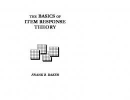
Figure 1. Relationship between probability predictions and Brier scores in events with binary outcomes.

Without any loss of generality, we set a = 0 and b = 1 in all our analyses. Figure 1 illustrates the relationship between probability predictions and Brier scores for binary cases (where 0 = outcome does not happen in blue, and 1 = outcome does happen in red). Brier scores measure the mean square difference between the predicted probability assigned to the possible outcomes and the actual outcome. Thus, lower Brier scores indicate better calibration of a set of predictions. In addition to motivating forecasters (Gneiting & Raftery, 2007), these scores provide a means of assessing relative accuracy as they reflect the “quality” or “goodness” of the probabilistic forecasts: The lower the mean Brier score is for a set of predictions, the better the predictions. Typically, scores do not take into account the characteristics of the events, or class of events, being forecast. Consider, for example a person predicting the results of games to be played between teams in a sports league (e.g., National Football League, National Basketball Association). A probability forecast, p, earns the same score if it refers to the outcome of a game between the best and worst teams in the league (a relatively easy prediction) or between two evenly matched ones (a more difficult prediction). Similarly, they give equal credit for assigning the same probabilities when predicting political races where one candidate runs unopposed (an event with almost no uncertainty) and in very close races (an event with much more uncertainty). This paper uses the Item Response Theory (IRT) framework (e.g., Embretson & Reise, 2000; Lord, 1980; van der Linden & Hambleton, 1996) to incorporate event characteristics and, in the process, provides a framework to identify superior forecasters. IRT is a stochastic model of test performance that was

1 1 + e−a j (θi −b j )

(2)

where θ i is the person’s ability, a j and b j are the item discrimination and item difficulty parameters, respectively. Pj (θ i ) is the model’s predicted probability that a person with ability θ i will respond correctly to item j with parameters a j and bj . From this point on, we will abandon the test theory terminology and embrace the corresponding forecasting terms. We will refer to expertise, instead of ability, and events, instead of items. Extending the IRT approach to the assessment of probabilistic forecasting accuracy could bridge the measurement gap between expertise and features of the target events (such as their discrimination and difficulty) by putting them on the same scale and modeling them simultaneously. The joint estimation of person and event parameters facilitates interpretation and comparison between forecasters. The conventional estimates of a forecaster’s expertise (e.g., his or her mean Brier score, based on all events forecast) are content dependent, so people may be assigned higher or lower “expertise” scores as a function of the events they choose to forecast. This is a serious shortcoming because (a) typically judges do not forecast all the events and (b) their choices of which events to forecast are not random. In fact, one can safely assume that they select questions strategically: Judges are more likely to make forecasts about events in domains where they believe (or are expected to) have expertise or events they perceive to be “easy” and highly predictable, so their Brier scores are likely to be affected by this self-selection that, typically, leads to overestimation of one’s expertise. Thus, all comparisons among people who forecast distinct sets of events are of questionable quality. A remedy to this problem is to compare directly the forecasting expertise based only on the forecasts to the common subset of events forecast by all. But this approach can also run into problems. As the number of forecasters increases, comparisons may be based on smaller subsets of events answered by all and become less reliable and informative. As an example, consider financial analysts who make predictions regarding future earnings of companies that are traded on the market. They tend to specialize in various areas, so it is practically impossible to compare the expertise of an analyst that focuses on the automobile industry and another that specialize in the telecommunication area, since there is no overlap between their two areas. Any difference between their Brier scores could be a reflection of how predicable one


yi j = b0j + (b1j − b0j )e−b2 ti j + λ j θ i + ei j

(3)

where t i j is the time at which individual i forecast item j (measured as days until the ground truth of the event is determined), b0j reflects item j’s easiness as days to item expiration goes to infinity, b1j reflects item j’s easiness at the time the item resolves (i.e., the item’s “irreducible uncertainty”), and b2 the describes change in item easiness over time. The underlying latent individual trait in Merkle et al.’s (2016) IRT model, θ i , measures expertise, but it is not linked with a proper scoring rule. When using a model to analyze responses, it is always beneficial and desirable to have the model reflect the respondents’ knowledge about the evaluation criterion in the testing environment. In the absence of such a match, one can question the validity of the scores obtained, as it is not clear that they measure the target construct. A good analogy is a multiple-choice test that is scored with a penalty for incorrect answers without informing the test takers of the penalty (Budescu & Bar-Hillel, 1993). In this paper we propose a new model that is based on the same scoring rule that is communicated to forecasters. More generally, we describe an IRT framework in which one can incorporate any proper scoring rule into the model, and we show how to use weights based on event features in the proper scoring rules. This leads to a model-based method for evaluating forecasters via proper scoring rules, allowing us to account for additional factors that the regular proper scoring rules rarely consider.

25000 5000 0

0

5000

15000

Frequency

25000

35000

Rounded distribution

35000

Empirical distribution

Frequency

industry is, compared to the other, and not necessarily of the analysts’ expertise and forecasting ability. An IRT model can solve this problem. Assuming forecasters are sampled from a population with some distribution of expertise, a key property of IRT models is invariance of parameters (Hambleton & Jones, 1993): (1) parameters that characterize an individual forecaster are independent of the particular events from which they are estimated; (2) parameters that characterize an event are independent of the distribution of the abilities of the individuals who forecast them (Hambleton, Swaminathan & Rogers, 1991). In other words, the estimated expertise parameters allow meaningful comparisons of all the judges from the same population as long as the events require the same latent expertise (i.e., a unidimensional assumption). Most IRT models in the psychometric literature are designed to handle dichotomous or polytomous responses and cannot be used to analyze probability judgments, which, at least in principle, are continuous. One recent exception is the model by Merkle, Steyvvers, Mellers and Tetlock (2016). They posit a variant of a traditional one-factor model, and assume that an individual i’s observed probit-transformed forecast yi j on event j is a function of the forecaster’s expertise θ i :

92

15000


0.0

0.4

0.8

forecasts

0.0

0.4

0.8

rounded forecasts

Figure 2. Distributions of the original probability forecasts and their rounded values

2 IRT Forecasting Model Consider a forecasting event j with K possible responses that is scored by a given proper scoring rule. Each response is assumed to follow a multinomial distribution with a probability of each possible response specified in equation (4, below). In most cases, each possible response links to one possible score, so an event with K possible responses, has K possible scores. Each possible score is denoted as s k where k = (1, . . . , K ) and s k ∈ [0, 1], with 0 being the best and 1 being the worst. The model’s predicted probability that the i’th (i = 1, . . . , N ) forecaster receives a score si j = s k ′ based on a proper scoring rule on the j’th ( j = 1, . . . , M) event conditioning on his/her expertise θ i is denoted as p(si j = s k ′ |θ i ). Proper scores in the model should match the proper scoring rule that motivates and guides the forecasters. In this paper we focus on the Brier scoring rule. The model predicts the probability via the equation e a j (1−sk ′ )(θi −(b j +ρk ′ )) p(si j = s k ′ |θ i ) = PK a (1−s )(θ −(b +ρ )) j i j k k k=1 e

(4)

Here a j is the event’s discrimination parameter, b j is its difficulty parameter, defined as the event’s location on the expertise scale, and ρk is a parameter associated with the k’th (k = 1, . . . , K ) possible score. The parameter ρk is invariant across events and reflects the responses selected and their associated scores. The model requires forecasts to be binned. Choosing a large number of bins (K ) would complicate and slow down the estimation process, especially when the data are sparse (as is the case in our application, to be described in the next



93

Event Discrimination when β=−1 and ρ6=−0.6

0.4

0.6

0.8

α=0.5 α=1 α=2 α=3

0.0

0.2

Model predicted ProbabilityPij

0.2

0.4

0.6

0.8

β=−2 β=−1 β=0 β=2

0.0


1.0

1.0

Event Difficulty when α=3 and ρ6=−0.6

−2

−1

0

1

2

Expertise

Figure 3. Item characteristic curves (varying only event difficulty b).

section). Thus, it is more practical to estimate the model with smaller values of K and we choose to set K = 6. Figure 2 shows the distribution of the probability responses that we used (see details below) in the left panel, and the distribution of the binned probabilities in the right panel. Clearly, the distribution of binned probabilities preserves the shape of the empirical distribution, so it is reasonable to assume that it contains most of the information needed to estimate the model parameters accurately. It is reasonable to assume the model would work better with more, say K = 11, bins so our results are essentially a lower bound for the quality of the method. Some key features of the model are illustrated in Figures 3 through 5. The curves plot the relationship between expertise and the probability of giving a perfect prediction (that maps into a Brier score, s k ′ =6 = 0) to events of different difficulties b j , event discriminations a j and the scaling parameter ρk=6 of a perfect prediction. The blue curve that is replicated in all three figures represents a “baseline” event with b j = −1, a j = 3 and ρk=6 = −0.6. The values of the other five scaling parameter ρk=1,. . . 5 are fixed in all the curves and they are (−0.02, −0.62, −0.58, −0.51, −0.56). Figure 3 shows how the model captures event difficulty. The four curves have the same discrimination and the same level of ρk=6 , but differ in event difficulty (b j ). The top curves represent easier events, and the bottom curves represent harder ones. For harder events, the probability of making perfect predictions with a Brier score of 0 (s k ′ =6 = 0) is lower at all levels of expertise. The stacked positions of the four curves show that for any expertise level, the model

−2

−1

0

1

2

Expertise

Figure 4. Item characteristic curves (varying only event discrimination a).

predicts probability increases for easier events. Figure 4 illustrates discrimination – the degree to which an event differentiates among levels of expertise. The four curves have the same difficulty level and the same values of ρk=6 , but differ in discrimination, which drives their steepness. The top curves represent the most discriminating events: they are steeper than the other two, so the probability of being correct changes rapidly with increases in expertise. Finally, Figure 5 shows the scaling parameter, ρk=6 . The model treats the probability forecasts as a discrete variable: with K possible probability forecast responses, there are K possible scores. The scaling parameter is necessary to link the score to the model. In our model, each event gets its own slope and own “location” parameters, but the differences among scores around that location are constrained to be equal across event. In other words, the values of ρk are fixed across all the items. Curves in Figure 5 have the same level of discrimination and difficulty, but differ with respect to ρk=6 . The pattern is similar to that in Figure 3, indicating that ρk=6 serves a similar function as event difficulty, with the difference being that the event difficulty parameter varies from event to event, while ρk=6 is fixed across all the events.

3 The relationship with Bock’s generalized nominal model Bock’s (1972) generalized nominal response model is an unordered polytomous response IRT model. The model states that the probability of selecting the h’th category response in



0.2

0.4

0.6

0.8

ρ6=−1 ρ6=−0.6 ρ6=−0.3 ρ6=−0.1

0.0


1.0

The Scaling Parameter of the Brier Score being 0 when β=−1 and α=3

−2

−1

0

1

2

Expertise

Figure 5. Item characteristic curves (varying only the scaling parameter ρ.

an item with m mutually exclusive response categories is: e ah (θ−bh ) p(h) (θ) = PK ah (θ−bh ) h=0 e

(5)

where ah and bh are the discrimination parameter and the difficulty parameter for the category h of the item. Our model (Equation 6) is a special case of the Bock’s model (Equation 7). The values of a j (1 − s k ′ ) and (b j + ρk ′ ) can be re-expressed as ak ′ and bk ′ and we can rewrite Equation (6) accordingly: e ak ′ (θi −bk ′ ) p(s k ′ |θ i ) = PK a k (θi −b k ) k=1 e

(6)

4 Parameter Estimation According to Fisher (1922, p. 310), a statistic is sufficient if “no other statistic that can be calculated from the same sample provides any additional information as to the value of the parameter.” The sufficient estimate of the judges’ expertise in our model is a monotonic transformation of the operational scoring rule. More specifically, in the current implementation (Equation 6), θ i is a weighted sum of eventspecific Brier scores for forecaster i across all events he/she forecasted (see derivation in Appendix A). The intuition is straightforward: each event-specific Brier score is weighted by the event’s level of discrimination, so that the more (less) discriminating an event is, the more we over (under) weigh it in estimating the judge’s expertise. Thus, our main prediction is that expertise estimates from the

94

model will be a more valid measure of the judges’ underlying forecasting expertise than the raw individual proper scores that weight all events equally. We take a Bayesian approach (see, e.g., Gelman, Carlin, Stern & Rubin, 1995) for the estimation of model parameters. This requires specification of prior distributions for all its parameters. The prior distribution for expertise parameters, θ i , was a standard normal distribution (zero mean and unit variance). For b j and ρk , we used vague normal distribution priors with a mean of 0 and standard deviations of 5. We rely on vague priors because we don’t have much prior information about the distributions of the event and the expertise parameters. We prefer to let the observed data (forecasts) find the distributions iteratively. We assume that the event discrimination parameter, a j , has a positively-truncated normal prior (Fox, 2010). Fixing this parameter to be positive makes the IRT model identifiable with respect to the location and scale of the latent expertise parameter. To summarize, the model parameters’ priors follow the Gaussian distributions with the means and variances shown below: θ i ∼ N (0, 1) a j ∼ N (0, 25) ∈ [0, +∞) b j ∼ N (0, 25) ρk ∼ N (0, 25).

(7)

We used the Just Another Gibbs Sampler (JAGS) program (Plummer, 2003) to sample posterior distribution in equation (5). JAGS is a program for analysis of Bayesian hierarchical models using Markov Chain Monte Carlo (MCMC) simulation. It produces samples from the joint posterior distribution. To check the convergence of the Markov chain to the stationary distribution1, we used two criteria: (1) Traceplots that show the value of draws of the parameter against the iteration number and allow us to see how the chain is moving around the parameter space; (2) A numerical convergence measure (Gelman & Rubin 1992) based on the idea that chains with different starting points in the parameter space converge at the point where the variance of the sampled parameter values between chains approximates the variance of the sampled parameter values within chains. A role of thumb states that the MCMC algorithm converges when the Gellman – Rubin measure is less than 1.1 or 1.2 for all parameters of the model (Gelman & Rubin 1992).

5 Implementing the model We illustrate the model by using the geopolitical forecasts collected by the Good Judgment Project (GJP) between 1The stationary distribution is the limiting distribution of the location of a random walk as the number of steps taken approaches infinity. In other words, a stationary distribution is such a distribution π that regardless of the initial distribution of π (0) , the distribution over states converges to π as the number of steps goes to infinity and is independent of π (0) .



95

Event−level correlations 1.0

Observed vs. Expected Response Frequencies

0.8 0.2

0.4

20000

−0.2

0.0

5000 10000

Frequencies

0.6

30000

Observed Frquencies Expected Frequencies

0.0

0.2

0.4

0.6

0.8

1.0

Responses

Figure 7. Boxplot of the event-level correlations between the observed and the expected response frequencies.

Figure 6. Observed and expected response frequencies at the global level.

September 2011 and July 2014 (Mellers et al. 2014; Mellers, Stone, Murray, Minster, Rohrbaugh, Bishop, Chen, Baker, Hou, Horowitz, Ungar and Tetlock, 2015; Tetlock, Mellers, Rohrbaugh and Chen, 2014). GJP recruited forecasters via various channels. Participation in the forecasting tournament required at least a bachelor’s degree and completion of a 2hour long battery of psychological and political knowledge tests. Participants were informed that the quality of their forecasts would be assessed using a Brier score (Brier, 1950) after the scoring was explained to them, and their goal was to minimize their average Brier score (across all events they chose to forecast). Mellers et al. (2014) provide further details about data collection. A unique feature of this project is that participants could choose which events to forecast. The average number of events forecasters predicted every year during the first three years of the tournament2 was 55. Overall there were approximately 458,000 forecasts from over 4,300 forecasters and over 300 forecasting events. The data set is very sparse, with almost 66% “missing” forecasts. We began by fitting the IRT forecasting model with the Brier scoring rule to a reduced, but dense, subset of the full GJP data set to avoid potential complications associated with missing data. This data set, created and used by Merkle et al. (2016), includes responses from 241 judges to 157 binary forecasting events). It contains responses of the most active and committed judges who made forecasts on nearly all the 2Year 4 data were not included in the calculation of mean average number of items predicted by the forecasters because data collection was ongoing at the time of the analysis.

events. Each judge forecast at least 127 events and each event had predictions from at least 69 judges. The mean number of events forecast by a judge was 144 and the mean number of forecasts per event was 221, and the data set included 88,540 observations.3 The percentage of missing data in this data subset was only 8%. They were treated as missing at random and were not entered into the likelihood function. The probabilistic forecasts were rounded to 6 equally spaced values (0.0, 0.2, 0.4, 0.6, 0.8 and 1.0) as shown in Figure 2. Convergence analyses show that the MCMC algorithm reached the stationary distributions, and Gelman & Rubin’s (1992) measures for all of the model’s parameters were between 1 and 1.5.4 Importantly, Gelman & Rubin’s (1992) measures for the estimated expertise parameters were all less than 1.2. The trace plots of the parameter estimates show that the chains mixed well. The trajectories of the chains are consistent over iterations and the corresponding posterior distributions look approximately normal. Model Checking. We compared the observed and expected response frequencies at the global level and the event level. The observed response frequencies are, simply, the counts of each of the 6 possible probability responses. The model calculates the probability of each of the 6 possible responses (0, 0.2, 0.4, 0.6, 0.8 and 1) for each unique combination of an event and a forecaster. The expected frequencies are 3Forecasters were allowed to give multiple predictions to the same item, and the response data set includes all the predictions made by a forecaster on an item and they were considered to be multiple independent observations for the same combination of judge and item. 4There is no guarantee of convergence of the MCMC algorithm in this (or any other) case, but that we are only using posterior means, rather than details of the exact posterior distribution, so the possible lack of convergence may not be a serious concern.

0

Table 1. Joint distribution of resolution type and goodness of fit in 157 events

Non statusquo

NC

Total

cor(observed, expected) ≥ 0.7 cor(observed, expected) < 0.7

113

19

3

135

7

13

2

22

Total

120

32

5

157

2

4

6

8

10

Item Brier score

0.39

−0.63 10

Statusquo

96


0.2 0.4 0.6 0.8 1.0


8

Item discrimination

Not Classified (NC) refers to events that cannot be classified as status-quo or not.

5Different items refer to various time horizons: In some cases the true outcome is revealed in a matter of a few weeks and in others only after many months. 6The items forecast are from different domains, including diplomatic relationship, leader entry/exit, international security/conflict, business 7Status-quo items ask about maintaining the existing social structure and/or values. For example, an item (“Before 1 March 2014, will Gazprom announce that it has unilaterally reduced natural-gas exports to Ukraine?”) contained an artificial deadline of March 1. The item resolved as the status quo, namely “no change” in the exports by the deadline. 8The mean estimate of θi being 0.04 and the mean estimate of ρk being

−10

the sums of the model predicted probabilities for each of the 6 possible responses aggregated across all events and forecasters. Figure 6 plots the observed and predicted response frequencies for each of the 6 possible responses across all events and respondents. The correlation between expected and observed values is 0.97. Figure 7 shows the distribution of the correlations between the expected and observed values at the event level (i.e., 157 correlations). One hundred and twenty of the 157 events (76.4%) have correlations above 0.9 and 15 of them (9.6%) have correlations between 0.7 and 0.9. Only 22 events (14%) of the correlations between observed and the expected frequencies are below 0.7. There is no obvious commonality to these events in terms of duration5 or domain6 but their estimated discrimination parameters are lower than the others (mean of 0.3 and a standard deviation of 0.27), suggesting that they don’t discriminate among levels of expertise. Interestingly, these are disproportionately events that resolved as change from the “status quo”, as shown in 7 Table 1.7 The odds ratio in the table is 113 19 / 13 = 11, and the Bayes factor in favor of the alternative that the variables are not independent is 8,938, which projects strong evidence against the null hypothesis. Results indicate that the model fits the forecasts for the status quo event better than the nonstatus quo events. In other words, it is harder to predict change than constancy. Parameter estimates. The events in this subset were relatively “easy”8 with only 15 out of 157 (9.5%) events hav-

−5

0

5

Item difficulty

10

0

2

4

6

0.17

0.2 0.4 0.6 0.8 1.0

−10

−5

0

5

10

Figure 8. The scatterplot matrix of the event Brier scores and the event parameter estimates.

ing positive b j estimates. The mean b j estimate was –1.37 (SD=2.70) and single event estimates ranged from –9.27 to 13.89. The mean discrimination, a j , was 2.29, and estimates ranged from 0.04 to 10.43. The mean estimated expertise, θ i , was 0.04 (SD = 0.96) with estimates ranging from –1.71 to 3.29. The estimated values of ρk (k = 1, . . . 6) were –0.04, –0.90, –0.86, –0.79, –0.84 and –0.88 for the score categories. The first value is distinctly different from the other five ρk (k = 2, . . . , 6).9 Relationship between Brier scores and the model parameter estimates. Figure 8 shows the scatter plot matrix (SPLOM) of the two event-level parameters and the events’ mean Brier scores. The diagonal of the SPLOM shows histograms of the three variables, the upper triangular panel shows the correlations between row and column variables, and the lower triangular panel shows the scatter plots. We observe a negative curvilinear relationship between the discrimination parameter a j and the Brier scores, indicating that events with higher mean Brier scores tend not to discriminate well among forecasters varying in expertise. Most of the b j -0.72 suggest that an item with a negative b j is relatively easy for a typical forecaster. 9The parameter ρ1 corresponds to the first response category (0), which has a Brier score of 1, so the numerator of the model’s predicted probability for s1 = 1 is 1 for all the expertise levels. That is, the model cannot use the information from the response data to estimate the ρ1 and the value is set to be the initial value plus some random noise from the prior distribution of ρk . On the other hand, if we were to exclude the component (1 − sk ), the model cannot be identified without a restriction on the ρk (for example, fixing ρ1 = 0). Therefore, the fact that the estimate of ρ1 is very close to 0 can be considered to approximate a constraint necessary for model identification.


0

1

2

3 3

−2 −1


Table 2. Polynomial and linear regressions of the expertise estimates as a function of the mean Brier scores.

2

Expertise_IRTForecasting

97

0.8

−2 −1

0.6 0.4 0.2 2

3

0.2

0.4

0.6

0.8

Figure 9. Scatter plot matrix of the IRT forecasting modelbased expertise estimates, Merkle et al.’s (2016) expertise estimates and the Brier scores.

2 1 −1

−1 −2

0

Regular forecasters’ expertise estimates

−2

estimates cluster around 0, with Brier scores ranging from 0 to 0.5. Among the events with Brier scores above 0.5, there is a positive relationship between Brier scores and difficulty parameters. The correlation between the discrimination and the difficulty parameters is low (.17), as they reflect different features of the events. We regressed the events’ mean Brier scores on the two parameters – discrimination and difficulty – and their squared values. The fit is satisfactory (R2 = 0.78; F (4, 152) = 131.6, p < .001), and all four predictors were significant. Figure 9 shows a SPLOM of the model’s expertise estimates, the mean Brier scores and the expertise estimates from Merkle et al.’s (2016) model of the 241 judges. We observe a negative curvilinear relationship between the model’s expertise estimates and the mean Brier scores. Judges with high expertise estimates had lower Brier scores. Table 2 shows results of linear and polynomial regressions predicting the expertise estimates. In the linear regression, the mean Brier score was the sole predictor, and the polynomial regression also included the squared mean Brier score. The R2 values for the linear and polynomial regressions are 0.72 and 0.84, respectively, indicating that the nonlinear component increases the fit significantly (by 12%). This non-linearity reflects the fact that the model uses different weights for different events as a function of the discrimination parameters to estimate expertise, a unique feature of the IRT-based expertise estimates. The relationship between Merkle et al.’s (2016) expertise estimates and mean Brier scores is also curvilinear, but the non-linearity is not as strong as that found

3

4

Super forecasters’ expertise estimates 4

1

Linear Regression of Model’s Expertise Estimate (n=241) Intercept 2.50 0.11 23.77