performance of IP networks by selecting proper positive definite matrices Q and ... traffic have drifted the network monitoring parameter outside its specified.
Self-tuning Optimal PI Rate Controller for End-to-End Congestion With LQR Approach Yang Hong and Oliver W.W. Yang 1
CCNR Lab, SITE, University of Ottawa, Ottawa, Ontario, Canada K1N 6N5 {yhong, yang}@site.uottawa.ca
Abstract. This paper presents a self-tuning optimal PI (Proportional-Integral) rate controller for end-to-end congestion in the IP-based Internet. We employ LQR (Linear Quadratic Regulator) approach from modern control theory in the optimal controller design that would allow the user to achieve good transient performance of IP networks by selecting proper positive definite matrices Q and R. Self-tuning PI rate controller self-tunes only when the changes in network traffic have drifted the network monitoring parameter outside its specified interval. The PI rate controller is located in each router and can calculate a desirable advertised source window size (i.e. source sending rate) based on the instantaneous queue length of the buffer. Our OPNET simulations demonstrate that our network traffic control algorithm can provide the network with a good transient behavior in AQM and flow throughput. Keywords: Rate-Based Control, Active Queue Management, Best-Effort Traffic, LQR Approach, Streaming Media Traffic.
1 Introduction Congestion control has been a critical factor in the robustness of the Internet [1] and its photonic infrastructure e.g., [2]. As a dominant end-to-end congestion control algorithm, TCP (Transmission Control Protocol) is widely implemented in current IP (Internet Protocol) networks [1]. In TCP/IP networks, the router applies AQM (Active Queue Management) algorithm (e.g., RED [3], PI-RED [4, 5] etc.) to implicitly inform the source the network congestion by dropping the packets. In the mean time, the source uses the AIMD (Additive Increase and Multiplicative Decrease) algorithm [6] to adjust its window size to prevent the congestion. They are all window-based control. The AIMD algorithm is very effective in the conventional IP networks where the propagation delays are short compared to the source sending rates. However, under the network environment with the long round trip delay and dynamically changing available bandwidth (e.g., the edge switches of the Agile All-Photonic Networks [2]), the AIMD control with AQM often yields severe fluctuations in the source sending rates and oscillation of queuing sizes in the routers [7, 8]. Such behavior greatly degrades the network performance and makes the AIMD control unsuitable for streaming media transmission [9, 10]. L. Mason, T. Drwiega, and J. Yan (Eds.): ITC 2007, LNCS 4516, pp. 829–840, 2007. © Springer-Verlag Berlin Heidelberg 2007
830
Y. Hong and O.W.W. Yang
Many attempts have been made to achieve a high QoS (Quality of Service) for streaming media transmission in the Internet. One of the challenges in designing congestion controller is to support streaming media traffic consisting of a variety of traffic classes with a different quality of service requirement. Rate-based control allows the sources to adjust their sending rates to support best-effort service traffic and makes the optimum use of network resources. Most of rate-based control schemes were originally used for high-speed ATM networks, e.g., [11, 12]. Some rate-based control methods have been proposed recently for the AQM router to support best effort service traffic (e.g., audio and video stream) in the IP networks. For example, the TFRC (TCP Friendly Rate Control) scheme proposed an equation in the source to calculate the source sending rate for unicast traffic based on the packet loss event [10, 13]. The VCP (Variable-Structure Congestion Control) Protocol [14] employed an improved AIMD scheme in the sources by using the existing two ECN bits for network congestion feedback, but the fluctuations of the source sending rates still remain. A rate-based control scheme was proposed for transparently augmenting the end-to-end performance by controlling the source sending rate in [15]. A two-state adaptive rate control mechanism was proposed for streaming media [9]. A rate-based window control method was presented in co-operation with the RED scheme to control best-effort traffic in an environment with packet loss and varying round-trip delays [16]. However, most of these rate-based feedback control algorithms for IP networks are heuristics that lack a control theoretical analysis, so they cannot always guarantee the closed-loop stability in different traffic conditions. The XCP (Explicit Congestion Control) protocol [7] did apply the simple control theoretical analysis to calculate the advertised source sending rates in the routers based on the spare network bandwidth and the queue length, but it cannot cancel the steady state error due to the estimation error of the link capacity [17]. Furthermore, the choices of the XCP parameters cannot guarantee its desirable network performance in different network environment [17, 18]. In summary, all these discussed rate-based algorithms did not consider the optimal solution for the network performance of AQM control system. The main contributions of this paper are: 1) Unlike all other papers that propose heuristic rate-based algorithms for the AQM control system (either applying frequency domain or time domain analysis from the classical control theory), we use instead the state space approach from the modern control theory to describe the network model for a typical AQM router in the IP-based Internet (shown in Fig. 2 later on). 2) We employ the LQR (Linear Quadratic Regulator) approach to obtain our optimal PI rate controller that can achieve good transient performance. We have derived for the first time Equations (24) and (25) to calculate the PI controller parameters, where PI controller is used to regulate the source sending rates. 3) Allowing our controller to self-tune the controller parameters upon the network traffic changes so that the closed-loop stability of rate-based AQM control is always guaranteed. To the best of our knowledge, no other papers on rate-based control algorithms applied the optimal control and adaptive control jointly in the controller design. We have verified all the claims above by OPNET simulations to show that our control scheme serves both guaranteed service traffic and best-effort service traffic well, while achieving maximum bandwidth utilization of the Internet.
Self-tuning Optimal PI Rate Controller for End-to-End Congestion With LQR Approach
831
2 Network Model We consider a data communication network consisting of a number of geographically distributed source/destination nodes. IP packets generated at a source node are delivered to their destination through a sequence of AQM routers in the Internet. The PI rate controller is located in the router and can calculate a desirable source window size (i.e. source sending rate λ'i (t ) ) based on the instantaneous queue length of the buffer in the router, and advertise it to the source through the IP packet and the ACK packet so that the source can regulate its current sending rate λi(t) to provide the besteffort service traffic. There is also an uncontrolled guaranteed service traffic flows (both local and from the upstream router) with input rate υ(t) into the router. τ b1
λ1 (t )
λ1' (t ) υ(t)
τ f1 • • •
λ N (t )
μ y (t )
τ fN τ bN
λ'N (t )
Fig. 1. System Model of the AQM Router
The AQM router under consideration accumulates multiple best-effort service traffic streams and one guaranteed service traffic stream, as shown in Fig. 1. There are N controlled source nodes that transmit the packets routed through the AQM router. The AQM router has a finite buffer space K to store the incoming packets and an output link to serve them at a constant data rate of μ. It is assumed that the service for the queue is FIFO (First-Input First-Output) and the best-effort service traffic and the guaranteed service traffic enter the same queue and share the common bandwidth of the output link. The guaranteed service traffic will not be influenced by the congestion situation of the router, i.e. their source sending rates are guaranteed. There are two kinds of time delays: (1) the varying forward time delay τfi from the controlled source node i to the router; which includes propagation delay, queuing delay and processing delay; (2) the varying feedback time delay τbi of both from the router to the controlled source node i via the destination, which also includes propagation delay, queuing delay and processing delay. We can let τi=τfi+τbi be the varying round trip time of the controlled source node i. From the AQM router model in Fig. 1, the change of the queue length in the buffer of the router is the sum of the input rates of both the N best-effort service traffic flows and the guaranteed service traffic flows minus the service rate. It can be written as
832
Y. Hong and O.W.W. Yang N
y� (t ) = ∑ λi (t − τfi ) + υ(t) − μ . i =1
(1)
3 Self-tuning Optimal PI Rate Controller Design We propose a self-tuning optimal PI rate controller that can achieve zero queue deviation in the router and prevent the Internet from congestion. Every controlled source node is allowed to send the packets into the network at its maximum allowed sending rate in order to utilize the spare bandwidth unused by the guarantee service traffic. Let y0 be the target buffer occupancy of the buffer in the AQM router. Let the parameters KP and KI be the proportional gain and integral gain of PI rate controller at the router, which are two important parameters in our controller design. Based on the instantaneous queue length y(t) of the buffer, the advertised sending rate λ'i (t ) for the controlled source node i can be obtained by the following PI rate control structure: λi' (t ) = λ' (t) = K Pe(t) + K I ∫0t e(τ )dτ = K P (y0 − y(t)) + K I ∫0t (y0 − y (τ ))dτ .
(2)
where e(t) indicates the difference between y(t) and y0. It can be seen from the control structure in Equation (2) that the advertised source rate λ'i (t ) is calculated based on the instantaneous queue length of the buffer. Since the advertised source sending rate λ'i (t ) becomes the source rate λi(t) after a feedback time delay of τbi, we can write λi (t ) = λi' (t − τ bi ) .
(3)
By substituting Eq. (3) into Eq. (1), we can capture the dynamics of the router as N
N
i =1
i =1
y� (t ) = ∑ λi' (t − τ bi - τfi ) + υ(t) − μ = ∑ λ'i (t − τi ) + υ(t) − μ .
(4)
To simplify the controller design, we can approximate the standardized round trip time by the average value τ of τi, i.e. τ = ∑iN=1τ i N . Such control plant approximation has been widely adopted in industrial process control system design, e.g., [19-23], which has found its application in network traffic control recently, e.g., [4, 7]. The validity of this approximation has been verified by our performance evaluation later on. Therefore, under this approximation, we can update Equation (4) as y� (t ) = Nλ' (t − τ ) + υ(t) − μ .
(5)
Note that we only design our optimal controller based on the plant approximation. We implement our control algorithm in the real network environment by OPNET simulations without any plant approximation in this paper. 3.1 Controller Design with LQR Approach To design our optimal PI rate controller via LQR approach [19], we need to translate the AQM control system described by time domain method in Fig. 1 into a state
Self-tuning Optimal PI Rate Controller for End-to-End Congestion With LQR Approach
833
feedback AQM control system. We will summarize the key steps for the optimal controller design in the following due to space limitation. To start, let x=[x1 x2]T such that x1 = ∫0t e(τ )dτ and x2=e(t) represent/capture the queue deviation. Also let u = λ' (t ) such that u = Kx = [ K I
K P ][ x1
x2 ]T .
(6)
Equations (2) and (5) can now be represented by the state space equations as follows: ⎡0 1 ⎤ ⎡ 0 ⎤ ⎡0⎤ ⎡0 ⎤ x� = ⎢ ⎥x + ⎢ ⎥u (t − τ ) + ⎢ ⎥υ + ⎢ ⎥ μ . ⎣0 0 ⎦ ⎣− N ⎦ ⎣− 1⎦ ⎣1 ⎦
(7)
Equation (7) can now be represented by Fig. 2. Our LQR problem is to find the optimal control u(t) such that J is minimized when ∞
J = ∫0 ( x T (t )Qx(t ) + u T (t ) Ru (t ))dt .
(8)
where Q and R are given positive definite matrices with proper dimensions (u(t)=0 when t0) [19, 24].
∫ y0 +
x1
KI
e(t) x2
-
KP
+
u
τ
N
υ (t ) + +
+
∫
y(t)
μ
Fig. 2. State Feedback AQM Control System
Considering that μ and υ are uncontrolled variables, we can now decompose the control system in Equation (7) into two different time periods [19, 20]: x� (t ) = Ax(t ) + Bu (t − τ ) = Ax(t ) when 0≤t