landmark-based shape correspondence used for statistical shape analy- sis. .... Eq. (1), and (C5) comparing the derived PDM N(¯v, D) to the ground truth.
A New Benchmark for Shape Correspondence Evaluation Brent C. Munsell, Pahal Dalal, and Song Wang Department of Computer Science and Engineering University of South Carolina, Columbia, SC 29208, USA {munsell,dalalpk,songwang}@engr.sc.edu
Abstract. This paper introduces a new benchmark study of evaluating landmark-based shape correspondence used for statistical shape analysis. Different from previous shape-correspondence evaluation methods, the proposed benchmark first generates a large set of synthetic shape instances by randomly sampling a specified ground-truth statistical shape model. We then run the test shape-correspondence algorithms on these synthetic shape instances to construct a new statistical shape model. We finally introduce a new measure to describe the difference between this newly constructed statistical shape model and the ground truth. This new measure is then used to evaluate the performance of the test shapecorrespondence algorithm. By introducing the ground-truth statistical shape model, we believe the proposed benchmark allows for a more objective evaluation of the shape correspondence than those that do not specify any ground truth.
1
Introduction
Statistical shape models have been applied to address many important applications in medical image analysis, such as image segmentation for desirable anatomic structures [1,2] and accurately locating the subtle difference of the corpus-callosum shapes between the schizophrenia patients and normal controls [3]. Accurate and efficient shape-correspondence algorithms [4,5] to identify corresponded landmarks are essential to the accuracy of the constructed statistical shape models. However, how to objectively evaluate the results produced by these shape-correspondence algorithms is still a very difficult problem. One major reason is the unavailability of a ground-truth shape correspondence: given a set of real shape instances, say the kidney contours from a group of people, even the landmark points identified by different experts may show substantial difference from each other [6]. To address this problem, Davies and Styner [6] introduce three general measures to describe the compactness, specificity, and generality of the statistical shape model constructed from a shape-correspondence result and suggest the use of these three measures for evaluating shape-correspondence performance. However, without introducing the ground truth, these three measures may not be reliable in some cases [7]. For example, according to these measures, we prefer N. Ayache, S. Ourselin, A. Maeder (Eds.): MICCAI 2007, Part I, LNCS 4791, pp. 507–514, 2007. c Springer-Verlag Berlin Heidelberg 2007 �
508
B.C. Munsell, P. Dalal and S. Wang
a shape correspondence that leads to a statistical shape model with high compactness (or smaller shape variation space), which may not be true for certain structures. In this paper, we present a new benchmark study with ground truth to more objectively evaluate the shape correspondence for statistical shape analysis. Specifically, the statistical shape analysis chosen for this paper is the widely used point distribution model (PDM) [1]. For simplicity, this paper focuses on the 2D case, where a point distribution model (PDM) is a 2m-dimensional Gaussian distribution with m being the number of landmarks identified from each shape instance. In this benchmark, we start with a ground-truth PDM by specifying a 2m-dimensional mean-shape vector and a 2m × 2m covariance matrix. We then randomly sample this PDM to generate a set of synthetic continuous shape instances. A test shape-correspondence algorithm is then applied to correspond these shape instances by identifying a new set of landmarks. Finally we construct a new PDM from the corresponded landmarks and compare it with the ground truth PDM to evaluate the accuracy of the shape correspondence.
2
Problem Description
Given n sample shape instances (or continuous shape contours in the 2D case) Si , i = 1, 2, . . . , n, shape correspondence aims to identify corresponded landmarks from them. More specifically, after shape correspondence we obtain n corresponded landmark sets Vˆi , i = 1, 2, . . . , n from Si , i = 1, 2, . . . , n, respectively. ˆ i2 , . . . , v ˆ im } are m landmarks identified from shape contour Si Here Vˆi = {ˆ vi1 , v ˆ ij = (ˆ and v xij , yˆij ) is the jth landmark identified along Si . Landmark correˆij , i = 1, 2, . . . , n, i.e., the jth landmark in each shape spondence means that v contour, are corresponded, for any j = 1, 2, . . . , m. In practice, structural shape is usually assumed to be invariant to the transformations of any (uniform) scaling, rotation, and translations. Therefore, shape normalization is applied to Vˆi , i = 1, 2, . . . , n to remove such transformations among the given n shape contours. Denote the resulting landmark sets to be Vi = {vi1 , vi2 , . . . , vim }, i = 1, 2, . . . , n, in which the absolute coordinates of the corresponded landmarks, e.g., vij = (xij , yij ), i = 1, 2, . . . , n are directly comparable. Finally, we calculate the statistical shape model by fitting the normalized landmarks sets Vi = {vi1 , vi2 , . . . , vim }, i = 1, 2, . . . , n to a multivariate Gaussian distribution. Specifically, we columnize m landmarks in Vi into a 2m-dimensional vector vi = (xi1 , yi1 , xi2 , yi2 , . . . , xim , yim )T and call it a (landmark-based) shape ¯ and the vector of the shape contour Vˆi . This way, the mean shape vector v covariance matrix D can be calculated by 1� vi , n i=1 n
¯= v
1 � ¯ )(vi − v ¯ )T . (vi − v n − 1 i=1 n
D=
(1)
The Gaussian distribution N (¯ v, D) is the resulting PDM that attempts to model the deformable or probablistic shape space of the considered structure.
A New Benchmark for Shape Correspondence Evaluation
509
The accuracy of the PDM is largely dependent on the performance of shape correspondence, i.e., the accuracy in identifying the corresponded landmarks Vˆi , i = 1, 2, . . . , n. However, the performance of shape correspondence is not well defined because in practice, a ground-truth shape correspondence is usually not available and the landmarks manually labeled by different experts may be quite different from each other [6].
3
Proposed Method
The proposed benchmark starts from a specified ground-truth PDM, from which we can randomly generate a set of synthetic shape contours. A shapecorrespondence algorithm should be able to identify corresponded landmarks from these shape contours and leads to a PDM that well describes the shape space defined by the ground-truth PDM. As shown in Fig. 1, the proposed benchmark consists of the following five components: (C1) specifying a PDM N (¯ vt , Dt ) as the ground truth, (C2) using this PDM to randomly generate a set of shape contours S1 , S2 , . . . , Sn , (C3) running the test shape-correspondence algorithm on these shape contours to identify a set of corresponded landmark sets, (C4) deriving a PDM N (¯ v, D) from the identified landmark sets using Eq. (1), and (C5) comparing the derived PDM N (¯ v, D) to the ground truth PDM N (¯ vt , Dt ) and using their difference to measure the performance of the test shape-correspondence algorithm.
C1
C2
C3
C4
S1 T1−1
S2
Ground Truth
PDM N ( v t, Dt )
T2
Sn Tn
Execute the Test Shape−Correspondence Algorithm
T1
−1
T2
PDM N ( v , D)
T n−1
C5 Compare Two PDMs
Δb
Fig. 1. An illustration of the proposed shape-correspondence evaluation benchmark
We can see that, in essence, this benchmark evaluates the shape-correspondence algorithm’s capability to recover the underlying statistical shape model from a
510
B.C. Munsell, P. Dalal and S. Wang
set of sampled shape instances. This reflects the role of the shape correspondence in statistical shape modeling. In these five components, (C3) and (C4) are for PDM construction and have been discussed in detail in Section 2. The task of ¯ t and a covariance matrix Component (C1) is to specify a mean shape vector v t t D . Ideally, they can take any values only if D is positive definite. In practice, we can pick them to resemble some real structures as detailed in Section 4. In this section, we focus on developing algorithms for Components (C2) and (C5). 3.1
Generating Shape Instances
Given the ground-truth PDM N (¯ vt , Dt ) with k landmarks (k might be different from m, the number of landmarks identified by shape correspondence in Component (C3)), we can randomly generate as many sample shape vectors vit , i = 1, 2, . . . , n as possible. More specifically, with ptj and λtj , j = 1, 2, . . . , 2k being the eigenvectors and eigenvalues of Dt , we can generate shape instances in the form of ¯t + vt = v
2k �
btj ptj ,
(2)
j=1
where btj is independently and randomly sampled from the 1D Gaussian distribution N (0, λtj ), j = 1, 2, . . . , 2k. t t Each shape vector vit , i = 1, 2, . . . , n in fact defines k landmarks {vi1 , vi2 ,..., t vik }. By assuming that these k landmarks are sequentially sampled from a continuous shape contour, we can estimate this continuous contour Si� by landmark interpolation. For constructing a closed shape contour, we interpolate the port t and the first landmark vi1 . For constructing tion between the last landmark vik t t an open shape contour, we do not interpolate the portion between vik and vi1 . While we can use any interpolation technique to connect these landmarks into contours, we use the Catmull-Rom cubic spline in this paper. If the ground-truth landmarks are sufficiently dense to represent the underlying shape contour (this is usually required for shape correspondence [8]), we expect that different interpolation techniques do not introduce much difference in the resulting shape contour. For each synthetic shape contour Si� , we also apply a random affine transformation Ti , consisting of a random rotation, a random (uniform) scaling and a random translation. We define the resulting continuous contour to be the shape contour Si . We record the affine transformation Ti , i = 1, 2, . . . , n and then pass S1 , S2 , . . . , Sn (in fact, their control points) to the test shape-correspondence algorithm. Note that the recorded affine transformations Ti , i = 1, 2, . . . , n are not passed to the test shape-correspondence algorithm (Component (C3)). This way, we test the capability of the shape-correspondence algorithm to handle affine transformations among the different shape contours. If the test shapecorrespondence algorithm introduces further transformations, such as Procrustes analysis, in Component (C3), we record and undo these transformations before
A New Benchmark for Shape Correspondence Evaluation
511
outputting the shape-correspondence result. This ensures the corresponded landmarks identified by the test shape-correspondence algorithm are placed directly back onto the input shape contours S1 , S2 , . . . , Sn . Then in Component (C4), we directly apply the inverse transform Ti−1 , i = 1, 2, . . . , n, to the landmarks identified on Si . This guarantees the correct removal of the random affine transformation Ti before PDM construction in Component (C4). 3.2
Comparing a PDM Against the Ground Truth PDM
The goal of comparing the PDM N (¯ v, D) derived in Component (C4) against the ground-truth PDM N (¯ vt , Dt ) is to quantify the difference of the deformable shape spaces that are represented by these two PDMs. However, directly com¯ puting the �2 norms (or any other vector or matrix-based norms) between v ¯ t , or D and Dt can not achieve this goal. In fact, in these two PDMs, the and v number of landmarks identified from each shape contour can be different, i.e., ¯ ∈ R2m , v ¯ t ∈ R2k and m �= k, where m and k are the number of landmarks v along each shape contour in these two PDMs. The reason is that, when using different shape-correspondence algorithms, or the same shape-correspondence algorithm with different settings, we may get different number of corresponded landmarks along each shape contour. Therefore, in this paper we compare two PDMs in the continuous shape space instead of using the sampled landmarks. For example, we can estimate the con¯t tinuous mean shape contours S¯t and S¯ by interpolating the landmarks in v ¯ , respectively. In our experiments, we use the Catmull-Rom spline for this and v interpolation. After that, we measure the difference of two continuous shape contours using the widely used Jaccard’s coefficient, which is landmark independent. More specifically, the mean-shape difference is defined as ¯ ¯t ¯ S¯t ) = 1 − |R(S) ∩ R(S )| , Δ(S, ¯ ∪ R(S¯t )| |R(S)
(3)
where R(S) indicates the region enclosed by the contour S and |R| computes the area of the region R. If S is an open contour, we connect its two endpoints by a straight line to form a closed contour for calculating R(S) [8]. We can see that this difference measure takes value in the range of [0, 1] with 0 indicating that S¯ is exactly the same as S¯t . ¯ S¯t ) = 0 does not guarantee the shape spaces represented by the However, Δ(S, two PDMs are the same. To evaluate the difference between the two shape spaces, we use a random-simulation strategy: randomly generating a large set of N shape vectors from each PDM using Eq. (2), interpolating these landmarks defined by these shape vectors into continuous shape contours, and then measuring the similarity between these two sets of shape contours. We denote the N continuous c and the N shape contours generated from PDM N (¯ v, D) to be S1c , S2c , . . . , SN continuous shape contours generated from the ground-truth PDM N (¯ vt , Dt ) to t t t be S1 , S2 , . . . , SN . When N is sufficiently large, the difference between these two sets of continuous shape contours can well reflect the difference of the shape spaces underlying these two PDMs.
512
B.C. Munsell, P. Dalal and S. Wang
Given two continuous shape contours, we can measure their difference using Eq. (3). Therefore, the problem we need to solve is to measure the difference t N between shape-contour sets {Sic }N i=1 and {Sj }j=1 with a given difference measure between a pair of shape contours, i.e., Δ(Sic , Sjt ), i, j = 1, 2, . . . , N . In this paper, we suggest the use of the bipartite-matching algorithm to evaluate the difference between these two shape-contour sets. In the bipartite-matching algorithm, an optimal one-to-one matching is derived between two shape-contour sets so that the total matching cost, which is defined as the total difference between the matched shape contours, is minimal. Based on this, we define a difference measure between these two PDMs as �N c t i=1 Δ(Si , Sb(i) ) , (4) Δb � N t where Sic and Sb(i) are the matched pair of shape contours in the bipartite matching. In this difference measure, we introduce a normalization over N so that Δb takes values in the range of [0, 1]. Using the bipartite-matching algorithm, the measure Δb assesses not only whether the two shape spaces (defined by two PDMs) contain similar shape contours, but also whether a shape contour has the same or similar probability density in these two shape spaces.
4
Experiments
In this section, we use the proposed benchmark to evaluate five 2D shapecorrespondence algorithms: Richardson and Wang’s implementation of an algorithm that combines landmark sliding, insertion and deletion (SDI) [8], Thodberg’s implementation of the minimum description length algorithm (T-MDL) [9], Ericsson and Karlsson’s implementation of the MDL algorithm (E-MDL) [7], Ericsson and Karlsson’s implementation of the MDL algorithm with curvature distance minimization (E-MDL+CUR) [7], and Ericsson and Karlsson’s implementation of the reparameterisation algorithm by minimizing Euclidean distance (EUC) [7]. While, in principle, the ground truth PDM can be arbitrarily specified, we intentionally construct it to make it resemble some real anatomic structures. The basic idea is to collect real shape contours of a certain structure, apply any reasonable available shape-correspondence algorithm on them and then construct a PDM using Procrustes analysis and Eq. (1). In our experiment, this shape correspondence is achieved by manually labeling one corresponded landmark on each shape contour and then picking the others using a uniform sampling of the shape contour. For open shape contours, such as kidney and femur, we assume the endpoints are corresponded across all the shape contours and therefore manual labeling is not needed. We use these PDMs as ground truth for the proposed benchmark. Specifically, in our experiments we collect kidney, corpus callosum (callosum for short), and femur contours and construct three groundtruth PDMs, all with 64 landmarks.
A New Benchmark for Shape Correspondence Evaluation
513
From each ground-truth PDM, we randomly generate n = 800 sample shape contours that are passed to the shape-correspondence algorithm for testing. In the random simulation for Δb , we generate N = 2, 000 sample shape contours from both the ground-truth PDM and the PDM constructed from the shapecorrespondence result. In addition, in evaluating each shape-correspondence algorithm on each ground-truth PDM, 50 rounds of random simulations are conducted to analyze the stability of Δb . For all five test shape-correspondence algorithms, we set the expected number of corresponded landmarks to be 64 in Component (C3). For bipartite matching, we use the cost scaling push relabeling algorithm implemented by Goldberg and Kennedy [10] with a complex√ ity of O( V E log(CV ), with V and E being the number of vertices and edges and C being the maximum edge weight when scaled and rounded to integers. Callosum
Kidney
Femur
0.23
0.1
0.075
0.22
0.095
0.07
0.21 Truth
0.09
0.065
SDI
T−MDL
Δ
b
Δ
b
Δ
E−MDL+CUR
b
0.2
E−MDL 0.085
0.06
0.19
EUC 0.055
0.08 0.18
0.075
0.05
0.17
0.16 0
5
10
15
20
25
30
35
Number of Simulations
40
45
50
0
5
10
15
20
25
30
35
Number of Simulations
40
45
50
0.045
0
5
10
15
20
25
30
35
40
45
50
Number of Simulations
Fig. 2. Δb obtained from three ground-truth PDMs that resemble (a) kidney, (b) callosum, and (c) femur, respectively. The x-axis indicates the round of the random simulation. The curves with dimond show Δb between each ground-truth PDM and itself.
The evaluation results are shown in Fig. 2, from which we can see that the values of Δb do not significantly change over the 50 random simulations. It also shows that, in general, the performance of T-MDL is lower than the performance of SDI, E-MDL, E-MDL+CUR, and EUC on all three ground-truth PDMs. SDI has a similar performance to E-MDL, E-MDL+CUR, and EUC for the groundtruth PDM that resembles the kidney while has a lower performance than EMDL, E-MDL+CUR, and EUC for the ground-truth PDMs that resemble the callosum and femur. In general, the performance of E-MDL, E-MDL+CUR, and EUC are all similar to each other. Note that, different shape-correspondence algorithms may be more suitable for different ground-truth PDMs. Also note that, the choices of n and N depend on the variance of the ground-truth PDM: if the ground-truth PDM has large eigenvalues along many principal directions, we may need to choose larger values for n and N . In this paper, the groundtruth PDMs resemble several real structures with limited variance. In fact, the stability of the Δb value over 50 rounds of random simulations may indicate that N = 2, 000 is sufficiently large. In addition, if a shape-correspondence algorithm produces a Δb value that is close to the Δb value between the ground-truth PDM and itself, this may indicate that n = 800 is sufficiently large.
514
5
B.C. Munsell, P. Dalal and S. Wang
Conclusion
In this paper, we introduced a new benchmark for evaluating the landmark-based shape-correspondence algorithms. Different from previous evaluation methods, we started from a known ground-truth PDM and then evaluate shape correspondence by assessing whether the resulting PDM describes the shape space defined by the ground-truth PDM. We introduced a new measure to quantify this difference. We applied this benchmark to evaluate five available 2D shape correspondence algorithms.
Acknowledgements This work was funded by NSF-EIA-0312861 and AFOSR FA9550-07-1-0250.
References 1. Cootes, T., Taylor, C., Cooper, D., Graham, J.: Active shape models - their training and application. Computer Vision and Image Understanding 61(1), 38–59 (1995) 2. Leventon, M., Grimson, E., Faugeras, O.: Statistical shape influence in geodesic active contours. In: IEEE Conference on Computer Vision and Pattern Recognition, pp. 316–323 (2000) 3. Bookstein, F.: Landmark methods for forms without landmarks: Morphometrics of group differences in outline shape. Medical Image Analysis 1(3), 225–243 (1997) 4. Davies, R., Twining, C., Cootes, T., Waterton, J., Taylor, C.: A minimum description length approach to statistical shape modeling. IEEE Transactions on Medical Imaging 21(5), 525–537 (2002) 5. Wang, S., Kubota, T., Richardson, T.: Shape correspondence through landmark sliding. In: IEEE Conference on Computer Vision and Pattern Recognition, pp. I–143–150 (2004) 6. Styner, M., Rajamani, K., Nolte, L.P., Zsemlye, G., Szekely, G., Taylor, C., Davies, R.: Evaluation of 3D correspondence methods for model building. In: Information Processing in Medical Imaging Conference (2003) 7. Ericsson, A., Karlsson, J.: Geodesic ground truth correspondence measure for benchmarking. In: Swedish Symposium in Image Analysis (2006) 8. Richardson, T., Wang, S.: Nonrigid shape correspondence using landmark sliding, insertion and deletion. In: International Conference on Medical Image Computing and Computer Assisted Intervention, pp. II–435–442 (2005) 9. Thodberg, H.: Minimum description length shape and appearance models. In: Information Processing in Medical Imaging Conference, pp. 51–62 (2003) 10. Goldberg, A., Kennedy, R.: An efficient cost scaling algorithm for the assignment problem. Mathematic Programming 71, 153–178 (1995)