Dec 11, 2001 - Each base station covers a geographical range called a cell. ... The allocation of the users can be guided by the load balancing principle.
Load balancing in cellular networks using first policy iteration Johan van Leeuwaarden, Samuli Aalto, Jorma Virtamo Helsinki University of Technology Networking Laboratory P.O. Box 3000, FIN-02015 HUT Finland December 11, 2001 Abstract This paper discusses load balancing in cellular networks. We compare the performance of both static and dynamic allocation policies for a simple model of two base stations with overlapping cells. In particular, we investigate the performance of the policy obtained by the first step of the policy iteration algorithm (FPI policy). When starting with a static policy, the two base stations can be modeled independently as Erlang loss systems, for which we can easily determine the relative costs in each state. This makes the first step of the policy iteration algorithm of low complexity, and therefore applicable for large instances. The idea is to approximate the optimal policy with the FPI policy. Numerical experiments for small instances provide a deeper understanding of the FPI policy. As it turns out, the optimal static policy not necessarily leads to the best performance of the FPI policy. When choosing an appropriate static policy, we show that the FPI policy is extremely close to the optimal policy, and performs much better than the other considered policies. This strengthens our belief in the practical relevance of the FPI policy.
1 Introduction A wireless network consists of fixed base stations and mobile users who communicate with the base stations via wireless links. Each base station covers a geographical range called a cell. Neighboring cells overlap with each other, which ensures continuity when users move from one cell to another. The users require communication channels at the base stations, whereas each base station can serve the users within its geographical range. Users that find themselves in an overlapping area, can be routed to either one of the base stations. The users that are in a non-overlapping area have to be routed to the corresponding base station, and are in that sense dedicated. Blocking occurs when a base station has no free channel to allocate to a user. The way users are allocated over the base stations influences the blocking probability. The allocation of the users can be guided by the load balancing principle. This principle says to balance the workload over the base stations, or, more colloquially, divide the load as evenly as possible, aiming to optimize performance measures of the system. Since we consider base stations with finitely many channels, our primary objective in our analysis is to minimize the blocking probability. Based on the load balancing principle, we consider different allocation policies that define the way users are allocated over the base stations. An important element hereby is the available information, which can range from total knowledge about the system at any point in time, to only information about basic characteristics like arrival rates and service times. We consider both static and dynamic policies. Static policies operate under time independent characteristics of the system, whereas dynamic policies operate under time dependent information. 1
It is somehow obvious that the more information an allocation policy is based on, the better it can perform. However, since more information incurs more costs and is more technically demanding, it could be advantageous to have an allocation policy of low complexity, and thus requiring little information about the system’s state. Moreover, practical applications have prohibitively large state spaces, rendering the direct computation of optimal dynamic policies impossible. For those reasons, a simple static policy is oftentimes used in practice. An idea introduced by Ott and Krishnan [9] makes it possible to construct a dynamic policy using a onestep improvement of the policy iteration algorithm. Independence assumptions embodied by an initial static policy make this method of low computational complexity. Numerical experiments showed that this policy could be close to the optimal policy, although its performance is heavily influenced by the initial static policy used (see e.g [6]). Our aim in this paper is two-fold. We consider the simple model of two base stations with overlapping cells. First, using only moderate instance sizes, we compare and illuminate the performance of different allocation policies for this model. Second, we gain insight in the performance of the one-step improvement in relation with the chosen initial static policy. We show that a well-chosen initial static policy makes the policy resulting from the one-step improvement close to optimal, which justifies its relevance for real-life applications. The remainder of this paper is structured as follows. In section 2 we describe the basic model. In section 3 we consider two static routing policies: optimized random routing and round-robin. In section 4 we consider dynamic routing policies, like overflow routing, least loaded routing and policies determined by the policy iteration algorithm. In particular, we pay attention to the one-step improvement and compare its performance with both the static and the other dynamic allocation policies. In section 5 we discuss three open problems for this paper’s model.
2 Model description We consider the case of two base stations BS1 and BS2 with overlapping cells as shown in figure 1.a. Based on their geographical positions, we can distinguish three types of users. Two of them form dedicated streams, which means that the users of those streams are always routed to the same base station, whereas the third user type forms a flexible stream; users of that stream may be routed to either one of the base stations. Furthermore, we take the arrival processes to be Poisson processes of rates λ1 and λ2 for the dedicated streams and ν for the flexible stream, and the service times to be exponentially distributed with parameter µ for both base stations. Both base stations have finitely many channels equal to c1 and c2 respectively. We denote the number of users at each base station at time t by i1 (t) and i2 (t). Without loss of generality, we assume that λ1 ≥ λ2 and µ = 1. An alternative way of visualizing the system is shown by figure 1.b.
λ1 BS1
BS2
c1
c2
11 00 00 11
ν
1 0 0 1
λ2
(a)
µ BS1 c1 1 0 0 1
BS2 c2
µ
(b)
Figure 1: (a) Two base stations with overlapping cells. (b) Traffic allocation model with dedicated streams.
This leaves us to specify the allocation policy, which we denote by α, to be used for routing the users of the flexible stream to either one of the base stations. Once the allocation policy α is specified, all 2
characteristics are known to draw the flow diagram as depicted in figure 2. Figure 2.a shows all transitions that are independent of the allocation policy used, while figure 2.b shows the rates of the flexible stream that do depend on α. The set of all possible states S is given by S = {(i1 , i2 )|i1 ≤ c1 , i2 ≤ c2 , (i1 , i2 ) ∈ Z2 }. i2
i2
c2
c2
λ2
ν λ1
i1
ν ν
λ2
i2
λ1
i1 i2
ν λ2
ν routed to BS 2
λ1
i1 i2 0 0
c1
(a)
ν
routed to BS 1
0
i1
0
(b)
c1
i1
Figure 2: The flow diagram composed of flows (a) independent of α, (b) dependent on α.
The system is a quasi-birth-death process, where for each state (i1 , i2 ) outgoing transitions are restricted to states (i˜1 , i˜2 ) with |i˜k − ik | ≤ 1, k = 1, 2. By ordering the states lexicographically (0, 0), . . . , (0, c2 ), (1, 0), . . . , (1, c2 ), . . . , (c1 , 0), . . . , (c1 , c2 ), we find that the transition matrix Q has the following block tridiagonal structure with level-dependent transition rates
A0 D1 Q=
U0 A1 .. .
U1 .. . Dc1 −1
..
. Ac1 −1 Dc1
, Uc1 −1 Ac1
which can be determined explicitly once the allocation policy is fully specified.
3 Static policies We consider optimal static allocation policies applied to our routing problem. The objective is to minimize the system’s average blocking probability.
3.1 Optimized Random Routing policy In case of Optimized Random Routing (ORR) the incoming user is assigned to base station 1 with probability p and to base station 2 with probability 1 − p. By applying a randomized routing scheme, the system consists of two independent Erlang loss systems, with arrival intensities λ1 + pν and λ2 + (1 − p)ν respectively. For any random routing policy, the average blocking probability B(p) is clearly given by 3
B(p) =
(λ1 + pν) · Erl(c1 , λ1 + pν) + (λ2 + (1 − p)ν) · Erl(c2 , λ2 + (1 − p)ν) , λ1 + λ2 + ν
(1)
where Erl(c, λ) is the Erlang loss probability for a M/M/c/c queue with arrival intensity λ λc /c! . Erl(c, λ) = Pc i i=0 λ /i! The optimization problem is to find p∗ ∈ [0, 1] that minimizes the average blocking probability B(p). This renders a unique solution due to the convexity of B(p). To see this, we use the fact that the expected loss rate given by λErl(c, λ) is an increasing and convex function of the arrival rate λ, see [12]. Intuitively this is clear since the expected loss rate approaches (λ − c) for large λ. Then we know that (λ1 + pν) · Erl(c1 , λ1 + pν) and by symmetry (λ2 + (1 − p)ν) · Erl(c2 , λ2 + (1 − p)ν) are convex functions of p. The sum of two convex functions is again convex, which proves the convexity of B(p). For the case with equal capacities, p∗ can be determined explicitly. Setting the first derivative of B(p) to zero gives the following sufficient condition λ1 + pν = λ2 + (1 − p)ν. Hence, the optimal policy is to equalize the cell loads, which leads to ( −λ2 1 − λ12ν if ν ≥ λ1 − λ2 , ∗ p = 2 0 if ν < λ1 − λ2 . The obvious condition for the flexible arrival rate to equalize the dedicated arrival rates is that the flexible arrival rate is larger or equal than the difference between the dedicated arrival streams. We call this the load balance condition. If this condition is not satisfied, all flexible arrivals are directed to the cell with the lowest arrival rate. In that way the system is balanced as well as possible. In the remainder of this paper we assume that the load balance condition is satisfied. For the asymmetric case with different capacities, the optimal p∗ can be computed by solving a non-linear program with B(p) as objective function. Since B(p) is a convex function of p, the optimal p is unique and can be found by using an easy algorithm like the golden ratio method. Remark 1. In comparing with a greedy policy that always accepts a user when possible, the ORR policy could lead to a substantial higher blocking probability. We can demonstrate that by a simple example. Consider the extreme case where both base stations have equal capacities c and cover the same geographical area; all users can be assigned to either one of the identical base stations. The greedy policy leads to a blocking probability of Erl(2c, 2ν). By symmetry, the ORR policy is given by p∗ = 12 and results in a blocking probability of Erl(c, ν), which is significantly larger than the blocking probability of the greedy policy. For example, Erl(10, 5) equals 0.019, while the greedy equivalent Erl(20, 10) equals 0.0019.
3.2 Round-Robin policy The Round-Robin (RR) policy alternately assigns the flexible users to each of the base stations. We compare the RR policy with the ORR policy for the symmetric system with equal capacities c and equal dedicated arrival rates λ. Under the RR policy, the arrival process at each base station consists of a Poisson arrival process with rate λ and an Erlang2 (ν) arrival process with an arrival rate equal to ν/2. Together, they form a Markovian Arrival Process (MAP), leading to the MAP/M/c/c queue with a flowdiagram as shown by figure 3. State (n, f ) is defined as n users in the system and f phases completed by the next arrival of the Erlang2 (ν) stream. Once the equilibrium probabilities π(n, f ) have been determined, the blocking probability is given by BRR =
π(c, 0) · λ + π(c, 1) · (λ + ν) . λ + 1/2 · ν 4
0,1
λ µ
ν 0,0
2µ
ν
ν λ
λ
λ
1,1
ν λ
1,0
2µ
µ
2,1
c-1,1
ν
ν
cµ
λ 2,0
c-1,0
ν cµ
c,1
ν c,0
Figure 3: Flow diagram of the MAP/M/c/c queue. The MAP is composed of a Poisson(λ) and an Erlang2 (ν) arrival process.
For c = 15 and λ = 2, figure 4 depicts the blocking probability obtained with both the ORR and the RR policy for varying flexible arrival rates ν. We observe from this figure that the difference in blocking probability grows with the value of ν. This is due to the fact that the RR policy stabilizes the arrival process, and the bigger the flexible arrival rate, the more the system can be stabilized. In general, assigning users according to a fixed pattern is preferred to ORR, since it reduces the variability of the arrival process. However, constructing the optimal pattern for the asymmetric case is a difficult task that goes beyond the scope of this article. Based on our example though, we can say that for the symmetric case with equal dedicated arrival rates, RR is preferable to ORR indeed. −4
1.4
x 10
RR ORR 1.2
blocking probability
1
0.8
0.6
0.4
0.2
0
0
1
2
3
4
5
flexible rate ν
Figure 4: Comparison of RR with ORR. The blocking probability as a function of the flexible arrival rate ν for the system with c = 15 and λ = 2.
Remark 2. The RR policy is a special case of the pattern allocation policy, which allocates arrivals according to a fixed pattern. Comb´e and Boxma [2] compared the ORR policy with the pattern allocation policy for the case of assigning arrivals to N single server queues with general service times. When using the pattern allocation, each queue can be modeled as a MAP/G/1 queue. For the case of dedicated arrival streams, they suggested to approximate the best pattern based on the ORR policy. However, since we are dealing with MAP/M/c/c queues, we can only solve the symmetric case described above.
4 Dynamic policies The policy α defines for each state of the system to which base station the incoming user in the overlapping area is routed. Then for all states in S, α is defined as ( 1, if a new user is routed to base station 1, α(i1 , i2 ) = 2, if a new user is routed to base station 2.
5
We only consider greedy dynamic policies that never block users if there is a possibility of accepting. This implies that the policy for the blocking states is fixed: α(c1 , i2 ) = 2 for 0 ≤ i2 ≤ c2 − 1 and α(i1 , c2 ) = 1 for 0 ≤ i1 ≤ c1 − 1. Our objective is to minimize the blocking probabilities which is the same as minimizing the expected loss rate. We define for each state the cost rate r(i1 , i2 ) as the rate lost in state (i1 , i2 ) λ1 + λ2 + ν, for i1 = c1 , i2 = c2 , λ , for i1 = c1 , i2 < c2 , 1 r(i1 , i2 ) = for i2 = c2 , i1 < c1 , λ2 , 0, otherwise. For a specified policy α we can determine the transition probability matrix Qα and corresponding equilibrium probabilities π α . The average loss rate is then given by X rα = r(i1 , i2 ) · πα (i1 , i2 ) (i1 ,i2 )∈S
The blocking probability Bα is equal to the total rate lost divided by the total arrival rate Bα =
rα λ1 + λ2 + ν
(2)
Theoretically, we can find the optimal policy by solving the equilibrium probabilities for each possible policy α and find the optimal policy α∗ that leads to the minimum blocking probability B ∗ . Since this is computationally demanding, we use the continuous time Howard equations together with the policy iteration algorithm [5] instead.
4.1 Policy iteration A comprehensive treatment of the policy iteration algorithm can be found in [10]. We denote the vector (i1 , i2 ) as i. Then, the Howard equations are given by X r(i) − rα + qα (i, j) · vα (j) = 0, ∀i ∈ S, j
where qα (i, j) is the element of Qα that corresponds with the transition rate from state (i1 , i2 ) to state (j1 , j2 ). The relative costs vα (i) are defined as the expected increase in the future losses when the system starts from state (i1 , i2 ) rather than from some reference state, using allocation policy α. By setting vα (0, 0) = 0, i.e. taking (0, 0) as the reference state, we can solve the Howard equations and thus find the relative costs vα (i) and the average loss rate rα belonging to the current policy α. When a new user arrives in the overlapping area while the system is in a non-blocking state (i1 , i2 ), depending on the decision α(i1 , i2 ) the new state will either be (i1 + 1, i2 ) or (i1 , i2 + 1). For both states the relative costs are known. The policy iteration now consists of choosing for all non-blocking states the post-arrival state that minimizes the relative costs. The new policy α0 is then given by ( 1, if vα (i1 + 1, i2 ) ≤ vα (i1 , i2 + 1), α0 (i1 , i2 ) = 2, if vα (i1 , i2 + 1) < vα (i1 + 1, i2 ). It is well-known that the new policy α0 is never worse than the old policy α. For the new policy α0 , the corresponding transition matrix Qα0 and the relative costs vα0 (i) can be determined, after which the policy iteration step can be carried out again. The policy iteration is repeated until the optimal policy is found, i.e. the average loss rate does not become any smaller. 6
4.2 Relative costs for a M/M/c/K system For an Erlang loss system with c servers, Krishnan [8] showed that the difference in relative costs in state k denoted by ∆k = vk+1 − vk can be determined explicitly and is given by ∆k =
Erl(c, λ) , Erl(k, λ)
(3)
where ∆k can be interpreted as the expected increase in the number of blocked users when the system starts with k + 1 instead of k users. We know give a more general formulation of this result for a M/M/c/K system. Consider an M/M/c/K system with c servers and a maximum of K users, which can be described as a birth-death process on a finite state space {0, 1, . . . , K}. The service rate for each state k is given by kµ for k = 0, 1, . . . , c and by cµ for k = c + 1, . . . , K. It follows readily that the stationary distribution is given by ck k ρ π(0), k! c c π(k) = ρk π(0), c! π(k) =
k = 0, 1, . . . , c, k = c + 1, . . . , K.
where the offered load per server is denoted by ρ = λ/(cµ) and π(0) is given by π(0) =
" c−1 X ck k=0
cc 1 − ρK−c+1 ρ + ρc k! c! 1−ρ
#−1
k
.
We denote the probability that the system is full and thus all further customers are blocked as F, which is given by " c−1 #−1 cc K X ck k cc c 1 − ρK−c+1 F(c, K, ρ) = ρ · ρ + ρ . c! k! c! 1−ρ k=0
Assume the system is in state k < K at time t = 0. We denote the first passage time from state k to state k + 1 as t∗k . During the time interval (0, t∗k ) no customers can be blocked. Once the system has moved to state k + 1, it is identical to a system that started in state k + 1 at time t = 0. When t → ∞, the system behaves stationary, and is therefore no longer affected by the initial state. The only difference between starting in state k and k + 1 is the time interval (t − t∗k ). The expected increase in the number of blocked customers when the system starts with k + 1 instead of k customers denoted by ∆k is therefore given by ∆k = λ · E[t∗k ] · F(c, K, ρ),
(4)
where E[t∗k ] equals the expected time between 2 blocked customers in a M/M/c/k system, which is given by E[t∗k ] = [λ · F(k, k, ρ)]−1 ,
k = 0, 1, . . . , c,
E[t∗k ]
k = c + 1, . . . , K.
−1
= [λ · F(c, k, ρ)]
,
Note that for c = K expression (4) simply reduces to expression (3).
4.3 First policy iteration Many practical applications have prohibitively large state spaces, which makes direct computation of optimal policies with standard techniques like the policy iteration algorithm impossible. Ott and Krishnan [9] introduced the idea of applying a one-step policy improvement. When using a static allocation policy, 7
the base stations can be modeled independently. For the static allocation policy we can obtain an explicit solution to the Howard equations. This result will then be used in one step of the policy iteration algorithm to obtain an improved policy. As static policy we use the ORR policy. As mentioned in section 3.1, this leads to two separate Erlang loss systems. Based on expression (3), we define the function t(i1 , i2 ) as t(i1 , i2 ) =
Erl(c1 , λ) Erl(c2 , λ) − , Erl(i1 , λ) Erl(i2 , λ)
(5)
where λ = λ1 + p∗ ν = λ2 + (1 − p∗ )ν. We denote the policy resulting after the first policy iteration as FPI, for which the decision made in each state is given by ( 1, if t(i1 , i2 ) ≤ 0, FPI(i1 , i2 ) = 2, if t(i1 , i2 ) > 0. Remark 3. Both the FPI policy and the optimal policy are by definition greedy. To see this, assume the system is in a blocking state (i1 , c2 ) and a flexible user arrives. Since base station 2 is full, the admittance of the user to base station 1 will not effect the expected number of future blockings at base station 2. Therefore, the expected number of blocked users increases with 1 in case of rejection and with Erl(c1 , λ1 + ν)/Erl(i1 , λ1 + ν) in case of admittance, where the latter is always smaller than one, except for i1 = c1 which always leads to rejection. We can easily show that FPI is a switch-over strategy, which is defined by a non-decreasing function s(i1 ), the switch curve, that divides the state space into two regions: α(i1 , i2 ) = 1 if i2 ≥ s(i1 ) and α(i1 , i2 ) = 2 otherwise. Since t(i1 , i2 ) is decreasing in its second argument and t(i1 , c2 ) ≤ 0, for each i1 there exists an integer s(i1 ) ≤ c2 such that t(i1 , i2 ) ≤ 0
⇔
i2 ≥ s(i1 ).
Moreover, since t(i1 , i2 ) is increasing in its first argument, we see that t(i1 + 1, s(i1 ) − 1) ≥ t(i1 , s(i1 ) − 1) > 0, whenever s(i1 ) > 0. Therefore, s(i1 + 1) ≥ s(i1 ), which implies that FPI is a switch-over policy. For the symmetric case with equal capacities, the first policy iteration leads to the Least Loaded Routing (LLR) policy, where the flexible users are routed to the base station with the least number of occupied channels. The asymmetric case gives rise to more complex policies. Figure 5 shows the strategies after each of the first three policy iteration steps for two different situations. For both situations, the optimal policy is reached after three steps of the policy iteration algorithm, and the parameter values are given by λ1 = 10, ν = 10, c1 = 20 and c2 = 25, but for situation (a) λ2 = 10 and for situation (b) λ2 = 5. The first thing to notice is that the resulting strategy after the first policy iteration for the two situations is almost identical. This is mainly caused by the fact that the ORR policy balances the arrival rates. Therefore, the impact of different dedicated arrival rates is highly underestimated, which follows from scenario (b). Although in both cases the first policy iteration significantly reduces the blocking probability in comparison with the ORR policy, it performs much worse in situation (b) than in situation (a) — that is, the first policy iteration hardly resembles the optimal policy in situation (b), shown by 5.a.4 and 5.b.4. In conclusion, when using the ORR policy as fixed policy for the first policy iteration, the effect of the difference λ1 − λ2 is not taken into account. The resulting policy then only depends on the difference in capacities |c1 − c2 |. Furthermore, since the first policy iteration fails to use crucial information, most of the reduction in blocking probability is simply due to its greedy character. Later on, we will test this by comparing the first policy iteration with a greedy variant of the ORR policy. Finally note that the region where the first policy iteration differs from the optimal policy is of low importance — decisions made in states closer to the blocking states are more crucial. 8
(a.2)
(a.3)
25
25
20
20
20
15
15
15
10
10
10
5
5
5
5
10
15
20
5
(b.1)
10
15
(a.4) 0.02
B
(a.1) 25
20
5
10
15
0.01
0
20
1 2 # iterations −3
(b.3)
(b.2)
0
4
25
25
20
20
20
3
15
15
15
2
10
10
10
5
5
5
B
25
x 10
3
(b.4)
1
5
10
15
20
5
10
15
5
20
10
15
20
0
0
1 2 # iterations
3
Figure 5: The strategy after: (1) first policy iteration, (2) second policy iteration, (3) third and optimal iteration. (4) blocking probability vs. iteration. The dark gray blocks correspond to α = 1, the light gray blocks to α = 2. System: λ1 = ν = 10, c1 = 20, c2 = 25 and (a) λ2 = 10 or (b) λ2 = 5.
Alternative for the fixed policy What if we would simply ignore the flexible arrival rate and use the dedicated arrival streams as input arguments for the function t(i1 , i2 )? That means that we replace expression (5) by t∗ (i1 , i2 ) =
Erl(c1 , λ1 ) Erl(c2 , λ2 ) − . Erl(i1 , λ1 ) Erl(i2 , λ2 )
(6)
In that way, the differences in both the dedicated arrival rates and the capacities influence the FPI policy. We denote the policy resulting from the first policy iteration based on (6) as FPI∗ . (a)
(b)
(c)
25
25
20
20
20
15
15
15
10
10
10
5
5
5
5
10
15
20
5
10
15
20
x 10
(d) FPI FPI*
3 B
25
−3
4
2 1
5
10
15
20
0
0
1 2 # iterations
3
Figure 6: (a) FPI, (b) FPI∗ , (c) optimal policy, (d) blocking probability vs. number of iterations. System: λ1 = ν = 10, λ2 = 5, c1 = 20, c2 = 25.
Figure 6 shows both FPI and FPI∗ . By ignoring the flexible stream, the FPI∗ policy almost perfectly resembles the optimal policy. Table 1 shows the blocking probabilities for some instances of the model. Note that although the FPI policy performs well, the FPI∗ performs in all cases equally well or better. The FPI∗ policy ignores the whole flexible arrival stream. To check if that is the optimal fraction of the flexible arrival stream to ignore, we perform a post optimization. Denote by f the fraction of the flexible 9
(λ1 , λ2 , ν) (5,5,5) (10,5,5) (5,5,5) (10,5,5) (5,10,5)
(c1 , c2 ) (15,15) (15,15) (20,10) (20,10) (20,10)
p∗ 0.5 0.0 1.0 0.8 1.0
BORR 0.0057 0.0365 0.0074 0.0340 0.1081
BFPI 0.0011 0.0299 0.0069 0.0209 0.1081
BFPI∗ 0.0011 0.0275 0.0066 0.0201 0.1081
B∗ 0.0011 0.0275 0.0066 0.0201 0.1081
Table 1: Comparison between ORR, FPI and FPI∗ .
stream that is considered. Hence, the FPI∗ policy employs f = 0. Figure 7 depicts the blocking probabilities resulting from the one-step improvement for different combinations of f and p. Roughly stated, we see that either ignoring the whole flexible stream or equally divide the considered flexible arrival stream leads to the best performance of the first policy iteration. This indicates that preserving the information on the difference in dedicated arrival rates results in a better FPI policy. The absolute minimum blocking probability is reached by ignoring the whole flexible stream. The FPI policy corresponds to f = 1 and p∗ = 0.0673, indicated by the arrow in figure 7.
−3
x 10 3
B
2.5
2
1.5
1
1 0
0.75 0.25
0.5 0.5 0.25
0.75 1
0
f
p
Figure 7: Performance of the one-step improvement for different combinations of f and p. System: λ1 = ν = 10, λ2 = 5, c1 = 20, c2 = 25.
Remark 4. Koole [6] applied the first policy iteration for a model of two parallel M/M/1/K queues with both dedicated streams and an additional flexible stream. After starting with a static policy, the relative costs are determined by employing the deviation matrix. Numerical experiments show that the performance of the FPI policy strongly depends on the initial static policy. A general description of the deviation matrix for the M/M/s/N queue is given in [7]. Note that the relative costs can also be determined by using the results presented in section 4.2.
4.4 Comparing FPI with other routing policies Overflow Routing Assuming that each base station’s cell provides half of the flexible arrival stream, the overflow routing (OFR) policy only routes the total flexible arrival rate to one of the base stations, when the other base station is fully occupied. Hence, for all but the blocking states the policy is static and for the blocking states the policy is greedy. The base stations work separately, except at the boundary states. Greedy Optimal Randomized Routing In case of an asymmetric system it seems preferable to use the ORR for the non-blocking states and the overflow policy for the blocking states. We define this policy as the Greedy Optimized Random Routing 10
policy (GORR). Least Ratio Routing The Least Ratio Routing (LRR) policy is a variation of the LLR, where an arriving flexible user is assigned to the base station with the least relative load, defined for each base station k as the ratio of the number of channels occupied and the capacity ik /ck , k = 1, 2. The switch curve in this case is given by s(i1 ) =
c2 · i1 . c1
For the same model as discussed in this paper, Alanyali and Hajek [1] used fluid approximations to show that the LRR policy is asymptotically optimal in a heavy traffic setting. (a)
(b)
2
2
1.8
1.8
1.6
1.6
1.4
1.4
1.2
1.2
1 10
11
12
ν
13
14
1 10
15
ORR OFR GORR LRR FPI
11
12
λ
13
14
15
1
Figure 8: Comparisons of different policies for increasing (a) flexible and (b) dedicated arrival rates. The values plotted are the blocking probabilities divided by B ∗ . System: λ1 = λ2 = ν = 10, c1 = c2 = 20.
Figure 8 shows for different allocation policies the blocking probability divided by the minimum blocking probability obtained with the optimal policy α∗ . Figure 8.a and 8.b show the impact of an increasing flexible arrival rate ν and an increasing dedicated arrival rate λ1 respectively. The system in figure 8.a remains symmetric for all values of ν, which makes the curves belonging to OFR and GORR identical. Note that the curve belonging to the FPI∗ policy is not visible since its blocking probability is equal to the optimal blocking probability. This provides pictorial evidence of the fact that the LLR policy is the optimal policy in a symmetric system with equal dedicated rates. Since the capacities are equal, LRR is identical to both LLR and FPI, and therefore optimal as well. Furthermore, the difference between the curves of ORR and GORR is the gain of being greedy at the blocking states. Figure 8.b reflects the effect of a gradually increasing difference in dedicated arrival rates. The point at which the curves of ORR and OFR cross, is the point at which the gain of balancing the load becomes larger than being greedy. The performance of LRR is close to optimal. Figure 9 is similar to 8, except that the underlying system has capacities c1 = 25 and c2 = 15. The FPI∗ policy is still extremely close to optimal. In comparing the ORR and OFR, we see exactly the opposite trade-off between load balancing and greediness: load balancing is more important in low traffic, while increasing the load leads to relatively more gain of being greedy. The LRR policy is still runner-up, although it performs worse than when it is applied for the system with equal capacities. This is simply due to the fact that the LRR ignores the difference between dedicated arrival rates. For both figure 8 and 9 it holds that increasing the load leads to smaller differences between the blocking probabilities of the policies. We can see this by considering the aforementioned characteristics of dynamic allocation policies: balancing the system and being greedy at the boundary states. One could visualize balancing the system as staying as long as possible in the interior of the state space—that is, avoiding the blocking states. A greedy policy serves all the users that can be served once the system is in a blocking state. However, the higher the load, the more likely the system is in a blocking state, which makes the 11
(a)
(b)
2
2
1.5
1.5
1 10
11
12
ν
13
14
1 10
15
ORR OFR GORR LRR FPI*
11
12
λ
13
14
15
1
Figure 9: Comparisons of different policies for increasing (a) flexible and (b) dedicated arrival rates. The values plotted are the blocking probabilities divided by the minimum blocking probability. System: λ1 = λ2 = ν = 10, c1 = 25, c2 = 15.
greedy characteristic more and more important, and thus the differences between policies smaller. More realistic settings are characterized by much smaller blocking probabilities, which preserves both the value of balancing the system and the considerable differences between policies. The numerical experiments showed that the one-step policy improvement leads to a policy that closely resembles the optimal policy, which strengthened our belief in the practical relevance of this method. For real-life applications with large state spaces, the second step of the policy iteration algorithm and thus finding the optimal policy is impossible. In those cases, the FPI∗ can definitely serve as a good approximation of the optimal policy. With the general formulation of the relative costs for a M/M/c/K system presented in section 4.2, the one-step improvement can easily be applied for models of similar structure with M/M/c/K servers instead of Erlang servers.
5 Open problems We conclude this paper by discussing three open problems concerning the model. Although intuitively clear, to the best of our knowledge, these problems have not been mathematically underpinned. The optimal strategy is of switch-over type. Hajek [1] proved for the case of two single server queues with dedicated arrival streams that the optimal strategy is a switch-over strategy. Most probably, a similar proof could be given for loss models, although it might be tricky to determine the appropriate cost structure. All optimal policies obtained with numerical experiments are of switch-over type. Least Loaded Routing is optimal in case of equal dedicated arrival rates and equal capacities. Winston [11] showed for the case of a finite number of identical exponential servers, that joining the shortest queue (JSQ) is optimal in the sense of stochastic order. The LLR policy is the natural counterpart of JSQ in case of loss systems. However, since the service rate of a multiple channel loss system is statedependent, proving the optimality of the LLR policy requires a different approach. Round-Robin is the optimal static policy in case of equal dedicated arrival rates and equal capacities. Ephremides, Varaiya and Walrand [3] showed for the case of identical exponential servers that the RR policy is the optimal static policy. Again, the varying service rate makes it harder to prove that the RR policy is optimal for the current model.
12
References [1] M. Alanyali, B. Hajek (1996). On load balancing in Erlang networks, Stochastic Networks: Theory and Applications, F.P.Kelly, S.Zachary, I.Ziedens (Eds.), Oxford University Press. [2] M.B. Comb´e, O.J. Boxma (1994). Optimization of static traffic allocation policies. Theoretical Computer Science, 125:17-43. [3] A. Ephremides, P. Varaiya, J. Walrand (1980). A simple dynamic routing problem. IEEE Transactions on Automatic Control, 25:690-693. [4] B. Hajek (1984). Optimal control of two interacting service stations, IEEE Transactions on Automatic Control, 29:491-499. [5] R.A. Howard (1960). Dynamic programming and Markov processes. The MIT Press, Cambridge, Massachusetts. [6] G.M. Koole (1998). The deviation matrix of the M/M/1 and M/M/1/N queue, with applications to controlled queueing models. Proceedings of the 37th IEEE CDC, Tampa, 56-59. [7] G.M. Koole, F.M. Speiksma (2001). On deviation matrices for birth-death processes. Probability in the Engineering and Informational Sciences, 15:239-258. [8] K.R. Krishnan (1990). Markov decision algorithms for dynamic routing, IEEE Communications Magazine, 66:69. [9] T.J. Ott and K.R. Krishnan (1992). Separable routing: A scheme for state-dependent routing of circuit switched telephone traffic. Annals of Operations Research, 35:43-68. [10] M.L. Puterman (1994). Markov Decision Processes. Wiley, New York. [11] W. Winston (1977). Optimality of the shortest line discipline. Journal of Applied Probability 14:181-189. [12] D.D. Yao, J.G. Shanthikumar (1987). The optimal input rates to a system of manufacturing cells. Information Systems and Operational Research, 25:57-65.
13