MURDOCH RESEARCH REPOSITORY http://researchrepository.murdoch.edu.au
This is the author's final version of the work, as accepted for publication following peer review but without the publisher's layout or pagination.
Daabaj, K. , Dixon, M.W. and Koziniec, T. (2010) LBR: Load balancing routing algorithm for wireless sensor networks. In: Ao, S-L, (ed.) IAENG Transactions on Engineering Technologies: Volume 4: Special Edition of the World Congress on Engineering and Computer Science-2009. American Institute of Physics, New York, pp. 71-85. http://researchrepository.murdoch.edu.au/3252
Copyright © 2010 American Institute of Physics. This article may be downloaded for personal use only. Any other use requires prior permission of the author and the American Institute of Physics. It is posted here for your personal use. No further distribution is permitted.
LBR: Load Balancing Routing Algorithm for Wireless Sensor Networks Khaled Daabaja, Mike Dixonb, and Terry Koziniecc a
School of Information Technology, Murdoch University, Perth, WA, 6150, Australia
[email protected] b School of Information Technology, Murdoch University, Perth, WA, 6150, Australia
[email protected] c School of Information Technology, Murdoch University, Perth, WA, 6150, Australia
[email protected]
Abstract. Homogeneous wireless sensor networks (WSNs) are organized using identical sensor nodes, but the nature of WSNs operations results in an imbalanced workload on gateway sensor nodes which may lead to a hot-spot or routing hole problem. The routing hole problem can be considered as a natural result of the tree-based routing schemes that are widely used in WSNs, where all nodes construct a multi-hop routing tree to a centralized root, e.g., a gateway or base station. For example, sensor nodes on the routing path and closer to the base station deplete their own energy faster than other nodes, or sensor nodes with the best link state to the base station are overloaded with traffic from the rest of the network and experience a faster energy depletion rate than their peers. Routing protocols for WSNs are reliability-oriented and their use of reliability metric to avoid unreliable links makes the routing scheme worse. However, none of these reliability oriented routing protocols explicitly uses load balancing in their routing schemes. Since improving network lifetime is a fundamental challenge of WSNs, we present, in this chapter, a novel, energy-wise, load balancing routing (LBR) algorithm that addresses load balancing in an energy efficient manner by maintaining a reliable set of parent nodes. This allows sensor nodes to quickly find a new parent upon parent loss due to the existing of node failure or energy hole. The proposed routing algorithm is tested using simulations and the results demonstrate that it outperforms the MultiHopLQI reliability based routing algorithm. Keywords: Distributed routing, Load balancing, Network longevity, Wireless sensor Networks. PACS: 89.20.Ff.
INTRODUCTION The standard use of a WSN is a single base station data collection, which naturally creates a many-to-one traffic pattern from the sensing nodes to the base station. Given the limited resources of WSNs, routing protocols normally avoid lossy links at all costs. Forwarding sensor nodes with particularly optimistic links and on the path to the base station are thus likely to have a heavier workload than their peers, as they are chosen to relay traffic that generated by source sensor nodes. This additional load shortens the lifetime of these critical sensor nodes and leads to network partitioning [1,2]. This phenomenon is known as the routing hole or hot spot problem; it is the aim
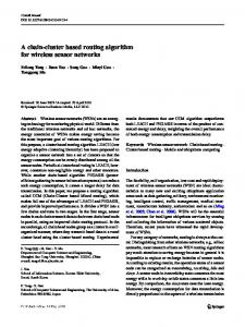
of load balancing schemes to avoid the formation of hot spots, or at least reduce the significance of the problem and avoid ruining the energy conservation. The availability of multiple routes to the sink depends on the topology of the network and its surroundings and is constrained by the radio hardware characteristics. In the best possible load balancing scenario, all sensor nodes can reach the base station directly in one hop and only send what they generate. At the opposite end of the load balancing spectrum, one particular relay or a small number thereof may be the only way for sensor nodes to reach the base station, thus forming a topological bottleneck, thereby resulting in early network partitioning. Figure 1 explains how the closer a node is to the base station, the higher its workload. Each relay or parent sensor node is a topological bottleneck with respect to the upstream or children sensor nodes.
FIGURE 1. Sensor Network with Nearest Neighbor Routing.
Various energy-efficient paradigms and strategies have been devised to collect and route the data packets towards the base station, trying to maximize the lifetime of sensor nodes while maintaining system performance and operational fidelity. According to the literature, the communication among sensor nodes consumes a large portion of the battery energy of the sensor nodes, some approaches focus on reducing communication power consumption, such as clustering algorithms, data-centric paradigms, and dynamic transmission power adjustment [3]. In the presence of topological bottleneck created synthetically as a drawback of a routing strategy, energy efficient load balancing scheme may provide significant lifetime gains through a more efficient redistribution of the traffic workload. However, regardless of the routing strategy, the mainstream sensor nodes closer to the base station have to forward more packets than the ones at the periphery of the network. The heavier workload results in more energy consumption and the nodes close to the base station will deplete their energy first, leading to an early loss of connectivity in the sensor network. This problem may severely reduce the effective network lifetime. To overcome this undesirable effect, a mechanism to balance the energy usage among sensor nodes is required. The load balancing routing LBR
algorithm aims to prolong network lifetime by considering cross-layer design to equally utilize the energy between relay sensor nodes. However, the metric used to determine the network lifetime is also application dependent. The LBR algorithm assumes that the network is homogeneous but not all nodes are equally important. It considers network lifetime as the time until the first critical sensor node (relay node) dies and runs out of its energy supply, or network partitioning occurs. Using computer simulations, the WSN is proposed to be homogeneous tree-like network deployed randomly with stationary sensor nodes and perimeter base station, and is operating in an event-driven mode as in structural health monitoring or environmental monitoring paradigms.
SYSTEM MODEL Deriving WSN lifetime model has been studied in the literature based on different definitions such as the spatial behavior of the source sensor nodes, sensing coverage and network connectivity [1-6]. The upper bounds on the network lifetime have been derived by considering the spatial behavior of the data source [1]. To achieve this goal, a simplified version is initially considered where the data source is a specific point, and the source is connected to the sink with a straight line consisting of relaying sensors. This work has been extended to the networks whose nodes may perform different tasks of sensing, relaying and aggregating [2]. The load balancing routing (LBR) algorithm employs local neighboring information to allow nodes to quickly find a new parent upon parent loss using. In LBR, a sensor network consists of, randomly deployed, static homogeneous sensor nodes with single stationary perimeter base station that periodically retransmits route advertisements so that the routing tree is continuously maintained, where the routing algorithm is fully distributed, in that each sensor node makes individual routing decisions based on locally collected information. Sensor nodes communicate immediately with other sensor nodes and the base station if they are within their radio transmission range as shown in figure 2 using a CSMA-based MAC protocol (e.g., IEEE802.15.4). Sensor nodes estimate their residual energy level of their batteries at any time and estimate the energy consumed and their link quality with their neighbors. Since the predominant traffic in the network is many-to-one data traffic from sensor nodes to base stations, sensor nodes can perform data aggregation to minimize energy consumed for data transmissions. In the literature [5-12], the meaning of network lifetime has many definitions according to the sensor network’s application and/or deployment topology as a lifetime has a great significance in the design of WSNs. Lifetime of a sensor network can be generally defined as the time after which certain fraction of sensor nodes run out of their batteries, resulting in a routing hole or hot spot within the network or the time duration that the network is operational and can perform its assigned task. In addition to that, network lifetime depends typically on other factors such as the region of observation, the source behavior within that region, base station location, number of nodes, radio path loss characteristics and network connectivity, efficiency of sensor node electronics and the energy available on a sensor node [13-18].
FIGURE 2. Homogeneous Sensor Nodes with Fixed Transmission Powers.
Importance of Sensor Node’s Location In other words, network lifetime is the time span from the deployment to the instant when the network is considered non-functional. It can be, for example, the time when the base station no longer receives data packets from the source sensor nodes, or no feasible paths from the source sensor nodes to the base station [13]. Figure 3 shows how the location and the importance of different sensors could affect network lifetime. In the figure, the red nodes represent the sensors that have run out of energy and the white ones denote the ones that are still alive. In both Figure 3(a) and (b) the sensor network cannot act as it suppose to do since in both cases the sensor network cannot gain data from some sensors, but in Figure 3(a), although there are only three failed relay sensor nodes, the base station cannot get data from most of these sensor nodes. And in Figure 3(b), there are a small number of dead sensor nodes (e.g., four dead sensor nodes), but the base station can still get data from most of the sensors in the sensor network. So the damage to the sensor network by failed sensor nodes is not only related to the number of failed sensor nodes but also related to the location of failed sensor nodes. To this end, sensor nodes in the sensor network have different importance. Each sensor node is biased to count the importance of its parent sensor node. Based on above analysis, the closer the sensor node to the base station, the more important and the more critical it is. The transmitter power level of the sensor node should be adjusted to the minimum level appropriate for the intended receiver within the transmission range [13].
FIGURE 3. Importance of Deployed Sensor Nodes.
If assumed that a path loss occurs in the sensor energy model according to the attenuation model for free space propagation [1,3,4]. Therefore, the weight or importance w i of any sensor node Si can be modeled based on the squared distance d 2 from the base station as in Eq. 1.
1 wi = a 2 d
(1)
where, a = signal attenuation coefficient. 1 = Path loss d2
Energy Dissipation Model in Multihop Routing Since malfunctioning of some critical relay sensor nodes due to power failure or physical damage can cause significant topological changes and may require network reorganization, it is very important to minimize energy consumption of each individual sensor node in order to maximize lifetime. As a result, lifetime analysis at the sensor node level is performed and discussed using simulation. To this end, the lifetime of an individual sensor node as a critical relay node is modeled based on the workload and the energy dissipation model in the sensor node. Since the lifetime of the multi-hop networks is dependent on the used routing strategy, the lifetime estimation is derived in relation to the proposed load balancing routing algorithm (LBR). A typical wireless sensor node has a sensing system, A/D conversion circuitry, DSP and a radio transceiver. The sensing system is an application dependent and the communication components are most consumer of the energy. A simple first order radio model for a wireless Channel is shown in figure 4 [19]. The energy dissipation model is developed mathematically for the lifetime of a sensor network when the energy dissipation and the workload within the network are balanced between critical relay sensor nodes. Using this model, an energy efficient load balancing routing algorithm is developed to achieve a best possible network lifetime through simulations using Matlab®.
FIGURE 4. Wireless Channel Model.
The total energy dissipation per senor node for transmitting a packet of n bits over one hop wireless link can be expressed as in Eq. 2 and Eq.3 respectively.
ETotal _ TX = ETX [n, d ] + PT Tst + Eencoding
(2)
ETX [ n, d ] = n eTC + n e Amp d α = h + c d α
(3)
where, PT
= power consumption of the transmitter circuitry in startup time.
Tst
= startup time of the transceiver (MAC protocol dependent).
Eencoding n
= energy used to encode transmitted data packets. = packet length in bits.
d
= distance between transmitter and the intended receiver node.
eTC
= energy dissipated by the transmitter circuitry per bit.
e Amp α c h
= energy used to run the transmitter amplifier per bit over distance d. = path loss exponent. = path loss coefficient. = overhead energy for a packet transmission.
The total energy dissipation per sensor node for receiving a packet of n bits over one hop wireless link can be expressed as in Eq. 4 and Eq. 5 respectively.
ETotal _ RX = E RX [ n] + PR Tst + E decoding
(4)
E RX [ n ] = n ∗ e RC
(5)
where, PR
= power consumption of the receiver circuitry in startup time.
Edecoding
= energy used to decode received data packets.
eRC
= energy dissipated by the receiver circuitry per bit.
The effect of the transceiver startup time, Tst, depends greatly on the type of MAC protocol used. To minimize power consumption it is desired to have the transceiver in a sleep mode as much as possible however constantly turning on and off the transceiver also consumes energy to bring it to readiness for transmission or reception. eTC, eAmp, and eRC are hardware dependent parameters. The path loss exponent α depends on the local terrain and is determined by empirical measurements. The typical value of α for WSNs varies from 2 (e.g., free space propagation model) to 4 (e.g., multipath fading channel models) [18]. Typically, there are two possible transmission power scenarios: Variable/adjustable and fixed/constant transmission power. If the transmitter is capable of adjusting its signal power level depending on the distance of the intended receiver from the transmitter such that the power consumed in transmission is minimized as possible, the transmission energy model is called variable. While in constant transmission energy model, the transmitter transmits at the same fixed power level irrespective of the distance between the transmitter and the intended receiver while the transmitter’s radio uses a fixed power for all transmissions. In the work of this chapter, fixed transmission power is considered because several commercial radio interfaces have a very limited capability for dynamic power adjustments even though the adjustable transmission power could benefit the network lifetime. In this case, the transmission energy dissipated per bit in an individual sensor node α is fixed to a certain value of ( eamp d ) at the transmitter node. It is also assumed that a constant amount of energy is consumed in internal computations and processing of data packets (e.g., encoding and/or decoding) while considering the energy consumed in a transmitting power is proportional to the square of the distance (e.g., free space) between transmitter and the intended receiver node [14,19], and the energy consumed in an amplifying the signal to achieve acceptable signal to noise ratio (S/N)r at the receiver sensor node. In other words, to model the energy dissipation per relay sensor node in multihop network merely to the actual communication process (transmitting and/or receiving), the energy spent in encoding, decoding, as well as on the transceiver startup is not considered in the simulations analysis as shown in figure 5. The energy consumption calculation needs to be solved periodically to account for the residual energy of sensor nodes. This will be used in the parent/path selection process of the proposed routing algorithm. For simplicity, it is initially assumed that there is one data packet of n-bits being relayed from the source sensor node towards the base station.
FIGURE 5. Data Packets Relayed through Multihop Network.
The total energy dissipated by any parent sensor node to relay a packet of n-bits from source sensor node toward the base station can be combined from Eq. 3 and Eq. 5 to form Eq. 6.
Ei , Re lay = n (eTC + eRC + eamp ∗ diα )
(6)
For leaf or source sensor nodes at which the data packets were originated, the energy dissipated by the receiver circuitry per bit eRC is assigned to zero. The current residual energy level of sensor node after relaying one packet of n-bits can be calculated by deducting the initial or the previous energy value from the value of the energy dissipated by sensor node i by Eq. 7.
Ei , residual = Ei ,initial − Ei ,relay
(7)
The energy consumption of relay sensor node measures the average energy dissipated by this node in order to relay (transmit and/or receive) a data packet from the source sensor node to the base station. The similar metric is used in the work on directed diffusion [20] to indicate the energy efficiency level of WSNs. This metric gives an indication of the network state in terms of energy consumption. It is calculated as follows from Eq. 8. M
Average Dissipated Energy =
∑E i =1
i , relay
M *N
where, M = the total number of operational sensor nodes in the network. N = the amount of data packets received by the base station.
(8)
LOAD BALANCING ROUTING Related Work The minimum cost-based routing (e.g., using minimum number of hops) and the reliability-oriented routing (e.g., using the optimal link state) are typically used in wireless networks. One of the simplest ways to make multihop routing is flooding broadcast packets to all connected sensor nodes in the network but it is not suitable for busy traffic network and does not guarantee the maximum lifetime in the network [12]. Alternatively, the lifetime-aware routing (e.g., using minimum required energy) attempts to prolong network lifetime by distributing the workload among the relay nodes [21, 22]. Though this scheme may not have the minimum overall consumed energy [12]. In mote-dominated WSNs, Berkeley MintRoute (MInimum Number of Transmissions) [23, 24], MultihopLQI [25] and Collection Tree Protocol (CTP) [26] are the most popular reliability-oriented, tree-based collection multihop routing protocols. While the original MintRoute protocol was designed for Mica1 and Mica2 motes as a part of the official TinyOS distribution, the newer version of MintRoute, MultihopLQI [26], was designed to support CC2420-(802.15.4)-based motes like MicaZ and Telos [27]. There are two major differences between MultihopLQI and MintRoute. Firstly, MultHopLQI uses the Link Quality Indicator (LQI) provided by the radio hardware instead of link estimator using Received Signal Strength Indicator (RSSI) to estimate link quality to its neighbors as in MintRoute. Secondly, MultihopLQI maintains only a state for one parent node at a time, neither routing tables nor blacklisting are used as in MintRoute, and a new parent is adopted if it advertises a lower cost than the current parent. Link Quality Information is used as a link metric with Channel State Information (CSI) to obtain the cost of a given route. MultihopLQI avoids routing tables by only keeping state for the best parent at a given time; this measure drastically reduces memory usage and control overhead. MultihopLQI uses a constant rate for transmitting beacons. The rate of the current implementation of MultihopLQI is fixed at one beacon every 32 seconds. Hence, the energy dissipation cost of MultihopLQI protocol is only a function of the data rate. The size of each control packet size is 12 bytes and the data packets have eight bytes header. The most recent protocol of MintRoute, Collection Tree Protocol (CTP) [26], designed to support sensor networks with multiple base stations. CTP uses adaptive beacon rate. In terms of energy dissipation cost, MultihopLQI performs better than CTP and MintRoute. However, none of the aforementioned routing protocols explicitly apply load balancing in their routing schemes. As a result, this chapter focuses on balanced energy dissipation model for lifetime maximization by taking the advantage from reliability-oriented routing schemes, i.e., MultiHopLQI collection protocol [25], and maximum lifetime routing schemes, i.e., Energy-Aware Routing (EAR) protocol [28].
PERFORMANCE EVALUATION This section describes the used methodology to evaluate the operation of a WSN using the proposed routing algorithm and to benchmark LBR against a wellestablished, well-tested, and highly used collection protocol that is part of the TinyOS release. Since TinyOS 2.x and TinyOS 1.x have different packet scheduling and MAC layer, LBR is compared with the TinyOS 2.1 implementation of MultiHopLQI, the state-of-the art collection routing protocol [25], which is an updated version of the MintRoute protocol [23,24] and is a component library in TinyOS 2.x, then considers the impact of network routings on energy efficiency, load balancing, and the entire network lifetime. As MultiHopLQI has been used in recent real sensor networks deployments, such as in [26], [29], and [30], it is considered a reasonable comparison.
Simulation Settings Simulations were implemented in Matlab® using a maximum number of 100 sensor nodes deployed randomly in a sensor field of 100x100 meters square with a single stationary base station. The base station is deployed on the periphery of the sensor field to increase the network depth. Each sensor node has a constant transmission range and uses a constant rate of one beacon per second for transmitting route maintenance control beacons. The maximum link layer packet size is taken from the default maximum packet transferable using TinyOS 2.x with CC2420, which is 29 bytes. Performance comparisons were conducted between the proposed load balancing scheme and the benchmark scheme, MultiHopLQI. To minimize the variations on routing performance from MAC layer, no energy conservation strategy is introduced in the MAC protocol. By this, the most conservative measurements are tending to be given on the advantages of energy conservation routing strategy for LBR over the benchmark scheme. The experiments were run seven times for 300 seconds and the consistent obtained results were averaged. All sensor nodes have the same initial energy level. The rates at which the data packets are transferred to the base station and the amount of energy required getting the data packets relayed toward the base station were tracked. All sensor nodes start up with the same initial energy level of one energy unit at the beginning of each simulation while assuming the base station can have its persistent energy supply as is usually the case in real WSN applications. Since the sensor nodes have limited energy levels, they use up this available energy during the simulation period. Once a sensor node runs out of energy, it is considered dead and can no longer transmit or receive any data or control packets. The wireless medium was simulated by means of the free space propagation model [31]. Moreover, it is assumed that the experiments follow an event-driven model and the source sensor nodes detect related stimulus (e.g., alteration of gas pipeline pressure). Therefore, sensed data can be aggregated. Each source sensor node generates data packets and sends them to the base station through the network with a fixed date rate.
Simulation Results Operational Network Lifetime Figure 6 shows the time when the residual energy levels of sensor nodes drain-out and how the sensor network becomes disconnected when all the sensor nodes which can relay data packets toward the perimeter base station have died. From figure 6, it can be observed that LBR performs better than MultihopLQI as the lifetimes of individual sensor nodes have been maximized. MultihopLQI protocol balances the traffic load using different paths occasionally as a direct effect of LQI values in the route selection, thereby resulting in a balanced energy consumed by few relay sensor nodes. The workload through other sensor nodes can be sub-optimal which significantly increases their residual energy dissipation in rerouting upstream data packets. Therefore, in MultihopLQI, many heavily loaded sensor nodes along the routing path die in a short period of time and the total number of sensor nodes that die is very high, while lightly loaded sensor nodes die very late. These lightly loaded sensor node are much fewer. On the other hand, LBR conveys data packets through sensor nodes with higher residual energy levels, thus the least number of nodes are dead during the same period of time. LBR balances the energy consumption by periodically updating energy efficient routes. As the residual energy of an individual sensor node decreases to the threshold, the cost of using outgoing links from that sensor node increases. The network lifetime with load balancing routing has a substantial increase of approximately three times than MultiHopLQI routing. It can also be observed that the number of dead sensor nodes with load balancing routing rises gradually with time than the benchmark routing protocol. It obviously demonstrates that load balancing routing scheme can maximize the network lifetime. Since dynamic transmission power adjustment paradigm reduced the transmission power consumption, the lifetimes of sensor nodes in variable transmission energy model could be longer than double the lifetimes of nodes in a constant transmission energy model [32,33]. Clearly, equipping sensor nodes with power control transmitters can increase lifetimes of sensor nodes. The energy consumed in processing and receiving a packet is independent of the distance between the transmitter and the receiver. Therefore, actual increase in the lifetime depends on the energy dissipated by the transmitter amplifier, which is proportional to the distance between the transmitter and the attended receiver. Studying network lifetime with variable transmission power has been left for future work as it is out of the scope of the chapter. Figure 7 shows that the network lifetime has a deteriorating trend as the node density increases due to an abundance of control and data packets that are retransmitted throughout the sensor network. Comparing with the benchmark scheme, the network lifetime with load balancing routing has a substantial increase of 20-30% than MultiHopLQI routing. It can be also seen that the network lifetime with load balancing routing degrades more gracefully and it is more stable than MultiHopLQI routing protocols when the node density increases.
FIGURE 6. Lifespan of Individual Sensor Nodes
FIGURE 7. Average Network Lifetime
Since the path selection in MultiHopLQI routing protocol does not consider the node energy level in the route selection process, the load balancing routing algorithm has a greater network lifetime than MultiHopLQI. In MultiHopLQI, the large number of redundant data packets copies that are retransmitted between different sensor nodes rapidly deplete the available energy.
Average Dissipated Energy Figure 8 illustrates the relationship between the average dissipated energy during network operation and the density of the sensor field. As an overall trend it can be seen that the averaged dissipated energy by the sensor nodes in both routing algorithms has an increasing trend as the network density becomes high for the same squared sensor field size. Comparing with MultihopLQI, LBR performs quite well where the energy consumption increases steadily with the size of the neighboring nodes. In contrast, the MultihopLQI dissipate more energy for the same network size and the energy dissipation augment considerably after escalating the node density by 50 sensor nodes. It demonstrates that LBR routing scheme outperform MultihopLQI with the variation of the network density. To study the influence of network densities on energy consumption, evaluations under various densities are conducted. Different scenarios with 10–100 sensor nodes were deployed arbitrarily in a fixed 100x100 meters square sensor field area, in increments to 30, 50, 70, and 100 nodes. Figure 9 shows the change in the node’s average residual energy level after a period of data transmission. It is apparent that the network density has an impact on the individual node’s residual energy level. As an overall trend, the average remaining energy level decreases with higher density. MultiHopLQI cannot reduce the redundant data copies in the network which resulted by a high traffic load handled by each individual forwarding node. This makes the average remaining energy level for MultiHopLQI to degrade much faster than the load balancing routing mechanism which keeps a balanced network workload towards the base station to maintain balanced energy dissipation.
FIGURE 8. Average Dissipated Energy
FIGURE 9. Nodal Residual Energy Ratio
Packet delivery ratio This metric is the percentage amount of all unique injected and aggregated packets from randomly selected source sensor nodes and received by the base station [34]. Figure 10 shows that LBR outperforms the MultiHopLQI and delivers obviously a higher percentage of packet delivery rates in all load scenarios. This is due to the random selection of source nodes and the implementation of data packets aggregation. MultihopLQI maintains a relatively steady packet delivery rate for all load scenarios. The consistent packet delivery rates for LBR in the random network show its scalability and reliability. In LBR, the average packet delivery rate is approximately 76% while in MultihopLQI; the packet delivery rate is moderately lower by 21%. The random topology was simulated with an assumption that when the node transmits a packet, it has a 90% chance of being successfully delivered to the next hop or the selected parent node. This doesn’t accurately reflect the observation that some packets are skipping over the intended node as experienced in [13]. In the end, the simulation results show that the packet delivery rates are much higher than the experimental results because the simulation links are based on connectivity matrix and do not consider the signal attenuation [31].
FIGURE 10. Packet Delivery Ratio
CONCLUSION In this chapter, an energy-efficient load-balancing routing algorithm has been presented and benchmarked with the state-of-the art reliability-oriented collection protocol. The proposed algorithm incorporates the residual energy of the relay nodes with the link state in the parent selection decision to distribute the load among the sensor nodes in order to prolong the entire network lifetime. The results show that energy balance is advantageous for network lifetime extension. Through intensive simulations in Matlab®, the feasibility of the load balancing scheme is shown by demonstrating the improved network lifetime in several deployment scenarios. Additionally, it has been observed that significant advantages can be obtained by designing and implementing a routing algorithm for WSNs with an integrated energy-wise load balancing scheme. This useful information will be used for the parent selection for the converge-cast routing tree to keep the workload balanced along the routing path.
REFERENCES 1. 2. 3. 4. 5. 6. 7. 8. 9. 10. 11. 12. 13. 14.
networks,” IEEE International Conference on Communications, Communications (ICC’01). vol. 3, Helsinki, Finland, 2001, pp. 785–790. M. Bhardwaj and A. P. Chandrakasan, “Bounding the lifetime of sensor networks via optimal role assignments,” the 21st Annual Joint Conference of the IEEE Computer and Communications Societies (INFOCOM 2002), vol. 3, 2002, pp. 1587–1596. Wendi Rabiner Heinzelman, Amit Sinha, Alice Wang, and Anantha P. Chandrakasan, “Energy-Scalable Algorithms and protocols for Wireless Microsensors Networks,” (ICASSP’00), 2000. J. G. Proakis and M. Salehi, Communication Systems Engineering, 2nd edition, Upper Saddle River, NJ, USA: Prentice-Hall, 2004. H. Zhang and J. Hou, “On deriving the upper bound of lifetime for large sensor networks,” the 5th ACM international symposium on Mobile ad hoc networking and computing (MobiHoc’04), New York, NY, USA, ACM Press, 2004, pp. 121–132. V. Rai and R. N. Mahapatra, “Lifetime modeling of a sensor network,” the conference on Design, Automation and Test in Europe (DATE’05), Washington, DC, USA, IEEE Computer Society, 2005, pp. 202–203. E. J. Duarte-Melo and M. Liu, “Analysis of energy consumption and lifetime of heterogeneous wireless sensor networks,” in IEEE Global Telecommunications Conference (GLOBECOM’02), vol. 1, Nov. 2002, pp. 21–25. Q. Xue and A. Ganz, “On the lifetime of large scale sensor networks,” Elsevier Journal on Computer Communications, vol. 29, pp. 502–510, 2006. S. Baydere, Y. Safkan, and O. D. Incel, “Lifetime analysis of reliable wireless sensor networks,” IEICE Transactions on Communications, pp. 2465–2472, 2005. Y. Chen and Q. Zhao, “On the lifetime of wireless sensor networks,” IEEE Communications Letters, vol. 9, no. 11, pp. 976–978, Nov. 2005. S. Coleri, M. Ergen, and T. J. Koo, “Lifetime analysis of a sensor network with hybrid automata modeling,” in the 1st ACM international workshop on Wireless sensor networks and applications (WSNA’02), New York, NY, USA: ACM Press, 2002, pp. 98–104. J. N. Al-Karaki and A. E. Kamal, “Routing techniques in wireless sensor networks: a survey,” IEEE [see also IEEE Personal Communications] Wireless Communications, vol. 11, no. 6, pp. 6–28, Dec. 2004. K. Daabaj, M. Dixon, T. Koziniec, “Experimental Study of Load Balancing Routing for Improving Lifetime in Sensor Networks,” the IEEE 5th Conference of Wireless Communications and Mobile Computing (WiCOM’09), Beijing, China, Sept. 24-26, 2009. W. B. Heinzelman, A. P. Chandrakasan, and H. Balakrishnan, “An application-specific protocol architecture for wireless microsensor networks,” IEEE Transactions on Wireless Communications, vol. 1, no. 4, pp. 660–670, Oct. 2002. M. Bhardwaj, T. Garnett, and A. P. Chandrakasan, “Upper bounds on the lifetime of sensor
15. R. Madan and S. Lall, “Distributed algorithms for maximum lifetime routing in wireless sensor networks,” IEEE Transactions on Wireless Communications, vol. 5, no. 8, pp. 2185–2193, Aug. 2006. 16. J.-H. Chang and L. Tassiulas, “Energy conserving routing in wireless ad-hoc networks,” in IEEE INFOCOM ’00, Tel-Aviv, Israel, Mar. 2000, pp. 22–31. 17. Y. Xu, J. Heidemann, and D. Estrin, “Geography-informed energy conservation for ad hoc routing,” in the 7th annual international conference on Mobile computing and networking (MobiCom’01), New York, NY, USA: ACM Press, 2001, pp. 70–84. 18. E. I. Oyman and C. Ersoy, “Multiple sink network design problem in large scale wireless sensor networks,” in the IEEE International Conference on Communications (ICC’04), vol. 6, June 2004, pp. 3663–3667. 19. W. Heinzelman, A. Chandrakasan, and H. Balakrishnan, “Energy efficient communication protocol for wireless micro-sensor networks,” in the 33rd Hawaii International Conference on System Sciences (HICSS ’00), Maui, Hawaii, Jan. 2000, pp. 3005 – 3014. 20. Chalermek Intanagonwiwat, Ramesh Govindan, and Deborah Estrin. “Directed diffusion: a scalable and robust communication paradigm for sensor networks,” in the 6th Annual ACM International Conference on Mobile Computing and Networking (MobiCom), pages 56–67, 2000. 21. Arvind Sankar and Zhen Liu, “Maximum Lifetime Routing in Wireless Ad-hoc Networks,” IEEE INFOCOM 2004. 22. Joongseok Park Sartaj Sahni, “Maximum Lifetime Routing in Wireless Sensor Networks,” Computer & Information Science & Engineering, University of Florida June 2, 2005. 23. Woo, T. Tong, and D. Culler, “Taming the Underlying Challenges of Reliable Multihop Routing in Sensor Networks,” in the 1st International Conference on Embedded Networked Sensor Systems (SenSys’03), Los Angeles, CA, USA, November 2003. 24. Woo and T. Tong. Tinyos mintroute collection protocol. http://www.tinyos.net/tinyos-1.x/tos/ lib/MintRoute, 2004. 25. Tinyos multihoplqi collection protocol.http://www.tinyos.net/tinyos-1.x/tos/lib/MultiHopLQI/. 26. O. Gnawali, R. Fonseca, K. Jamieson, D. Moss, and P. Levis, “Collection Tree Protocol,” in the 7th ACM Conference on Embedded Networked Sensor Systems (SenSys’09), 2009. 27. Chipcon Inc., CC2420 data sheet. http://focus.ti.com/lit/ds/symlink/cc2420.pdf. 28. R. Shah, J. Rabaey, “Energy aware routing for low energy ad hoc sensor networks,” IEEE WCNC’02, Orlando, FL, March 2002; 350–355. 29. M. Wachs, J. Choi, J. Lee, K. Srinivasan, Z. Chen, M. Jain, and P. Levis, “Visibility: A New Metric for Protocol Design,” in the Fifth ACM Conference on Embedded Networked Sensor Systems (SenSys’07), Sidney, Australia, November 2007. 30. G. Werner-Allen, K. Lorincz, J. Johnson, J. Lees, and M. Welsh, “Fidelity and Yield in a Volcano Monitoring Sensor Network,” in USENIX Symposium on Operating Systems Design and Implementation, Seattle, WA, Nov. 2006. 31. T. S. Rapport, “Wireless Communications: Principles and Practice,” Prentice Hall, 1992. 32. Jae-Hwan Chang and Leandros Tassiulas, “Maximum lifetime routing in wireless sensor networks,” IEEE/ACM Transactions on Networking, 12(4):609–619, 2004. 33. Alaa Muqattash and Marwan M. Krunz, “A distributed transmission power control protocol for mobile ad hoc networks,” IEEE Transactions on Mobile Computing, 3(2):113–128, 2004. 34. Jerry Zhao, Ramesh Govindan, “Understanding Packet Delivery Performance in Dense Wireless Sensor Networks,” ACM SenSys'03, Los Angeles, California, USA, November 5-7, 2003.