and ALE (stirring zone) descriptions for the different computational ... Friction stir welding (FSW) is a solid state joining technology in which no gross melting.
Local and global approaches to Friction Stir Welding N. Dialami, M. Chiumenti, M. Cervera and C. Agelet de Saracibar International Center for Numerical Methods in Engineering (CIMNE) Universidad Politécnica de Cataluña c/ Gran Capitán s/n, Módulo C1, Campus Norte UPC, 08034 Barcelona, Spain
Keywords:
Friction Stir Welding Process, visco-plasticity, particle tracing, stabilized …nite element method, ALE formulation, residual stresses
Abstract This paper deals with the numerical simulation of Friction Stir Welding (FSW) processes. FSW techniques are used in many industrial applications and particularly in the aeronautic and aerospace industries, where the quality of the joining is of essential importance. The analysis is focused either at global level, considering the full component to be jointed, or locally, studying more in detail the heat a¤ected zone (HAZ). The analysis at global (structural component) level is performed de…ning the problem in the Lagrangian setting while, at local level, an apropos kinematic framework which makes use of an e¢ cient combination of Lagrangian (pin), Eulerian (metal sheet) and ALE (stirring zone) descriptions for the di¤erent computational sub-domains is introduced for the numerical modeling. As a result, the analysis can deal with complex (non-cylindrical) pin-shapes and the extremely large deformation of the material at the HAZ without requiring any remeshing or remapping tools. A fully coupled thermo-mechanical framework is proposed for the computational modeling of the FSW processes proposed both at local and global level. A staggered algorithm based on an isothermal fractional step method is introduced. To account for the isochoric behavior of the material when the temperature range is close to the melting point or due to the predominant deviatoric deformations induced by the visco-plastic response, a mixed …nite element technology is introduced. The Variational Multi Scale (VMS) method is used to circumvent the LBB stability condition allowing the use of linear/linear P1/P1 interpolations for displacement (or velocity, ALE/Eulerian formulation) and pressure …elds, respectively. The same stabilization strategy is adopted to tackle the instabilities of the temperature …eld, inherent characteristic of convective dominated problems (thermal analysis in ALE/Eulerian kinematic framework).
1
At global level, the material behavior is characterized by a thermo-elasto- viscoplastic constitutive model. The analysis at local level is characterized by a rigid thermo-visco-plastic constitutive model. Di¤erent thermally coupled (non-Newtonian) ‡uid-like models as Norton-Ho¤, Carreau or Sheppard-Wright, among others are tested. To better understand the material ‡ow pattern in the stirring zone, a (Lagrangian based) particle tracing is carried out while post-processing FSW results. A coupling strategy between the analysis of the process zone nearby the pin-tool (local level analysis) and the simulation carried out for the entire structure to be welded (global level analysis) is implemented to accurately predict the temperature histories and, thereby, the residual stresses in FSW.
1
Introduction
1.1
Industrial background of FSW
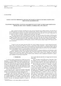
Friction stir welding (FSW) is a solid state joining technology in which no gross melting of the welded material takes place. It is a relatively new technique (developed by The Welding Institute (TWI), in Cambridge, UK, in 1991) widely used over the past decades for joining aluminium alloys. Recently, FSW has been applied to the joining of a wide variety of other metals and alloys such as magnesium, titanium, steel and others. FSW is considered to be the most signi…cant development in metal joining in decades and, in addition, is a "green" technology due to its energy e¢ ciency, environmental friendliness, and versatility. This process o¤ers a number of advantages over conventional joining processes (such as e.g. fusion welding). The main advantages, often mentioned, include: (a) absence of the need for expensive consumables such as a cover gas or ‡ux; (b) ease of automation of the machinery involved; (c) low distortion of the work-piece; and (d) good mechanical properties of the resultant joint [91], [120]. Additionally, since it allows avoiding all the problems associated to the cooling from the liquid phase, issues such as porosity, solute redistribution, solidi…cation cracking and liquation cracking are not encountered during FSW1 . In general, FSW has been found to produce a low concentration of defects and is very tolerant to variations in parameters and materials. Furthermore, since welding occurs by the deformation of material at temperatures below the melting temperature, many problems commonly associated with joining of dissimilar alloys can be avoided, thus high-quality welds are produced. Due to this fact, it has been widely used in di¤erent industrial applications where metallurgical characteristics should be retained, such as in aeronautic, naval and automotive industry. During FSW, the work-piece is placed on a backup plate and it is clamped rigidly to eliminate any degrees of freedom (Figure 1). A nonconsumable tool, rotating at a constant speed, is inserted into the welding line between two pieces of sheet or plate material (which are butted together) and generates heat. This heat is produced, on one hand, by the friction 1
However, it must be noted that, as in the traditional fusion welds, there also exist a softened heat a¤ected zone (HAZ) and a tensile residual stress parallel to the weld.
2
Figure 1: FSW process.
between the tool shoulder and the work-pieces, and, on the other hand, by the mechanical mixing (stirring) process in the solid state. This results in the plasti…cation of the material close to the tool at very high strain rates and leads to the formation of the joint. In detail, the plasticized material is stirred by the tool and the heated material is forced to ‡ow around the pin tool to its backside thus …lling the hole in the tool wake as the tool moves forward. As the material cools down, a solid continuous joint between the two plates emerges. Usually the tool is tilted at an angle of 1 3o away from the direction of travel, although some tool designs allow it to be positioned orthogonally to the work-piece (Figure 2). The welding tool consists of a shoulder and a pin. The length of the pin tool is slightly less than the depth of weld and the tool shoulder is kept in close contact with the work-piece surface (see Figure 3). The tool serves three primary functions, that is, heating of the work-piece, movement of material to produce the joint (stirring), and containment of the hot metal beneath the tool shoulder. The function of the pin tool is to heat up the weld metal by means of friction and plastic dissipation, and, through its shape and rotation, force the metal to move around its form and create a weld. The function of the shoulder is to heat up the metal through friction and to prevent it from being forced out of the weld. The tool shoulder restricts metal ‡ow to a level equivalent to the shoulder position, that is, approximately to the initial work-piece top surface. Depending on the geometrical con…guration of the tool, material movement around the pin can become complex, with severe gradients in temperature and strain rate. This environment creates a challenge for modelers due to the resulting coupled thermo-mechanical nature, the large deformation and strain rates near the pin. Since FSW is not a symmetric process, two sides of the tool are di¤erentiated. One can see in Figure 4 that the work-pieces being joined by the weld are either on the retreating or advancing side of the rotating tool. The retreating side is the one where the tool rotating direction is opposite to the tool moving
3
Figure 2: Tilt angle in FSW
Figure 3: Schematic representation of the friction stir welding process
4
Figure 4: De…nition of Friction Stir Welding zones [54]
direction and parallel to the metal ‡ow direction. In contrast, the advancing side is the one where the tool rotation direction is the same as the tool moving direction and opposite to the metal ‡ow direction. This unsymmetric nature results in a di¤erent material ‡ow on the di¤erent sides of the tool and has a large e¤ect on many applications, especially lap joints [27]. The periodic "onion ‡ow" pattern that is left behind as the tool advances is schematically illustrated in Figure 4. During the early development of FSW, the process appeared simple, compared to many conventional welding practices. However, as development continued, the complexity of FSW was realized. It is now known that properties following FSW are a function of both controlled and uncontrolled variables (response variables) as well as external boundary conditions. For example, investigators have now illustrated that post-weld properties depend on: Tool travel speed: in‡uences total heat, porosity and weld quality. Tool rotation rate: in‡uences total heat and weld quality. Tool design: shoulder diameter, scroll or concave shoulder, features on the pin and pin length in‡uence the extent of the material (Figure 5). Tool tilt: It in‡uences the contact pressure. There exists lower contact pressure (or incomplete contact) on the leading edge of the shoulder due to tool tilt (typically between 0 and 3 ). Material thickness: in‡uences cooling rate and through-thickness temperature gradients. 5
Figure 5: Di¤erent pin shapes.
These parameters must be carefully calibrated according to the welding process and the selected material, respectively. The strong coupling between the temperature …eld and the mechanical behavior is the key-point in FSW and its highly non-linear relationship makes the process setup complex. The operative range for most of the welding process parameters is rather narrow requiring a tedious characterization and sensitivity analysis. This is why, despite the apparent simplicity of this novel welding procedure, computational modeling is considered a very helpful tool to understand the leading mechanisms that govern the material behavior, attracting more and more the research interest. Finite element modeling is an option which can help to determine process parameters that would otherwise require further experimental testing for validation and analysis. The weld quality depends largely on how the material is heated, cooled and deformed. Hence a prior knowledge of the temperature evolution within the work-piece would help in designing the process parameters for a welding application. Research in the …eld of FSW joints has been limited possibly due to proprietary publishing restriction within industry. For this reason, Finite Element Analysis (FEA) could be also very bene…cial. Two process parameters of interest for FSW welds are tool travel rates and rotational tool velocities. With respect to this, a lot of emphasis has been laid on FEA analysis, as it may broaden the scope of application of FSW. Another important process parameter in FSW is the heat ‡ux. This can be also easily included in the FEA. The heat ‡ux should be high enough to keep the maximum temperature in the work-piece around 80% to 90% of the melting temperature of the work-piece material, so that welding defects are avoided [33]. Moreover, analytical and numerical methods have a role to play, although numerical methods dominate due to the accuracy and ease-to-use of modern workstations and software. Numerical modeling is based on discretized representations of speci…c welds, using …nite element, …nite di¤erence, or …nite volume techniques. These methods can capture much of 6
the complexity in material constitutive behavior, boundary conditions, and geometry, but in practice, a limited range of conditions tends to be studied in depth. Therefore, it is good modeling practice to explore simpli…cations to the problem that give useful insight across a wider domain, for example, making valid two-dimensional (2-D) approximations to inherently three dimensional (3-D) behavior. It is also essential to deliver a model that is properly validated and whose sensitivity is known to uncertainty in the input material and process data— ideals that are rarely carried through in practice.
1.2
Challenges for the simulation of FSW process
Information about the shape, dimensions and residual stresses in a component after welding and mechanical properties of the welded joint are of great interest in order to improve the quality and to prevent failures during manufacturing or in service. The FSW process can be analyzed either experimentally or numerically. FSW is di¢ cult to analyze experimentally; however, process parameters and di¤erent …xture set-ups can be evaluated without doing a large number of experiments. An experiment can be designed to answer one or more carefully formulated questions. The goals must be clari…ed perfectly to choose the appropriate parameters and factors. Otherwise the goal is not achieved and the experiment must be repeated. Di¤erent welded specimens are produced by varying the process parameter. The properties and microstructure changes in weld are investigated. For instance, the tensile strength of the produced joint is tested at room temperature. Microstructure of the weld is analyzed by means of optical microscopy or microhardness measurements. The alternative to the experimental FSW analysis is numerical modeling and simulation. Computer-based models provide the opportunity to improve theories of design and increase their acceptance. Simulations are useful in designing the manufacturing process as well as the manufactured component itself. To do an appropriate modeling, the physics of the problem must be well-understood. 1.2.1
Physical model
FSW simulation is a problem of complex nature; the process is highly nonlinear and coupled. Di¤erent physical phenomena occur during the welding process, involving the thermal and mechanical interactions. The temperature …eld is a function of many welding parameters such as welding speed, welding sequence and environmental conditions. Formation of distortions and residual stresses in work-pieces depend on many interrelated factors such as thermal …eld, material properties, structural boundary conditions and welding conditions. The challenging issues in physical modeling of the FSW process are divided into three parts:
7
1.2.1.1 Complex thermal behavior Heat transfer mechanisms including convection, radiation and conduction have a signi…cant role on the process behavior. Convection and radiation ‡uxes dissipate heat signi…cantly through the work-pieces to the surrounding environment while conduction heat ‡ux occurs between the work-pieces and the support. 1.2.1.2 Non-linear behavior and localized nature In FSW, the mechanical behavior is non-linear due to the high strain rates and visco-plastic material. The strong non-linear region is limited to a small area and the remaining part of the model is mostly linear. However, the exact boundaries of the non-linear zone are not known a-priori. It is generally believed that strain rate during the welding is high. Knowledge of strain rate is important for understanding the subsequent evolution of grain structure, and it serves as a basis for veri…cation of various models as well. 1.2.1.3 Coupled nature The thermal and mechanical problems are strongly coupled (the thermal loads generate changes in the mechanical …eld). The mechanical e¤ects coupled to the thermal ones include internal heat generation due to plastic deformations or viscous e¤ects, heat transfer between contacting bodies, heat generation due to friction, etc. The thermal e¤ects are also coupled to the mechanical ones; for instance, thermal expansion, temperature-dependent mechanical properties, temperature gradients in work-pieces, etc. An adequate physical model of the welding process must account for all these phenomena including thermal, mechanical and coupling aspects. 1.2.2
Numerical model
Among several numerical modeling techniques, the Finite Element (FE) framework is found to be suitable for the simulation of welding and proven to be a versatile tool for predicting a component’s response to the various thermal and mechanical loads. The FE method also o¤ers the possibility to examine di¤erent aspects of the manufacturing process without having a physical prototype of the product. To this end, a specialized thermo-mechanical coupled model needs to be implemented in a …nite element program, and the predictive capabilities of the theory and its numerical implementation must be validated. The numerical simulation of the FSW process has many complex and challenging aspects that are di¢ cult to deal with: the welding process is described by the equilibrium and energy equations governing the mechanical and thermal problems and they are coupled. Additionally, both of them are non-linear. This has important implications upon the complexity of the numerical model. Consequently, a robust and e¢ cient numerical strategy is crucial for solving such highly non-linear coupled …nite element equations. In such process, several assumptions are commonly assumed. It is important to distinguish between two di¤erent kinds of welding analyses carried out at local or global level, respectively.
8
In local level analysis, the focus of the simulation is the heat a¤ected zone. The simulation is intended to compute the heat power generated either by visco-plastic dissipation or by friction at the contact interface. At this level, the process phenomena that can be studied are the relationship between welding parameters, the contact mechanisms in terms of applied normal pressure and friction coe¢ cient, the setting geometry, the material ‡ow within the heat a¤ected zone, its size and the corresponding consequences on the microstructure evolution, etc. A simulation carried out at global level studies the entire component to be welded. In this case, a moving heat power source is applied to a control volume representing the actual heat a¤ected zone at each time-step of the analysis. The e¤ects induced by the welding process on the structural behavior are the target of this kind of study. These e¤ects are distortions, residual stresses or weaknesses along the welding line, among others. The aim of this work is to develop a robust numerical tool able to simulate the welding process considering its complex features at local level as well as global level. 1.2.2.1 Mechanical problem A quasi-static mechanical analysis can be assumed as the inertia e¤ects in welding processes are negligible due to the high viscosity characterization. At local level, the volumetric changes are found to be negligible, and incompressibility can be assumed. To deal with the incompressible behavior, a very convenient and common choice is to describe the formulation splitting the stress tensor into its deviatoric and volumetric parts. Dealing with the incompressible limit requires the use of mixed velocity-pressure interpolations. The problem su¤ers from instability if the standard Galerkin FE formulation is used, unless compatible spaces for the pressure and the velocity …eld are selected (Ladyzhenskaya-Babuška–Brezzi (LBB) stability condition). Due to this, pressure instabilities appear if equal velocity-pressure interpolations are used. Thus, the challenging issue of pressure stabilization rises up. The welding process is characterized by very high strain rates as well as a wide temperature range going from the environmental temperature to the melting point. Hence, the constitutive laws adopted should depend on both variables. The constitutive theory applied must be specialized to capture the features of the thermo-mechanically coupled strain rate and temperature dependent large deformation. According to the split of the stress tensor, di¤erent rate-dependent constitutive models can be used for modeling of the welding process. At typical welding temperatures, the large strain deformation is mainly visco-plastic. Depending on the scope of the analysis, rigid-visco-plastic or elasto-visco-plastic constitutive models can be used. Not only the prediction of the temperature evolution, but the accurate residual stress evaluation …eld generated during the process is the objective of the FSW simulation. The selected constitutive model must appropriately de…ne the material behavior and has to be calibrated by the temperature evolution. The challenge arises from the extremely non-linear behavior of these constitutive models and, therefore, from the numerical point of view, a special treatment is obligatory. Moreover, the localized large strain rates usually involved in FSW processes make the problem even more complex. 9
1.2.2.2 Thermal problem The thermal problem is de…ned by the balance of energy equation. In FSW simulation, the plastic dissipation term appearing in the energy equation has a critical role on the process behavior and it is the main source of heat generation. The de…nition of the heat source is one of the key points when studying the welding process. In global level simulations, the mesh density used to discretize the geometry is not usually …ne enough to de…ne the welding pool shape or a non-uniform heat source. This is only done if the simulation of the welding pool is the objective itself (local level analysis). If the global structure is considered, the size of the heat source is of the same dimension than the element size generally used for a thermo-mechanical analysis. Therefore, when the global model is taken into account, the resulting mesh density is usually too coarse to represent the actual shape of the heat source. Depending on the framework used to describe the formulation of the coupled thermomechanical problem, a convective term might appear in the thermal governing equations. Therefore convection instabilities of the temperature appear for convection dominated problems. It is well known that in di¤usion dominated problems, the solution is stable. However, in convection dominated problems, the stabilizing e¤ect of the di¤usion term becomes insuf…cient and oscillations appear in the temperature …eld. The threshold between stable and unstable solutions is usually expressed in terms of the Peclet number. 1.2.2.3 Kinematic framework Establishing an appropriate kinematic framework for the simulation of welding is one of the main objectives of this paper. If the welding process is studied at global level, a Lagrangian framework is an appropriate choice for the description of the problem. Lagrangian settings, in which each individual node of the computational mesh represents an associated material particle during motion, are mainly used in structural mechanics. Classical applications of the Lagrangian description in large deformation problems are the simulation of vehicle crash tests and the modeling of metal forming operations. In these processes, the Lagrangian description is used in combination with both solid and structural (beam, plate, shell) elements. Numerical solutions are often characterized by large displacements and deformations and history-dependent constitutive relations are employed to describe elasto-plastic and visco-plastic material behavior. The Lagrangian reference frame allows easy tracking of free surfaces and interfaces between di¤erent materials. In a local simulation, the main focus of the simulation is the Heat A¤ected Zone (HAZ) where the use of a Lagrangian framework is not always advantageous. In the HAZ, the large distortions would require continuous re-meshing. The alternative is to use Eulerian or Arbitrary Lagrangian Eulerian (ALE) methods. Eulerian settings are widely used in ‡uid mechanics. Here, the computational domain and reference mesh are …xed and the ‡uid moves with respect to the grid. The Eulerian formulation facilitates the treatment of large distortions in the ‡uid motion. Its handicap is the di¢ culty to follow free surfaces and interfaces between di¤erent materials or di¤erent media (e.g., ‡uid-‡uid and ‡uid-solid interfaces). 10
An Arbitrary Lagrangian Eulerian (ALE) formulation which generalizes the classical Lagrangian and Eulerian descriptions is particularly useful in ‡ow problems involving large distortions in the presence of mobile and deforming boundaries. Typical examples are problems describing the interaction between a ‡uid and a ‡exible structure and the simulation of metal forming processes. The key idea in the ALE formulation is the introduction of a computational mesh which can move with a velocity di¤erent from (but related to) the velocity of the material particles. With this additional freedom with respect to the Eulerian and Lagrangian descriptions, the ALE method succeeds to a certain extend in minimizing the problems encountered in the classical kinematical descriptions, while combining their respective advantages at best. In the simulation of FSW, it is adroit to introduce an apropos kinematic framework for the description of di¤erent parts of the computational domain. Despite the e¢ ciency of the idea, the mesh moving strategy and the treatment of the domains interaction are challenging. 1.2.2.4 Coupled problem The numerical solution of the coupled thermo-mechanical problem involves the transformation of an in…nite dimensional transient system into a sequence of discrete non-linear algebraic problems. This is achieved by means of the FE spatial descritization procedure, a time-marching scheme for the advancement of the primary nodal variables, and with a time iteration algorithm to update the internal variables of the constitutive equations. Regarding the time-stepping schemes, two types of strategies can be applied to the solution of the coupled thermo-mechanical problems: The …rst possibility is a monolithic (simultaneous) time-stepping algorithm which solves both the mechanical and the thermal equilibrium equations together. It advances all the primary nodal variables of the problem simultaneously. The main advantage of this method is that it enables stability and convergence of the whole coupled problem. However, in simultaneous solution procedures, the time-step as well as time-stepping algorithm has to be equal for all subproblems, which may be ine¢ cient if di¤erent time scales are involved in the thermal and the mechanical problem. Another important disadvantage is the considerably high computational e¤ort required to solve the monolithic algebraic system and the necessity to develop software and solution methods speci…cally for each coupled problem. A second possibility is a staggered algorithm (block-iterative or fractional-step), where the two subproblems are solved sequentially. Usually, a staggered solution (arising from an operator split and a product formula algorithm (PFA)) yields superior computational e¢ ciency. Staggered solutions are based on an operator split, applied to the coupled system of non-linear ordinary di¤erential equations, and a product formula algorithm, which leads to splitting of the original monolithic problem into two smaller and better conditioned subproblems (within the framework of classical fractional step methods). This leads to the partition of the original problem into smaller and typically symmetric (physical) subproblems. After this, the use of di¤erent standard time-stepping algorithms developed for the uncoupled sub11
problems is straightforward, and it is possible to take advantage of the di¤erent time scales involved. The major drawback of these methods is the possible loss of accuracy and stability. However, it is possible to obtain unconditionally stable schemes using this approach, providing that the operator split preserves the underlying dissipative structure of the original problem. 1.2.2.5 Particle tracing One of the main issues in the study of FSW at local level, is the heat generation. The generated heat must be enough to allow for the material to ‡ow and to obtain a deep heat a¤ected zone. Insu¢ cient heat forms voids as the material is not softened enough to ‡ow properly. The visualization of the material ‡ow is very useful to understand its behavior during the weld. A method approving the quality of the created weld by visualization of the joint pattern is advantageous. It can be used to investigate the appropriate process parameters to create a quali…ed joint. However, following the position of the material during the welding process is not an easy task, neither experimentally or numerically. The experimental material visualization is di¢ cult and needs metallographic tools. This is why establishing a numerical method for the visualization of the material trajectory in order to gain insight to the heat a¤ected zone and the material penetration within the workpiece thickness is one of the main objective of the work. Particle tracing is a method used to simulate the motion of material points, following their positions at each time-step of the analysis. This method can be naturally applied to the study of the material ‡ow in the welding process. In the Lagrangian framework, as the mesh nodes represent the material points, the trajectories are the solution of the governing system of equations. When using Eulerian and ALE framework the solution does not give directly information about the material position. However, the velocity …eld obtained can be integrated to get an insight of the extent of material mixing during the weld. Integration of the velocity …eld is proposed at postprocess level to follow the material motion (displacement …eld). This obliges the modeler to use an appropriate time integration method for the solution of the ODE in order to track the particles. Moreover, a search algorithm must be executed to …nd the position of the material points in the Eulerian or ALE meshes. 1.2.2.6 Residual stresses Since FSW occurs by the deformation of material at temperatures below the melting point, many problems commonly associated with fusion welding technologies can be avoided and high-quality welds are produced. Generally, FSW yields …ne microstructures, absence of cracking, low residual distortion and no loss of alloying elements. Nevertheless, as in the traditional fusion welds, a softened heat a¤ected zone and a tensile residual stress …eld appear. Although the residual stresses and distortion are smaller in comparison with those of traditional fusion welding, they cannot be ignored, specially when welding thin plates of large size. 12
In the local level analysis, the focus of the study is the HAZ and a viscoplastic model is used to chareacterize the material behavior. Elastic stresses are neglected and the calculation of residual stresses is not possible. However, at global level, the residual stresses are one of the main outcomes of the process simulation using an elasto-viscoplastic constitutive model. Therefore, in this work, a local-global coupling strategy is proposed in order to obtain the residual stress …eld.
1.3 1.3.1
State of the art Analytical and numerical modeling of FSW
In FSW the tool generates heat via a combination of friction at the tool surface and viscous dissipation within the deformed material. This heat is conducted into the tool and welded material, and is then convected from the top surface or conducted into the backing plate. The majority of both analytical and numerical models are used to describe this heat ‡ow and to see its e¤ect on the entire piece during and after FSW. The following section lists some works performed to model FSW. They are divided in: analytical and numerical modeling of FSW, thermal and thermo-mehanical modeling, global analysis and local modeling of the heat input and use of di¤erent kinematic frameworks. 1.3.1.1 Analytical modeling Thermal models are used to describe the heat ‡ow in the FSW process. Midling and Grong [83] presented a transient analytical model that used a modi…ed version of Rykalin’s in…nite rod solution and predicted the weld temperature and microstructure. The microstructural evolution was predicted for 6082-T6 and AI-SiC, and indicated that a narrow HAZ was obtained when a high speci…c power was used in conjunction with a short duration heating cycle. Grong [66] described how Rosenthal’s [98] analytical solution to the heat equation could be used to predict the thermal pro…le. Three di¤erent analytical solutions existed for thin, medium and thick plate. The appropriate solution was determined by the power and speed of the heat source, and the physical dimensions and thermal properties of the material being welded using a dimensionless heat ‡ow map. When using the medium plate solution, it was necessary to superimpose virtual heat sources to include the e¤ect of plate thickness and width. Finally, analytical solutions assumed constant thermal properties. Early work by Russell and Shercli¤ [99], [100] used a point heat source which was considered adequate because the temperature in the HAZ was of interest. The analytical solution was extended by McClure et al. [81], and Gould and Feng [65] by distributing the heat source over the shoulder. The distributed heat source was integrated to …nd the temperature at a particular position in the material. The heat source intensity increased with the distance from the centre of the tool in McClure et al. [81] and was imposed on a ring around the shoulder in Gould and Feng [65]. Imposing the heat source as a ring resulted in a large temperature peak around the shoulder. When the heat input was correctly adjusted, reasonable 13
correlation was obtained with experimental results. Finally, an inverse problem approach was used by Fonda and Lambrakos [58]. Rather than using thermocouple measurements, they examined the weld microstructure and assumed that the edge of the heat a¤ected zone corresponded to a peak weld temperature of 250 C. Using this knowledge, they worked backwards to …nd the heat input and weld thermal pro…le at all points in the weld. Stewart et al. [112] also used an analytic thermal model, however the main emphasis of this work was material ‡ow. Song and Kovacevic [111] developed a mathematical model to describe the detailed threedimensional transient heat transfer process. Their work was both theoretical and experimental. An explicit central di¤erential scheme was used in solving the control equations. The heat input from the tool shoulder was modeled as frictional heat and the heat from the tool pin as uniform volumetric heat generated by the plastic deformation near the pin. Moving coordinates and a non-uniform grid mesh were introduced to reduce the di¢ culty of modeling the heat generation due to the movement of the tool pin. In the recent work of Ferrer et. al [57], a simple analytical solution using series expansions for Cauchy momentum and energy equation-set is obtained. The Power Law model takes into account the shear thinning ‡uid and the Arrhenius-type relationship the temperature dependent viscosity. Friction dissipation as an external heat source is considered. 1.3.1.2 Numerical modeling As previously discussed, numerical modeling and simulation is an important tool for understanding the mechanisms of the FSW process. It enables obtaining both the qualitative and quantitative insight of the welding characteristics without performing costly experiments. Flexibility of the numerical methods (in particular FEM) in treating complex geometries and boundary conditions de…nes an important advantage of these methods against their analytical counterparts. The FSW simulation typically involves studies of the transient temperature and its dependence on the rotation and advancing speed, residual stresses in the work-piece, etc. This simulation is not an easy task since it involves the interaction of thermal, mechanical and metallurgical phenomena. Up to now several researchers have carried out computational modeling of FSW. Thermal modeling To date, most of the research interest devoted to the topic was focused on the heat transfer and thermal analysis in FSW while the mechanical aspects were neglected. Among others, Gould and Feng [65] proposed a simple heat transfer model to predict the temperature distribution in the work-piece. Chao and Qi [31], [32] developed a moving heat source model in a …nite element analysis and simulated the transient evolution of the temperature …eld, residual stresses and residual distortions induced by the FSW process. Their model was based on the assumption that the heat generation came from sliding friction between the tool and material. This was done by using Coulomb’s law to estimate the friction force. Moreover, the pressure at the tool surface was set constant and
14
thereby enabled a radially dependent surface heat ‡ux distribution generated by the tool shoulder. In this model the heat generated by the pin was neglected. Nguyen and Weckman [88] demonstrated a transient thermal FEM model for friction welding which was used to predict the microstructure of 1045 steel. Measured power data was used to calculate the heat input and a constant temperature boundary condition at the welding interface was invoked. In another FEM thermal model by Mitelea and Radu [85] friction welding of dissimilar materials was modeled. The paper compared di¤erent heat ‡ux distributions to determine which gave the best agreement with experimental results. To conclude both analytical and numerical techniques were used to describe the heat ‡ow in friction welding, with a more accurate solution being obtained with the latter. Because friction welding is a short duration process, a transient model was more appropriate than one that used a steady state solution. Colegrove et al. [44], [45] and Frigaard et al. [62] developed 3D heat ‡ow models for the prediction of the temperature …eld. They used the CFD commercial software FLUENT for a 2D and 3D numerical investigation on the in‡uence of pin geometry, comparing di¤erent pin shapes in terms of their in‡uence upon the material ‡ow and welding forces on the basis of both stick and slip conditions at the tool/work-piece interface. It was only the tool pin that was modeled. Several di¤erent tool shapes were considered. The modeling result showed that the di¤erence between the result corresponding to slip and stick conditions was small and the pressure and forces were similar. In spite of the good obtained results, the accuracy of the analysis was limited by the assumption of isothermal conditions. Midling [84] and Russell and Sheercli¤ [100] investigated the e¤ect of tool shoulder of the pin tool on the heat generation during the FSW operation. Generally, those early ‡ow models and others (e.g. Askari et al. [8]) were uncoupled or sequentially coupled to the heat solvers, and limited by the computational power and software capabilities of that time. Thermo-mechanical modeling More recently, a coupled thermomechanical modeling and simulation of the FSW process can be found in Zhu and Chao [122], Jorge Jr. and Balancín [74] or De Vuyst et al. [49], [48]. Zhu et. al [122] used a 3D nonlinear thermal and thermo-mechanical numerical model using the …nite element analysis code WELDSIM. The objective was to study the variation of transient temperature and residual stress in a friction stir welded plate of 304L stainless steel. Based on the experimental records of transient temperatures, an inverse analysis method for thermal numerical simulation was developed. After the transient temperature …eld was determined, the residual stresses in the welded plate were calculated using a three-dimensional elasto-plastic thermo-mechanical model. In this model the plastic deformation of the material was assumed to follow the Von Mises yield criterion and the associated ‡ow rule. In a more sophisticated way, De Vuyst et al. [49], [48] used the coupled thermo-mechanical FE code MORFEO to simulate the ‡ow around tools of simpli…ed geometry. The rotation and advancing speed of the tool were modeled using prescribed velocity …elds. An attempt to consider features associated to the geometrical details of the probe and shoulder, which had 15
not been discretized in the FE model in order to avoid very large meshes, was taken into account using additional velocity boundary conditions. In spite of that, the mesh used resulted to be large: a mesh of roughly 250,000 nodes and almost 1.5 million of linear tetrahedral elements was used. A Norton-Ho¤ rigid-visco-plastic constitutive equation was considered, with averaged values of the consistency and strain rate sensitivity constitutive parameters determined from hot torsion tests performed over a range of temperatures and strain rates. The computed streamlines were compared with the ‡ow visualization experimental results obtained using copper marker material sheets inserted transversally or longitudinally to the weld line. The simulation results correlated well when compared to markers inserted transversely to the welding direction. However, when compared to a marker inserted along the weld center line only qualitative match could be obtained. The correlation could have been improved by modeling the e¤ective weld thickness of the experiment, using a more realistic material model, for instance, by incorporating a yield stress or temperature dependent properties, more exact prescription of the velocity boundary conditions or re…ning the mesh in speci…c zones, for instance, under the probe. The authors concluded that it was essential to take into account the e¤ects of the probe thread and shoulder thread in order to get realistic ‡ow …elds. Fourment [59] performed the simulation of transient phases of FSW with FEM using an ALE formulation, in order to take the large deformation of a 3D coupled thermo-mechanical model into account. This method permitted both transient and steady state analysis. The formulation was developed in [60] and [67] to simulate the di¤erent stages of the FSW process. Assidi [10] presented a 3D FSW simulation based on friction models calibration using Eulerian and ALE formulation. An interesting comparison of the heat energy generated by the FSW between numerical methods and experimental data was presented in Dong et al. [55] and Chao et al. [33]. In [33], Chao used a FE formulation to model the heat transfer of the FSW process in two boundary values problems: a steady state problem for the tool and transient one for the work-piece. To validate the result, the temperature evolution was recorded in the tool and in the work-piece. The heat input from the tool shoulder was assumed to be linearly proportional to the distance from the center of the tool due to heat generation by friction. To model the work-piece the code WELDSIM was used. It was a transient, nonlinear, 3D FE code. In this model only half of the work-piece was modeled due to symmetry meaning that the advancing and retreating sides of the weld were not di¤erentiated. The conclusions from this work indicated that 95 % of the heat generated goes into the work-piece and only 5% goes to the tool. It gave a very high heat e¢ ciency estimate. As the model predictions are not always in agreement with experimental results. In [93], the Levenberg-Marquardt (LM) method is used in order to perform a non-linear estimation of the unknown parameters present in the heat transfer and ‡uid ‡ow models, by adjusting the temperatures results obtained with the models to temperature experimental measurements. The unknown parameters are: the friction coe¢ cient and the amount of adhesion of material to the surface of the tool, the heat transfer coe¢ cient on the bottom surface and the amount 16
of viscous dissipation converted into heat. Global level modeling Most of the above-mentioned works were performed at global level. These studies typically analyzed the e¤ect of the welding process on the structural behavior in terms of distortions, residual stresses or weakness along the welding line, among others. As the simulations carried out at global level consider the generated heat as input parameter, several techniques were used to determine the heat input to the model. One way was to measure the temperature experimentally, and adjust the heat input of the model till the numerical and experimental temperature pro…les match [108], [109], [110], [31], [32], [44]. Another technique involved estimating the power input analytically and then arti…cially limiting the peak temperature [108], [62] or introducing latent heat e¤ects [108], [109] to avoid over-predicting the weld temperature. The most satisfactory approach involved measuring the weld power experimentally and using this as an input to the model [79], [107], [75], [76], [77]. Khandkar et al. [76] used a …nite element method based on a 3D thermal model to study the temperature distributions during the FSW process. The moving heat source generated by the rotation and linear traverse of the pin-tool was correlated to input torque data obtained from experimental investigation of butt-welding. The moving heat source included heat generation due to torques at the interface between the tool shoulder and the work-piece, the horizontal interface between the pin bottom and the work-piece, and the vertical interface between the cylindrical pin surface and the work-piece. Temperature-dependent properties of the weld-material were used for the numerical modeling. In Khandkar et al. [77] and Hamilton et al. [68] a torque-based heat input was used. Various aluminium alloys were included into the model and the maximum welding temperature could be predicted from tool geometry, welding parameters and material parameters. The thermal model involved an energy-slip factor which was developed by a relationship between the solidus temperature and the energy per unit length of the weld. In Khandkar et al. latest models, the thermal models were coupled with the mechanical behavior and thereby not only the heat transport was modeled, the residual stress was also an outcome of the model [78].Khandkar et al. [78] used a coupled thermo-mechanical FE model based on torque input for calculating temperature and residual stresses in aluminium alloys and 304L stainless steel. Reynolds et al. used two models in [97] to explain the FSW process. The …rst was a thermal model to simulate temperature pro…les in friction stir welds. The total torque at the shoulder was divided into shoulder, pin bottom and vertical pin surface. The required inputs for the model were total input power, tool geometry, thermo-physical properties of the material being welded, welding speed and boundary conditions. The output from the model could be used to rationalize observed hardness and microstructure distributions. The second model was a fully coupled, two-dimensional ‡uid dynamics based model that was used to make parametric studies of variations in properties of the material to be welded (mechanical and thermo-physical) and variations in welding parameters. This was done by 17
a non slip boundary condition at the tool work-piece interface. The deformation behavior was based on deviatoric ‡ow stress using the Zener-Hollomon parameter. Results from this model provided insight regarding the e¤ect of material properties on friction stir weldability and on potential mechanisms of defect formation. Some other authors presented thermo-mechanical models for the prediction of the distribution of the residual stresses in the process of friction stir welding. A steady-state simulation of FSW was carried out by Bastier et al. [12]. The simulation included two main steps. The …rst one uses an Eulerian description of the thermo-mechanical problem together with a steady-state algorithm detailed in [47], in order to avoid remeshing due to the pin motion. In the second step, a steady-state algorithm based on an elasto-visco-plastic constitutive law was used to estimate the residual state induced by the process. Some other authors used both experimental and numerical methods for computing the residual stresses. McCune et al. [82] studied computationally and experimentally the e¤ect of FSW improvements in terms of panel weight and manufacturing cost on the prediction of residual stress and distortion in order to determine the minimum required modeling …delity for airframe assembly simulations. They proved the importance of accurately representing the welding forging force and the process speed. Paulo et al. [92] used a numerical-experimental procedure (contour method) to predict the residual stresses arising from FSW operations on sti¤ened panels. The contour method allowed for the evaluation of the normal residual stress distribution on a specimen section. The residual stress distribution was evaluated by means of an elastic …nite element model of a cut sample, using the measured and digitalized out-of-plane displacements as input nodal boundary conditions. Yan et al. [118] adopted a general method with several sti¤eners designed on the sheet before welding. Based on the numerical simulation of the process for sheet with sti¤eners, the residual distortion of the structure was predicted and the e¤ect of the sti¤eners was investigated. They veri…ed …rst the numerical model experimentally and then applied the veri…ed model on the structure to compute the residual stresses. Fratini and Pasta [61] used the cut-compliance and the inverse weight-function methodologies for skin stringer FSW geometries via …nite element analysis to measure residual stresses. Rahmati Darvazi and Iranmanesh [96] presented a thermo-mechanical model to predict the longitudinal residual stress applying a so-called advancing retreating factor. The uncoupled thermo-mechanically equations were solved using ABAQUS. Local level modeling Since the temperature is crucial in the FSW simulation, the heat source needs to be modeled accurately. This consideration obliges the researchers to study the process at the local level where the simulation is concentrated on the stirring zone. For this type of simulation, the heat power is assumed to be generated either by the visco-plastic dissipation or by the friction at the contact interface. At this level the majority of the process phenomena can be analyzed: the relationship between rotation and advancing 18
speed, the contact mechanisms, the e¤ect of pin shape, the material ‡ow within stir zone, the size of the stir zone and the corresponding consequences on the microstructure evolution, etc. Most models of FSW consider the FEM in a Lagrangian mesh [80], [64] and [63], which is used to study the process globally and to predict the weld temperature and deformation structure. However, the number of simulations using other numerical methods such as …nite volume or other kinematic frameworks such as Eulerian or ALE is also considerable. In the model by Maol and Massoni [80] (FEM with a Lagrangian mesh), the material was assumed to be visco-plastic, with temperature-dependent properties. A frictional interface was used between the two parts and its value was determined experimentally from the pressure and velocity between the two parts. Bendzsak and North [15] used the …nite volume method to predict the ‡ow …eld in the fully plasticized region of a friction weld. Similar and dissimilar welds were analyzed. In the similar welds the viscosity was found from a heuristic relationship, which was independent of temperature. The dissimilar welds used a transient thermal model, a complex viscosity relationship and an Eulerian-Lagrangian mesh. A thermo-mechanical model for FSW was proposed by Dong et al. [54]. There, an axis-symmetrical FE Lagrangian formulation was used. Ulysse in [113] modeled 3D FSW for aluminium thick plates. Forces acting on the tool were studied for various welding and rotational speeds. The deviatoric stress tensor was used by Ulysse to model the stir-welding process using 3D visco-plastic modeling. Parametric studies were conducted to determine the e¤ect of tool speed on plate temperatures and to validate the model predictions by comparing with available measurements. In addition, forces acting on the tool were computed for various welding and rotational speeds. It was found that pin forces increased with increasing welding speeds, but the opposite e¤ect was observed for increasing rotational speeds. Askari et al. [9] used the CTH …nite volume hydrocode coupled to an advection-di¤usion solver for the energy balance equation. This model predicts important …elds like strain, strain rate and temperature distribution. The elastic response was taken into account in this case. The results proved encouraging with respect to gaining an understanding of the material ‡ow around the tool. However, simpli…ed friction conditions were used. They used particle tracking and the mixing fraction to visualize the ‡ow. The mixing fraction determines the ratio of advancing to retreating side material in the welded joint. These techniques enabled very impressive ‡ow visualization, with the large dispersion of material that occurs with an advancing side marker being correctly predicted. The work also predicted that material, particularly that starting on the advancing side, ‡ows more than one revolution around the tool. Xu et al. [115] used …nite element models to describe the material ‡ow around the pin. This was done by using a solid mechanical 2D FE model. It included heat transfer, material ‡ow, and continuum mechanics. The pin was included but not the threads of the pin. Xu and Deng [116], [117] developed a 3D …nite element procedure to simulate the FSW process using the commercial FEM code ABAQUS, focusing on the velocity …eld, the material ‡ow characteristics and the equivalent plastic strain distribution. The authors used 19
an ALE formulation with adaptive meshing and considered large elasto-plastic deformations and temperature dependent material properties. However, the authors did not perform a fully coupled thermo-mechanical simulation, super imposing the temperature map obtained from the experiments as a prescribed temperature …eld to perform the mechanical analysis. The numerical results were compared to experimental data available, showing a reasonably good correlation between the equivalent plastic strain distributions and the distribution of the microstructure zones in the weld. They examined the velocity gradient around the pin and found that it was higher on the advancing than retreating side and higher in front than behind the pin. Maps of the strain on the transverse cross section were compared against typical weld macrosections. Seidel and Reynolds [104] also used the CFD commercial software FLUENT to model the 2D steady-state ‡ow around a cylindrical tool. The paper describes the progressive development of a …nite volume model in FLUENT that used a visco-plastic material whose viscous properties were based on the Sellars-Tegart relationship. Even though the model was 2D, heat generation and conduction were included. To avoid over-predicting the weld temperature, the viscosity was reduced by 3 orders of magnitude near the solidus. The model correctly predicted material ‡ow around the retreating side of the tool. Bendzsak et al. [13], [14] used the Eulerian code Stir3D to model the ‡ow around a FSW tool, including the tool thread and tilt angle in the tool geometry and obtaining complex ‡ow patterns. The temperature e¤ects on the viscosity were neglected. They used the …nite volume method to predict the ‡ow …eld in the fully plasticized region of a friction weld. Similar and dissimilar welds were analyzed. In the similar welds the viscosity was found from a heuristic relationship, which was independent of temperature. The dissimilar welds used a transient thermal model, a complex viscosity relationship and an Eulerian-Lagrangian mesh. Schmidt and Hattel [103] presented a 3D fully coupled thermo-mechanical FE model in ABAQUS/Explicit using the ALE formulation and the Johnson-Cook material law. The ‡exibility of the FSW machine was taken into account connecting the rigid tool to a spring. The work-piece was modeled as a cylindrical volume with inlet and outlet boundary conditions. A rigid back-plate was used. The contact forces were modeled using a Coulomb friction law, and the surface was allowed to separate. Heat generated by friction and plastic deformation was considered. The simulation modeled the dwell and weld phases of the process. A constant contact conductance was used everywhere under the sheet. They used the generated heat from three di¤erent areas, the shoulder, pin and pin tip, and used both sticking and sliding conditions. Despite the wealth of information that this model can provide (e.g. material velocity, plastic strains, and temperatures across the weld), a major shortcoming for it was the long processing time for reaching the steady-state (14 days on a 3 GHz Pentium PC to reach only 10 seconds of model time). The model developed by Chen and Kovacevic in [34] uses the commercial FEM software ANSYS for a thermo-mechanically coupled Lagrangian …nite element model of aluminium alloy AA-6061-T6. The welding tool was modeled as a heat source. The model only included 20
the shoulder and so the e¤ect of the pin was ignored. This simple model severely limited the accuracy of the stress and force and the strain rate dependence was not included in the material model. However, the authors were able to investigate the e¤ect of the heat moving source on the work-piece material. Finally the model predicted the welding forces in the x, y and z directions. Nikiforakis [89] used a …nite di¤erence method to model the FSW process. Despite the fact that he was only presenting 2D results, the model proposed had the advantage of minimizing calibration of model parameters, taking into account a maximum of physical e¤ects. A transient and fully coupled thermo-‡uid analysis was performed. The rotation of the tool was handled through the use of the overlapping grid method. A rigid-visco-plastic material law was used and sticking contact at the tool work-piece interface was assumed. Hence, heating was due to plastic deformation only. Heurtier et al. [69] used a 3D semi-analytical coupled thermo-mechanical FE model to simulate FSW processes. The model uses an analytical velocity …eld and considers heat input from the tool shoulder and plastic strain of the bulk material. Trajectories, temperature, strain, strain rate …elds and micro-hardness in various weld zones are computed and compared to experimental results obtained on a AA 2024-T351 alloy FSW joint. Kinematic framework Among the distinctive local level studies, Cho et al. [43] used an Eulerian approach including thermomechanical models without considering the transient temperature in simulation. The strain hardening and texture evolution in the friction stir welds of stainless steel was studied in this paper. A Lagrangian approach with intensive remeshing was employed in [35] while similar approaches were applied in [19] and [20], which are not numerically e¢ cient. Bu¤a et al. [19] using the commercial FE software DEFORM-3D, proposed a 3D Lagrangian, implicit, coupled thermo-mechanical numerical model for the simulation of FSW processes, using a rigid-visco-plastic material description and a continuum assumption for the weld seam. The proposed model is able to predict the e¤ect of process parameters on process variables, such as the temperature, strain and strain rate …elds, as well as material ‡ow and forces. Reasonably good agreement between the numerically predicted results, on forces and temperature distribution, and experimental data was obtained. The authors found that the temperature distribution about the weld line is nearly symmetric because the heat generation during FSW is dominated by rotating speed of the tool, which is much higher than the advancing speed. On the other hand, the material ‡ow in the weld zone is non symmetrically distributed about the weld line because the material ‡ow during FSW is mainly controlled by both advancing and rotating speeds. Nandan et al. in [86] and [87] employed a control volume approach for discretization of the FSW domain. They investigated visco-plastic ‡ow and heat transfer during friction stir welding in mild steel. The temperature, cooling rates and plastic ‡ows were solved by the equations of conservation of mass, momentum and energy together with the boundary conditions. In this model the non-Newtonian viscosity was determined from the computed values 21
of strain rate, temperature and material properties. Temperatures and total torque was compared with experimental values showing good agreement. The computed temperatures were in good agreement with the corresponding experimental values. Aspects that are ignored by most authors are the e¤ect of convective heat ‡ow due to material deformation and the asymmetry of heat generation due to the much higher pressure at the back of the shoulder. The former requires a prediction of the material ‡ow around the tool, which is di¢ cult to implement in most (non-‡uid) solvers, which only predict weld temperature. Recently, Assidi et al. in [11] used an ALE formulation implemented into the Forge3 R software with a splitting approach and an adaptive re-meshing scheme based on error estimation. In [21] the residual stresses in a 3D FE model were predicted for the FSW simulation of butt joints through a single block approach. The model was able to predict the residual stresses by considering only thermal actions. Bu¤a el al. [21] simulated the welding process using a continuous rigid-viscoplastic …nite element model in a single block approach through the Lagrangian implicit software, DEFORM-3DTM. Then, the temperature histories extracted at each node of the model were transferred to another …nite element model considering elasto-plastic behavior of the material. The map of the residual stress was extrapolated from the numerical model along several directions by considering thermal actions only. Santiago et al. [101] developed a simpli…ed computational model taking into account the real geometry of the tool, i.e. the probe thread, and using an ALE formulation. They considered also a simpli…ed friction model to take into account di¤erent slip/stick conditions at the pin shoulder/work-piece interface. The more recent works performed in this direction are those presented in this paper. Agelet de Saracibar et al. ([3], [4]), Agelet de Saracibar et al. ([5], [6]), Chiumenti et al. [40], and Dialami et al. ([50], [51], [52]) used a sub-grid scale …nite element stabilized mixed velocity/pressure/temperature formulation for coupled thermo-rigid-plastic models, using Eulerian and Arbitrary Lagrangian Eulerian (ALE) formalisms, for the numerical simulation of FSW processes. They used ASGS and OSGS methods and quasi-static subgrid scales, neglecting the sub-grid scale pressure and using the …nite element component of the velocity in the convective term of the energy balance equation. Chiumenti et al. [40], Dialami et al. [50], and Chiumenti et al. [41] developed an apropos kinematic framework for the numerical simulation of FSW processes and compared with a solid approach in [22] and [24]. A combination of ALE, Eulerian and Lagrangian descriptions at di¤erent zones of the computational domain and an e¢ cient coupling strategy was proposed. The resulting apropos kinematic setting e¢ ciently permitted to treat arbitrary pin geometries and facilitates the application of boundary conditions. The formulation was implemented in an enhanced version of the …nite element code COMET [30] developed by the authors at the International Centre for Numerical Methods in Engineering (CIMNE). Chiumenti et al. [41] used a novel stress-accurate FE technology for highly nonlinear analysis with incompressibility constraints typically found in the numerical simulation of FSW processes. 22
They used a mixed linear piece-wise interpolation for displacement, pressure and stress …elds, respectively, resulting in an enhanced stress …eld approximation which enables for stress accurate results in nonlinear computational mechanics.
1.4
Outline
This paper presents the current state of the art in the numerical simulation of FSW processes. The outline is as follows: In section 2 the thermal problem for the simulation of the FSW process at both local and global level is formulated. The thermal problem is governed by the enthalpy based balance of energy equation. Heat generation via viscous dissipation as well as frictional heating due to the contact is taken into account. Thermal convection and radiation boundary conditions are also considered. In section 3 the mechanical problem for the simulation of the welding process is formulated. The mechanical problem is described by the balance of momentum equation. The material behavior is either thermo-elasto-visco-plastic (global level analysis) or thermorigid-visco-plastic (local level analysis). Section 4 describes the discrete FE modeling and sub-grid scale stabilization to deal with incompressibility and heat convection dominated problems. The multiscale stabilization method is introduced and an approximation of the sub-grid scale variables together with the stabilization parameters is given. Algebraic Sub-grid Scale (ASGS) and Orthogonal Subgrid Scale (OSGS) methods for mixed velocity, pressure and temperature linear elements are used. It is shown how the classical GLS and SUPG methods can be recovered as a particular case of the ASGS method. Section 5 is devoted to the description of the proposed kinematic framework to simulate the FSW process. A novel numerical strategy to model FSW is presented. Using the Arbitrary-Lagrangian-Eulerian kinematic framework, the overall computational domain is divided into sub-domains associating an apropos kinematic framework to each one of them. A combination of ALE, Lagrangian and Eulerian formulations for the di¤erent domain parts is proposed. Coupling between each domain is explained in detail including the friction contact. The strategy adopted to deal with an accurate de…nition of the boundary conditions is presented. Section 6 compares a Solid Mechanics and a Fluid Mechanics approach for the numerical simulation of FSW processess. The main features of each one of those approaches including their main advantages and drawbacks are discussed. Section 7 deals with the visualization of material ‡ow during the welding process. A particle tracing technique is used, to visualize the trajectories of any material points. This method can be naturally applied to the simulation of the material ‡ow in welding simulations. The trajectories of the material points are integrated from the velocity …eld obtained in the simulation at the post-process level. Section 8 is devoted to the description of the Local-global strategy for the calculation 23
of residual stresses in FSW process. The heat power is obtained at local level and then is transferred to the global one in order to compute the residual stresses. Section 9 summarizes the work and provides a critical overview of the goals achieved in the simulation of FSW processes. Innovative features of the work are highlighted. Conclusions are drawn with regard to the …elds of application and the intrinsic limits of the presented methods.
2
Thermal problem
The governing equation representing the thermal problem is the balance of energy equation. This equation controls the temperature evolution and can be stated as ([1], [28], [38]): oc
dT = R_ dt
r q
(1)
where o ; c; T , R_ and q are the density at the reference con…guration, the speci…c heat, temperature, the volumetric heat source introduced into the system by plastic dissipation and the heat ‡ux, respectively. Depending on the aim of the analysis, whether it is local or global, there are di¤erent _ de…nitions for the heat source, R: Power dissipated through plastic deformation (i.e. local analysis ). Known input (i.e. global analysis ).
2.1
Thermal problem at the global level
At the global level, the Lagrangian framework is used to describe the thermal problem. According to this framework, the energy equation reads simply oc
@T = R_ @t
r q
(2)
In global level analysis, the heat source is the (known) power input for the problem, obtained by solving the local level analysis. Figure 6 shows the temperature …eld and moving heat source in a global level simulation. The temperature …eld obtained from a global level analysis for di¤erent lines parallel to the weld line at the bottom surface is compared with those obtained from experiments is depicted in …gure 7.
24
Figure 6: Temperature …eld in a FSW process (Global level)
Figure 7: Temperature evolution obtained from global level analysis compared with experiment
25
Figure 8: Temperature contour …eld in FSW process (Local level).
Figure 9: Temperature evolution obtained from local level analysis compared with experiment
26
2.2
Thermal problem at the local level
At the local level, where the focus of the simulation is the heat a¤ected zone (…xed in the space together with the reference frame), the Eulerian framework is considered. According to this kinematic setting, the energy equation can be rewritten as oc
@T + v rT @t
= R_
r q
(3)
where v is the (spatial) velocity (see section 5 for further details). In the FSW process, the heat source introduced into the system is due to the mechanical dissipation and it is computed as a function of the plastic strain rate, e_ , and the deviatoric stresses, s, as: R_ = s : e_ (4) where ' 90% is the fraction of the total plastic energy converted into heat. Application of the local level analysis in FSW process can be seen in Figure 8. The temperature …eld obtained from a local level analysis for di¤erent lines parallel to the weld line at the bottom surface is compared with those obtained from experiments is depicted in …gure 9.
2.3
Boundary conditions
Figure 10: Thermal boundary condition Let us denote by an open and bounded domain. The boundary @ can be split into @ q and @ T such that @ = @ q [ @ T , where ‡uxes (on @ q ) and temperatures (on @ T ) are prescribed for the heat transfer analysis as q n = q on @ T = T on @ 27
q T
(5)
In …gure 10, 1 and 2 represent the tool and the work-piece domains, respectively. The initial condition for the transient thermal problem in terms of the initial temperature …eld is: T (t = 0) = To . On free surfaces, the heat ‡ux is dissipated through the boundaries to the environment by heat convection, expressed by Newton’s law as: qconv = hconv (T
Tenv )
(6)
where hconv is the heat transfer coe¢ cient by convection, Tenv is the surrounding environment temperature and T is the temperature of the body surface. Another heat dissipation mechanism is heat loss due to radiation. Heat radiation ‡ux is computed using the Stefan-Boltzmann law: qrad = where
2.4
0
0 "(T
4
4 Tenv )
(7)
is the Stefan–Boltzmann constant and " is the emissivity factor.
Thermal constitutive model
Heat transfer by conduction involves transfer of energy within a material without material ‡ow. The thermal constitutive model for conductive heat ‡ux is de…ned according to the isotropic conduction law of Fourier. It is computed in terms of the temperature gradient, rT , and the (temperature dependent) thermal conductivity, k, as: q=
2.5
k rT
(8)
Friction model
The thermal exchanges at the contact boundary (@ c in …gure 10) can also result from a friction type dissipation process (Figure 11). The heat generated by frictional dissipation at the contact interface is absorbed by the two bodies in contact according to their respective thermal di¤usivity. In this section the frictional contact is described by two models: Coulomb’s law used when Lagrangian setting is considered in global studies; and Norton’s law considered when Eulerian/ALE setting is used in local studies. 2.5.1
Coulomb’s friction law
Adopting the classical friction model based on Coulomb’s law, the so called slip function is de…ned as [7]: (tN ; tT ) = ktT k ktN k 0 (9) where (T; uc ) is the friction coe¢ cient, which can result in a nonlinear function of temperature and slip displacement uc . tN and tT are the normal and tangential components 28
Figure 11: Velocity (top) and temperature …elds (bottom) obtained with fully stick condition between pin and work-piece.
of the traction vector, tc =
n, at the contact interface, respectively: tN = (n tT = (I
(10) (11)
n) tc = (tc n) n n n) tc = tc tN
where n is the unit vector normal to the contact interface. This given, both stick and slip mechanisms can be recovered using the uni…ed format: ktT k = "T
k uT k
@ @ ktT k
= "T (k uT k
)
(12)
together with the Kuhn-Tucker conditions de…ned in terms of the slip function, , and the slip multiplier, , as: 0 0 (13) _ =0 where "T is a penalty parameter (regularization of the Heaviside function). uT and uN are the tangential and the normal components of the total relative displacement, uc ; computed as: uT = (I n uN = uc 29
n) uT
uc
(14) (15)
The sliding condition allows for relative slip between the contact surfaces. The tangential traction vector, tT , is computed from (9) assuming = 0, as: tT = ktN k
uT k uT k
(16)
The normal traction vector is obtained with a further penalization as: tN = "N uN
(17)
where "N is the normal penalty parameter (not necessarily equal to "T ), which enforces non-penetration in the normal direction. The stick condition is obtained for _ = 0, when the contact surfaces are sticked to each other and there is no relative slip between them. The tangential traction vector reads: tT = "T uT
(18)
while the normal component of the traction vector is given by Eq. (17). 2.5.2
Norton’s friction law
The relative velocity between two bodies in contact is the cause of heat generation by friction. This is one of the key mechanisms of generating heat in the FSW process. When the driving variable is the velocity …eld, v, it is very convenient to use a Norton type friction law. The tangential component of the traction vector at the contact interface, tT , is de…ned as: tT = eq nT = a (T ) k vT kq nT (19)
where eq (T; vT ) = a (T ) k vT kq is the equivalent friction coe¢ cient. a (T ) is the (temperature dependent) material consistency, 0 q 1 is the strain rate sensitivity and vT is the tangential unit vector, de…ned in terms of the relative tangential velocnT = k vT k ity at the contact interface. This given, the heat ‡ux generated by Norton’s friction law reads: (1)
& (1) tT
vT =
(2)
& (2) tT
vT =
qf rict = qf rict =
& (1) a (T ) k vT kq+1
(20)
& (2) a (T ) k vT kq+1
The total amount of heat generated by the friction dissipation is split into the fraction absorbed by the bodies in contact. The amount of heat absorbed by the …rst body, & (1) , and
30
by the second body, & (2) , depends on the thermal di¤usivity,
=
in contact as:
k 0c
, of the two materials
(1)
& (1) =
(1)
+
(21)
(2)
(2)
& (2) =
(2)
+
(1)
The more di¤usive is the material of one part in comparison with the other part, the more heat is absorbed by it.
2.6
Weak form of the thermal problem
Considering Eqs. (2) and (8), the weak form of the thermal problem at global level is de…ned over the integration domain and its boundary @ as: Z @T T dV + (22) oc @t Z [krT r ( T ) ] dV = Wther 8 T where T is the test function of the temperature …eld, while the thermal work, Wther , is de…ned as: Z Z Z _ R T dV (q T ) dS (qf rict T ) dS (23) Wther = @ q
@
c
Note that the term due to friction (qf rict ) appears only at local level. Similarly, considering Eqs. (3) and (8), the weak form of the problem at local level is written as Z @T T dV + (24) + v rT oc @t Z [krT r ( T ) ] dV = Wther 8 T
2.7
Discrete weak form of the thermal problem
In the framework of the standard Galerkin …nite element method, the discrete counterpart of the weak form for the thermal problem can be written as 31
Global form
Z +
Local form
Z
oc
oc
Z
@Th @t
Th
(25)
dV
ext krTh r ( Th ) dV = Wther ( Th )
8 Th
@Th + vh rTh Th dV @t Z ext ( Th ) + krTh r ( Th ) dV = Wther
(26) 8 Th
where Th is the discrete temperature …eld.
3
Mechanical problem
In this section, the general framework for the description of the mechanical problem in FSW processes is presented. This framework is developed both for local and global analysis. In global level analyses, the e¤ect of a moving heat source on the entire structure is studied. The heat source is introduced into the system and moves along the weld line while the structure is …xed. In this case the Lagrangian framework is used for the de…nition of the problem, as the reference frame is attached to the structure. The moving heat source generates thermal deformation in the structure. Therefore, de…nition of the problem in terms of displacements is a natural choice for the computation of the mechanical problem. On the other side, in local level analysis, the focus of the study is the heat a¤ected zone. The heat source is …xed together with the reference frame while the structure moves with the imposed velocity (relative movement). In this case, the Eulerian model is a suitable choice and the problem can be conveniently de…ned in terms of the velocity …eld. In both cases, assuming quasi-static conditions, the local form of the balance of momentum equation, also known as Cauchy’s equation of motion, is given by r
+
ob
=0
(27)
where is the Cauchy’s stress tensor, b is the body forces vector per unit of mass, o is the density in the reference con…guration and r ( ) is the divergence operator. In the case of metallic materials where the behavior of inelastic (plastic) strains is isochoric (plastic deformations are deviatoric), it is convenient to split the stress tensor, , into volumetric and deviatoric parts: = pI + s (28) 32
Figure 12: Mechanical results in a FSW process (local analysis).
where p = 13 tr ( ) is the pressure and s = dev ( ) is the stress deviator. Similarly, the strain tensor, "; can be split into volumetric, evol ; and the deviatoric, e; parts. 1 " = evol I + e 3
(29)
Therefore, the local form of the mechanical problem can be stated as: r s + rp +
ob
=0
(30)
where p and s are de…ned according to the constitutive equations selected for the local or global analysis, respectively. Figure 12 shows the results of the mechanical simulation at the local level. Pressure, velocity, strain-rate and stress …elds are presented around the rotating triangular pin. The peaks in mechanical variables around the pin can be seen. Due to the high rotational velocity of the pin, the asymmetry of the results are not visible. 33
Figure 13: Velocity streamlines around a triangular pin (left) and a trivex pin (right)
Figure 14: Plastic dissipation under a FSW tool.
34
Figure 15: Longitudinal stress (XX) …eld in a global level simulation of FSW after cooling.
The streamlines and velocity vectors around the triangular pin are shown in …gure 13. One can see the strong e¤ect of rotational velocity and the di¤erences between retreating and advancing sides. Plastic dissipation under the FSW tool with cylindrical pin is illustrated in …gure 14. Note that plastic dissipation is one of the main sources of heat in FSW. E¤ect of the shoulder is clearly important and cannot be neglected. This obliges modelers to perform simulation in 3D in order to obtain accurate results. Figure 15 shows the results of the mechanical simulation at global level (residual stresses). The …gure illustrates the e¤ect of a moving heat source on the stress XX …eld after …xture release and cooling phase.
3.1
Constitutive model
According to the general perspective of the paper, which studies the FSW process at both local and global level, this section is divided into two parts: the …rst part describes the mechanical constitutive equations used at global level; the second part is devoted to the description of the mechanical constitutive model used at the local level. 3.1.1
Mechanical constitutive model at global level
When the e¤ects induced by the process on the structural behavior are the target of the study, the global level analysis is preferred. These e¤ects are distortions, residual stresses or 35
Figure 16: Temperature dependent material properties of 304L stainless steel.
weaknesses along the welding line, among others and the displacement …eld is the driving variable. At global level, the stress deviator, s (u; T ), is generally de…ned through the constitutive equation as a function of displacements u and temperature T: The heat source moves along the welding path and the temperature range varies from room temperature to very high temperatures close to the melting point. Consequently, the material behavior changes from elasto-plastic (at room temperature) to pure viscous (close to the melting point). This evolution can be de…ned by a thermo-elasto-visco-plastic constitutive model. Close to the melting point, the viscous behavior dominates and the elastic limit gradually decreases. To this end, it can be written: p = K ee = K e e = K s = Gee = G ( e evp )
r u
e
(31) (32)
where K (T ) is the bulk modulus, which controls the material compressibility and G is the shear modulus. Deformations e ; ee ; evp and ee are the volumetric thermal deformation, the elastic volumetric strain, the viscoplastic and the elastic deviatoric strain, respectively. The thermal deformation e is expressed as e = 3 [ (T ) (T
Tref )
(T0 ) (T0
Tref )]
(33)
where (T ) is the thermal expansion coe¢ cient. Figure 16 shows the temperature-dependent material property for 304L stainless steel. The mechanical material parameters can be obtained by …tting the constitutive model with uniaxial, tensile stress-strain curves obtained at di¤erent temperatures. 36
The viscoplastic deformation e_ vp is de…ned through appropriate evolution laws @ = @s r 2 vp 3
e_ vp =
vp
_ = where
vp
(s; T ) is the viscoplastic yield surface, n =
surface and
vp
=
n
(34) (35)
s is the unit normal to the yield ksk
is the visco-plastic parameter, when a rate-dependent evolution law
is assumed. (T ) is the plastic viscosity associated to the visco-plastic model. As in this model the elastic e¤ects are not neglected, the residual stresses can be evaluated. Note that in the liquid-like phase, the visco-plastic potential kevp k
= ksk
(36)
degenerates into a purely-viscous potential = ksk, when the coe¢ cient ! 0. As a consequence, considering the de…nition of the visco-plastic multiplier, it transforms into ksk = vp . This means that the visco-plastic model reduces to a Norton-Ho¤ model which is a viscous relationship between the deviator of the stress tensor, s, and the visco-plastic strain rate, e_ vp , governed by the viscous parameter, . s= 3.1.2
vp
n = e_ vp
(37)
Mechanical constitutive model at local level
When the heat a¤ected zone is the focus of the study, the local level analysis in Eulerian format is preferred. The stress deviator s (v; T ) is de…ned as a function of temperature, T; and the velocities, v; rather than displacements. The constitutive laws are typically formulated in terms of strain-rate rather than strain. The FSW process is characterized by very high strain rates as well as a wide temperature range going from the environmental temperature to the one close to the melting point. Hence, instead of a thermo-elasto-visco-plastic model (generally adopted for metals in the Lagrangian formulation), a thermo-rigid-visco-plastic behavior is usually introduced within an Eulerian/ALE framework. The elastic strains are neglected compared to the viscoplastic ‡ow and, therefore, precluding the computation of residual stresses. When the problem is de…ned in terms of velocities, the strain rate tensor is obtained as "_ = rs v. The split into volumetric and deviatoric parts results in: 1 "_ = e_ vol I + e_ 3 37
(38)
(a)
=
(b)
=
(c)
=
(d)
=
(e)
=
(f)
=
p 1
Newtonian model 2 k"k _
+(
1)
sinh
0
1)
1+(
0
1) 1 +
+(
0
1
1
+(
0
(m 1)
1)
1+
1+
1
p
p
1
2 k"k _
2 k"k _ 2 k"k _
m
Power-law model [114]
!
2 k"k _
2 k"k _
p p
p
Powell–Eyring model [95]
!
Cross model [46]
2
( m2 1 )
a
m 1 a
(
)
Carreau model [42] Carreau–Yasuda model [119]
Table 1: Various constitutive models for the viscosity. where e_ vol and e_ are the volumetric and the deviatoric parts of the strain rate tensor, respectively. The incompressibility constraint is often adopted by assuming that the volumetric changes, including thermal deformation, are negligible in comparison with elasto-plastic (deviatoric) deformation: e_ vol = r v = 0 (39)
so that e_ = "_ = rs v. According to the split of the stress tensor introduced in Eq. (28), di¤erent rate-dependent constitutive models can be used for modeling the welding process. The constitutive models are usually de…ned by the relationship between the deviatoric parts of the stress and the strain rate, e_ . This reduces into the de…nition of visco-plastic constitutive models of the form: (40) s = e_ = 2 e_ where is the e¤ective viscosity coe¢ cient of the material. The following additive decomposition of the deviatoric strain rate is assumed: e_ = e_ e + e_ vp
(41)
where e_ e and e_ vp are the elastic and visco-plastic parts, respectively. In local level FSW, the elastic part of the strain tensor, e_ e , is negligible compared with the visco-plastic component, e_ vp , so that: e_ e_ vp (42) This means that the total deformation is visco-plastic and a rigid-visco-plastic model is recovered. The rigid-visco-plastic models can be interpreted as non-Newtonian laws where the viscosity is a nonlinear function of the strain-rate e_ : Typical constitutive equations used for non-Newtonian modeling are listed in Table 1. The coe¢ cients 0 and 1 in these models represent the asymptotic values of the viscosity at zero and in…nite strain-rates, respectively. In the Newtonian case = 0 = 1 = : 38
In the present paper, depending on the de…nition for , three models are introduced from the groups (b), (c) and (f): Norton-Ho¤, Sheppard-Wright and Carreau constitutive models. 3.1.2.1 Norton-Ho¤ model The Norton-Ho¤ model was originally introduced by Norton [90] in order to describe the unidimensional creep of steel at high temperature, and extended by Ho¤ [70] to multi-dimensional situations. This model can be easily characterized by simple mechanical tests and accurately describes the behavior of materials with signi…cant viscous and creep response to loading. The Norton-Ho¤ model is best suited for the materials that are tough and highly rate sensitive. According to this constitutive model, the e¤ective viscosity is expressed as a function of p p the temperature and the equivalent plastic strain rate, " = 2=3 ke_ vp k = 2=3 (e_ vp : e_ vp )1=2 , as: (m 1) p 3" (43) = where 0 m (T ) 1 and (T ) are the (temperature dependent) rate sensitivity and viscosity parameters, respectively (Figure 17). Note that: m = 0 leads to the expression of a rigid plastic constitutive law. p s= 2 n where n =
(44)
"_ s = de…nes the plastic-‡ow direction. k"k _ ksk
m = 1 leads to the linear behavior of a Newtonian ‡uid. (45)
s = 2 "_
that is, a linear relationship between stresses and strain-rates where the constant of proportionality is the viscosity parameter. The great advantage of the Norton-Ho¤ model is its simplicity as it only depends on two (temperature dependent) parameters. For the majority of metals, the rate-sensitivity parameter is usually within the range 0:1 m 0:2 which results in a very non-linear (non-Newtonian) material behavior (e.g. aluminium and steel alloys). The nonlinearity of the Norton-Ho¤ model increases as m diminishes. To deal with this nonlinearity, m can be computed in a series of steps starting from the value m = 1 in the …rst step and reaching its real value at step N . This implies that at each time-step i < N the problem is solved with constitutive rate sensitivity mi : mi = 1
(1
m) ((1
39
i) = (1
N ))m
(46)
Figure 17: Stress vs. strain rate a¤ected by rate sensitivity variation.
3.1.2.2 Sheppard-Wright model The equation used to describe the ‡ow strength of alloys was introduced initially by Sellars and Tegart [105]. Sheppard and Wright [106] introduced an alternative rigid visco-plastic formulation extending this formulation. According to the Sheppard-Wright model, the e¤ective viscosity coe¢ cient is de…ned in terms of e¤ective ‡ow stress e (i.e. norm of deviatoric stress) and e¤ective strain rate " (i.e. norm of deviatoric strain rate) as e
=
(47)
3" where the e¤ective stress e depends on the strain rate and the temperature …eld (below the metals solidus temperature) and it is de…ned as 2 3 s ! 1=n 1=n 2=n 1 Z Z 1 Z 5 = sinh 1 = ln 4 + 1+ (48) e "; T A A A
where Z, the Zener–Hollomon parameter, represents the temperature compensated e¤ective strain rate [121] Q Z = " exp( ) (49) RT R is the universal gas constant and T is the absolute temperature (in Kelvin). The material constants ; A; n and the apparent activation energy, Q; are derived by …tting experimental response of the material, and are all independent of temperature (Figure 18). The advantage of the Sheppard-Wright model in comparison with the Norton-Ho¤ model is the possibility of a better calibration of the material behavior in the entire temperature range from the environment temperature to the melting point. 40
Figure 18: E¤ect of activation energy on stress vs. strain rate.
3.1.2.3 Carreau model According to Carreau’s constitutive model ([26], [102]), the e¤ective viscosity coe¢ cient is de…ned as 2 q 0 12 3 12nn n 2 ke_ k 7 1 n 3 6 0 A5 = 41 + @ ( 0 (50) 1) + 1 3_"0 0 "_ 0 where
0,
1,
"_ 0 and n are the saturation viscosities at zero and in…nite limits, the plastic
Figure 19: Stress-Strain rate behavior of a Carreau model with temperature change. strain rate corresponding to the yield limit 0 and n the exponent, respectively. The yield limit 0 is de…ned by a Johnson–Cook power of the form ( h mi T TR T < TM 1 0;R TM TR (51) 0 = 0 T TM 41
where TM , TR , 0;R and m are melting temperature, room temperature, yield limit at room temperature and Johnson–Cook exponent, respectively. The main advantage of this constitutive model is that the range of admissible viscosity values is bounded by the viscosity at room temperature and for the liquid phase. These limit bounds will resolve the problem related to singularity of the non-Newtonian constitutive models and thus use of numerical tricks such as de…nition of cut-o¤ values on the strain rates. Figure 19 shows the stress-strain rate behavior of a Carreau model for di¤erent temperatures. Remark 1 Neither Carreau and Sheppard-Wright nor Norton Ho¤ model consider thermoelastic strains. Therefore the proposed constitutive laws cannot predict residual stresses after joining and cooling back to the room temperature. The prediction of residual stresses is the outcome of the process study at global level where the whole structure is simulated assuming moving heat source obtained from the local based simulation.
3.2
Weak form of the mechanical problem
The mixed u=p formulation is the most classical formulation to tackle the incompressible limit, where both displacements and pressures are used as master …elds. It is often used for modeling nearly incompressible (Poisson’s ratio above 0.49) or completely incompressible material behavior (Poisson’s ratio equal to 0.50). The standard irreducible formulation is simply not suitable for incompressible conditions. The mixed u=p formulation solves the balance of momentum equation (30) and the volumetric part of the constitutive Eq. (31) in the weak form. Taking into account that s (u) is de…ned as a function of displacement, the weak form of the mixed u=p mechanical problem at global level is de…ned over the integration domain and its boundary @ as: 8 R R s > 8 v < (s (u) : r u) dV + (pr u) dV = Wmech i h R R (52) p > p dV = 0 8 p e + : [(r u) p] dV K where u and p are the test functions of the displacement and pressure …elds, respectively, while the mechanical work is de…ned as: Z Z Wmech = ( o b u) dV + (t u) dS (53) @
De…nition of the problem in the mixed u=p format is not obligatory, however it is convenient for including both the compressible and incompressible cases. If e ! 0 and the bulk modulus K ! 1; such as in the liquid-like phase, the incompressibility condition 42
is recovered: r u = 0. In this case, the second Eq. (52) enforces (in weak sense) the incompressibility condition as a purely kinematic constraint. Similarly, according to Eqs. (30) and (39), and taking into account that s (v) is de…ned as a function of the velocity …eld, the weak form of the mixed v=p mechanical problem at local level is de…ned over the integration domain and its boundary @ as: R 8 R s 8 v < (s (v) : r v) dV + (pr v) dV = Wmech R (54) 8 p : [(r v) p] dV = 0 where v is the test function of the velocity …eld.
3.2.1
Boundary conditions
For the global level analysis, the boundary @ is split into @ and @ u , being @ = @ [ @ u such that the tractions are prescribed on @ while displacements are speci…ed on @ u . The corresponding Neumann and Dirichlet boundary conditions on @ and @ u are de…ned as n = t on @ (55) u = u on @ u where t and u are the prescribed traction and velocity …eld, respectively and n is the unit outward normal to the surface @ . Similarly, for the local level analysis, the boundary @ is split into @ and @ v , being @ = @ [ @ v such that the velocities are speci…ed on @ v and the corresponding Dirichlet and Neumann boundary conditions on @ and @ v are de…ned.
3.3
Discrete weak form of the mechanical problem
In the framework of the standard Galerkin …nite element method, the discrete counterparts of the weak forms for the mechanical problem can be written as Global form: 8 R R s ext > < (sh (uh ) : r uh ) dV + (ph r uh ) dV = Wmech ( uh ) 8 uh i R Rh ph > [(r u ) p ] dV p dV = 0 8 ph e (T ) + h h h h : K
(56)
Local form:
R 8 R s < (sh (vh ) : r vh ) dV + (ph r R : [(r vh ) ph ] dV = 0
ext vh ) dV = Wmech ( vh ) 8 vh
8 ph
where uh ; vh ; ph ; sh and Th are the discrete counterparts of the respective …elds. 43
(57)
4
Stabilization methods
In this section, a stabilized …nite element formulation based on the Variational Multiscale (VMS) stabilization method is adopted. This stabilization method allows the use of equal order interpolation for the velocity and pressure …elds, bypassing the need to satisfy the inf-sup condition (see …rst subsection), and avoiding the oscillations arising in convective dominated problems (see second subsection).
4.1
Pressure stabilization
It is known that the incompressibility constraint or under isochoric strain conditions, the use of an irreducible velocity-based (or displacement-based) formulation leads to pressure locking situations. It must be pointed out that when using a J2-plasticity model (in solid mechanics) or one of the non-Newtonian laws presented in the previous section (for the Eulerian framework), it is usual to get an isochoric strain …eld, that is, most of the deformations are deviatoric and the volumetric part is negligible. The use of a mixed v=p formulation is a well-known remedy. However, when the mixed Galerkin formulation is used, compatible spaces for the pressure and the velocity …eld have to be considered and they must satisfy the Ladyzhenskaya-Babuška–Brezzi (LBB) stability condition [18]. The LBB compatibility condition restricts the choice of …nite element spaces Vh and Ph for velocities (or displacements) and pressure, respectively. It states that in order to obtain a stable formulation, Vh and Ph must be chosen such that the following inf-sup condition is satis…ed: inf
ph 2Ph
( ph ; r vh ) vh 2Vh k ph k0 k vh k1 sup
> 0;
(58)
where parameter is independent of the mesh size h. If the LBB compatibility condition is satis…ed, there exists a unique solution vh 2 Vh and a ph 2 Ph (determined up to an arbitrary constant in the case of purely Dirichlet boundary conditions). Unfortunately, standard Galerkin mixed elements with continuous equal order linear velocity/pressure interpolation violate the LBB condition, leading to instabilities in the pressure …eld and poor numerical performance. Stable formulations can be obtained either by choosing velocity/pressure pairs that satis…es the LBB condition (e.g. P2/P0 [71]) or by using pressure stabilization methods. Using LBB stable elements, such as the Q2/Q1 (Taylor-Hood element, based upon continuous quadratic velocity, continuous bilinear pressure) or the mini element (continuous linear velocity+bubble function, continuous linear pressure) is di¢ cult in practice, due to the complexity of the associated implementation and lower computational e¢ ciency than that of simplicial elements. Fortunately, there exist possibilities for circumventing the LBB condition, which permit the use of equal order velocity/pressure interpolations, by modifying the original Galerkin problem, adding stabilization terms. 44
Essentially, in the majority of stabilization methods, the stabilizing terms added to the original Galerkin formulation involve the residual of the balance of momentum equation. These methods are called residual-based. A stabilization method is consistent if, on convergence, the solution of the modi…ed problem is exactly the solution of the original problem. The sub-grid method was originally introduced in [73] as a powerful technology known for its enhanced accuracy properties. The exact solution is split into two parts, corresponding to di¤erent scales or levels of resolution: the one that can be captured by the …nite element mesh (coarse) and the other one, called the sub-grid (…ner) part. While the …rst one can be resolved by the …nite element method, the latter one cannot. The particular approximation used for the sub-grid scale de…nes the numerical strategy. The solution of the continuous problem contains components from both scales. It is necessary to, somehow, include the e¤ect of both scales in the approximation to get the stable solution of the discrete problem. The aim is to …nd an approximate solution for the sub-grid scale and to include it into the discrete …nite element solution. The e¤ect of this …ner scale can be included, at least locally, to enhance the stability of the pressure in the mixed formulation ([36], [2], [37], [29]). To this end, the solution space, , is split into two parts: =
h
~
(59)
denotes the …nite element solution while ~ , is the one that completes h in and it is called the sub-grid scale ([73] and [72]). Accordingly, the velocity and pressure …elds of the mixed problem are expressed as (Figure 20) h
e v = vh + v p = ph
(60)
s (v) = sh (vh ) + e s (e v)
(61)
e 2 ~ is the enhancement where vh 2 h is the velocity …eld of the …nite element scale and v of the velocity …eld belonging to the sub-grid scale. Note that no sub-grid scale contribution e is considered for the pressure …eld. It is reasonable to assume that the sub-grid velocities v are su¢ ciently small compared to vh . They can be viewed as a high frequency perturbation e of the …nite element …eld, which cannot be resolved in h . It can also be assumed that v e vanish on the boundary @ . and its variation v The stress deviator can be similarly decomposed into two di¤erent parts: Notice that the stress s is not a linear function of v and, therefore, taking sh = sh (vh ) and e s=e s (e v) is a further approximation. Di¤erent choices are available for the approximation of the velocity sub-grid scale. Two possible options correspond to the ASGS and the OSGS methods. e is approximated as v e = v rh , where rh is the residual of the Using ASGS method, v momentum equation in …nite element space. rh = rh (vh ; ph ) = r sh + rph + 45
ob
' rph
(62)
Figure 20: Finite element and sub-grid scale parts of the solution U =
v p
where r sh vanishes when using linear triangular or tetrahedral elements and the body forces, o b, are negligible. This given: e= v
v rph
(63)
After substituting into the weak form of both the balance of momentum equation and the constitutive equation, the discrete ASGS stabilized weak form of the mechanical problem for linear elements simpli…es to : 8 Z Z > > s ext > (sh : r vh ) dV + (ph r vh ) dV = Wmech ( vh ) 8 vh > > < (64) Z Z > > > [(r vh ) ph ] dV + 8 ph > v (r ph rph ) dV = 0 > :
where
Z
v
(r ph rph ) dV is the resulting stabilization term to be considered.
A further approximation for the unknown sub-grid space ~ ; is the space orthogonal to the …nite element space, referred to hereafter as ? h . This means approximating the solution ? space as ' h h . The subsequent stabilization method is called OSGS method, and it has already been successfully applied to several problems in ‡uid and solid mechanics. e is approximated as v e = v Ph? (rh ), where Ph? is the orthogonal According to OSGS, v projection onto the space orthogonal to the …nite element space (Figure 21). 46
Figure 21: Representation of OSGS solution space
The orthogonal projection of a variable ( ) can be computed as: Ph? ( ) = ( ) The resulting discrete OSGS stabilized weak form of the mechanical problem is: 8 Z Z > s > ext > (sh : r vh ) dV + (ph r vh ) dV = Wmech ( vh ) 8 vh > > > > > > Z > < Z [(r vh ) ph ] dV + 8 ph v [r ph (rph h )] dV = 0 > > > > Z Z > > > > (rph ( h 8 h > h ) dV h ) dV = 0 > :
Ph ( ).
(65)
where h = Ph (rph ) and h are the smooth projection of the pressure gradient and its variation onto the …nite element space, respectively. Observe that the stabilization term introduced in the second equation of (65) is computed as a function of the orthogonal projection of the residual of the momentum balance equation as: Z
v
r ph Ph? (rph ) dV
The resulting system is an accurate, stable and consistent formulation for the solution of the mechanical problem subjected to the incompressibility constraint. The stabilization parameter v , is computed as: v
= cu
47
h2 2
(66)
Figure 22: Pressure …eld obtained using ASGS (top) and OSGS (bottom) stabilization method.
Figure 23: Streamlines obtained using ASGS (top) and OSGS (bottom) stabilization method.
where h is the element size, cu is a constant and is the parameter de…ned according to the constitutive model (either e¤ective viscosity or shear modulus). (T ) is usually temperature dependent and therefore the stabilization term v (T ) is a temperature dependent parameter. Figure 22 compares results of ASGS and OSGS pressure stabilization methods in a parallel ‡ow passing through a tube. The results obtained using OSGS are nodally exact, and totally una¤ected by the boundary conditions [6]. Figure 23 shows the streamlines. The results obtained using OSGS are totally una¤ected by the boundary conditions.
4.2
Convective stabilization
When using an ALE or Eulerian framework for the description of the problem, a convective term coming from the material time derivative arises in the equations. It is well-known that in di¤usion dominated problem, the solution of the balance of energy equation is stable. However, in convection dominated problem, the stabilizing e¤ect of the di¤usion term is insu¢ cient and instabilities appear in the solution. The threshold 48
between stable and unstable conditions is usually expressed in terms of the Peclet number. The typical Peclet number for FSW processes ranges from 101 to 103 . For this range of the Peclet number, the e¤ect of the convective term cannot be neglected and the solution of the thermal problem is found to be instable. According to the sub-grid scale method, the solution space of the temperature …eld is split into two parts: the …nite element space and the space for the sub-grid scale. =
h
+~
(67)
Therefore, the temperature …eld can be approximated as T = Th + T~
(68) where Th 2 h is the temperature component of the (coarse) …nite element scale and T~ 2 ~ is the enhancement of the temperature …eld corresponding to the (…ner) sub-grid scale. Let us also consider the corresponding variations Th 2 h and T~ 2 ~ , respectively. Also in this case, we consider two possible choices for the approximation of the temperature sub-grid scales corresponding to the ASGS and the OSGS methods. In the ASGS method, T~ is approximated as T~= rh , where rh is the residual of the energy balance equation in the …nite element scale. rh =
oc
@Th + vh rTh @t
r (krTh ) '
oc
@Th + vh rTh @t
(69)
where the di¤usive term, r (krTh ) ; vanishes when using linear triangular or tetrahedral meshes. In this case, the discrete thermal equation for linear elements can be stabilized by adding a residual based ASGS stabilization term of the form: Z
(70)
[ o c (vh r ( Th ))] [ o c (vh rTh ) ] dV
to the Galerkin weak form of the problem. This given: Z
oc
Z +
@Th + vh rTh @t
Th
dV +
Z
(krTh ) r ( Th ) dV
[ o c (vh r ( Th ))] [ o c (vh rTh ) ] dV =
(71) ext Wther
( Th )
8 Th
It can be observed that for linear elements, the ASGS method coincides with the SUPG method. As an alternative, the space orthogonal to the …nite element space ? h can be adopted for the approximation of the unknown sub-grid space ~ . This means that the solution space 49
Figure 24: Comparison between the temperature distribution at di¤erent times (10, 40 and 70) and at the steady state.
? ~ ~ is approximated as ' h h . According to the OSGS method, T is de…ned as T = ? Ph r h . Taking into account that Ph? ( ) = ( ) Ph ( ), the resulting discrete OSGS stabilized weak form of the thermal problem for linear elements simpli…es to:
Z
Z +
where
h
oc
@Th + vh rTh @t
Th
[ o c (vh r ( Th ))] Z
(vh rTh )
dV +
o c (vh
h
dV
Z
rTh ) Z
h
(krTh ) r ( Th ) dV ext dV = Wther ( Th )
h
h
dV = 0
8 Th 8
(72)
h
is the smooth projection of the convective term. h
= Ph [ o c (vh rTh ) ]
(73)
The mesh dependent stabilization parameter de…ned for the thermal (convective) problem is 1
kvh k k + c (74) 2 h2 h where h is the element size, c1 and c2 are algorithmic constants. Comparison between the temperature distribution at the center line at di¤erent times (10, 40 and 70) and at the steady state, obtained using GLS pressure stabilization method and OSGS and SUPG convection stabilization methods are shown in …gure 24 in a parallel ‡ow passing through a tube. =
c1
50
5
Apropos kinematic framework
The kinematic framework used for the simulation of FSW process is di¤erent if a local or global analysis is performed. When the process is simulated at global level, the Lagrangian framework is preferred. In this case the movement of the material points, X, coincides with the mesh nodes. The material and local time derivative of the temperature concide: dT (X; t) @T (X; t) = dt @t
(75)
If the process is studied at the local level, ALE or Eulerian frameworks are a convenient choice. In this case, the material derivative depends on the local derivative plus a convective term of the form: dT (x; t) @T (x; t) @T (x; t) dx @T (x; t) = + = + v (x; t) rx T (x; t) dt @t @x dt @t
(76)
where v (x; t) is the spatial velocity and rx T (x; t) is the spatial gradient. The convective term accounts for the movement of the material points with respect to a …xed mesh. In the ALE framework, the reference system neither moves together with the material (Lagrangian) nor is …xed (Eulerian) but it can move arbitrary. In this case, the material derivative depends on the local derivative plus a convective term as a function of the relative velocity c. It is de…ned as @T ( ; t) @T ( ; t) d dT ( ; t) + = = dt @t @ dt @T ( ; t) + c r T ( ; t) @t
(77)
where the relative velocity is c = v ( ; t) vmesh . v ( ; t) and vmesh are the material and the mesh velocities, respectively . In this case, the movement of the mesh must be calculated at each time-step. In general, an ad-hoc methodology is necessary to compute the position of the mesh at each time-step of the analysis. This is known to be one of the main di¢ culties of the ALE method. At this point, it is convenient to introduce a feasible strategy and an apropos kinematic framework for the simulation of the FSW process. In the FSW process, the pin rotates at constant angular velocity and, at the same time, advances with a constant speed. For the sake of convenience, in the numerical simulation, the movement of the pin is de…ned by the pure rotation around its axis while the advancing speed (in the opposite direction) is imposed to both the work-piece and the back-plate. Taking into account that, during the welding process, the pin is rotating with a very high speed (e.g. 50-5000 RPM, depending on the work-piece material), a fully Lagrangian approach (which follows the material particles of the continuum in their motion) leads to a computational overhead. The reason is that in a Lagrangian analysis, the mesh is attached 51
to the material and thus the mesh deforms with it. The material in the stirring zone su¤ers very large deformations at high strain-rates. As a consequence, a …ne mesh and a continuous re-meshing are required to avoid an excessive mesh distortion. This usually leads to computationally intensive analyses, as well as, to a general loss of solution accuracy due to the interpolation process necessary to move both nodal and Gaussian variables from mesh to mesh. Application of a fully Eulerian approach is feasible exclusively for pins with a circular cross-section. When the pin is not cylindrical, the boundaries of the model are continuously changing according to the actual position/rotation of the pin. As a consequence, the integration domain must be re-de…ned at each time-step of the simulation. In modeling FSW, the choice of kinematic frameworks for di¤erent domain zones (regions) crucially impacts on the computational e¢ ciency and the solution quality. For de…ning the suitable frameworks several observations must be made: The extent of the material deformation varies in di¤erent regions of the analysis domain. Pins used in practice are not necessarily cylindrical (Figure 5).
Figure 25: The geometry discretization
Boundary conditions must be applied conveniently according to the movement of the pin. Re-de…nition of the integration domain and re-meshing is preferably to be avoided. In the proposed methodology, the original geometry is divided into three distinct zones (Figure 25) which are: the pin, the work-piece and the stir-zone (process zone close to the pin where most of the material deformation takes place). An apropos kinematic framework is adopted for each one of these zones. 52
Framework Mesh velocity Convective velocity Time derivative
Pin Lagrangian vmesh = v c=0 D( ) @( ) Dt = @t
Work-Piece Eulerian vmesh = 0 c=v D( ) @( ) = Dt @t + v r ( )
Stir-Zone ALE vmesh = $ r c = v vmesh D( ) @( ) Dt = @t + c r ( )
Table 2: Convective velocity, material derivative and spatial gradient in Lagrangian (pin), Eulerian (work-piece) and ALE (stir-zone) formulations. The pin is assumed to be rigid and it is de…ned in the Lagrangian framework as at each time-step of the analysis, the mesh moves according to the rotation of the pin. The work-piece, excluding the stir-zone close to the pin, is modeled in the Eulerian framework, as in this area the domain neither changes its shape nor contains moving boundaries. The …xed mesh in Eulerian zone enables the application of boundary conditions in the in‡ow and out‡ow of the work-piece. In the stir-zone, the material is subjected to extremely high strains. Thus, the ALE kinematic framework is chosen to study the stir-zone. The stir-zone is modeled as a circular region around the pin. The size of this area strongly depends on the viscosity and thermal di¤usivity of the material. The key idea consists in using the so-called mesh sliding techniques, meaning that the mesh rigidly rotates at each time-step according to the pin movement, decoupling the material motion from the motion of the mesh. Consequently, the integration domain moves in such a way that the inner boundary of the stir-zone is connected to the contour surface of the pin. In the ALE approach, the calculation of the mesh velocity can be a di¢ culty while in the proposed strategy, this is not an issue. When studying a FSW process, the mesh velocity can be prescribed according to the pin rotation as: vmesh = $
r
(78)
where $ is the angular velocity of the pin and r is the position of any grid point with respect to the rotation axis. The ALE kinematic framework can recover the Lagrangian and the Eulerian frameworks as limit cases. Denoting by vmesh the mesh velocity, the convective term can be written as o c [(v vmesh ) rT ], the convective term vanishes in the Lagrangian framework ( v = vmesh ) and simpli…es to o c v rT in the Eulerian zone ( vmesh = 0). Table 2 summarizes the computational framework together with the solution hypotheses for the pin, the work-piece and the stir-zone. According to the geometry subdivision and kinematic frameworks introduced, two different types of domain interactions exist. The coupling between each part needs a special attention: on one hand, the connection between the …xed mesh of the work-piece and the 53
Figure 26: Node-to-node link approach.
ALE mesh used for the stir-zone must be considered. On the other hand, the frictional contact between the stir-zone and the pin (see section 2.5) must be de…ned. The coupling at the interface between the ALE (stir-zone) and the Eulerian (work-piece) parts requires a special treatment as the mesh is …xed on one side (Eulerian) and it moves on the other side (ALE). Physically, work-piece and stir-zone are not separated, they belong to the same metal sheet even if in the numerical model, a relative movement of the two computational sub-domains exists. Therefore, the objective is to get continuous …elds for all the state variables v; p and T at the interface between the two zones. The coupling is performed using a node-to-node link or node-to-face contact approach. In the …rst and simpler case, each node of the mesh on the interface is duplicated (Figure 26). One node belongs to the ALE region and the other one to the Eulerian region. At every mesh movement, for a given node of the ALE surface, the corresponding node of the Eulerian side is found and a link between the two nodes is created. A search algorithm restricted to the interface nodes is performed in order to identify all the node-to-node connections at the interface. This leads to an ad-hoc assembling procedure, where the contributions (elemental residuals and tangent matrices) of the stir-zone nodes are summed to the corresponding contributions of the work-piece nodes. This approach requires a coincident mesh at the interface. The time-step is chosen such that the two meshes (ALE and Eulerian) are synchronized to keep the Courant number, Cu = 1 at the sliding interface. The node-to-node linking approach is simple to achieve for 2D analysis but it becomes complex when an automatic 3D mesh generator (which usually supports unstructured tetrahedral meshes) is used. This approach can be applied in 3D analysis if a structured mesh is de…ned at the interface surfaces. It should be meshed in such way that at each time-step, the ALE mesh at the interface slides from one node to another. This requires coincident and equi-spaced mesh at the contact surfaces. If the surface meshes are not coincident, a node-to-face approach can be used. For this 54
more complex approach, the mesh is not sychronized. Therefore, at the sliding interface, contact elements are created. At the contact interface, each node of the stir-zone is projected on the work-piece surface. Once the contact elements are generated, whether the Lagrange multiplier method, the augmented Lagrange method, or the penalty method can be used to apply the constraint between the problem variables, T , p, v. In the penalty method, very large values of both sti¤ness and thermal resistivity representing the penalty parameters are assigned to the contact elements. This is performed to ensure the most rigid/conductive link between the two domains in both the mechanical and the thermal problems. In this case, the integration domains are connected by forcing coincident heat ‡uxes and normal tractions on both sides of the contact surface. In this approach, at each time-step, the contact elements need to be regenerated according to a (rather time-consuming) closest-point-projection algorithm.
6
Comparison between a Solid Mechanics and a Fluid Mechanics approach for the numerical simulation of FSW processes at local level
As it was pointed out in Section 5, the most suitable kinematic framework for the numerical simulation of FSW processes may be di¤erent if local or global level analysis is performed. When the numerical simulation of FSW processes is performed at global (structural component) level, considering the full component to be joined, the use of a Lagrangian kinematic description, within a Solid Mechanics approach, is the most suitable option. On the other hand, when the numerical simulation of FSW processes is performed at local level, the use of an ad-hoc Apropos Kinematic Framework (AKF) which makes use of an e¢ cient combination of Lagrangian (tool), Eulerian (work-pieces) and ALE (stirring zone) descriptions for the di¤erent computational sub-domains, within either a Solid Mechanics or a Fluid Mechanics approach, is the most suitable option ([22], [23], [24], [50]). In this section a comparison between a Solid Mechanics and a Fluid Mechanics approach for the numerical simulation of FSW processess at local level will be performed ([22], [23], [24]). The main features of each one of those approaches, pointing out which are their main advantages and drawbacks, will be presented.
6.1 6.1.1
Coupled thermo-mechanical problem Solid Mechanics approach
In the Solid Mechanics approach, the governing equations of the coupled thermo-mechanical problem are written in terms of the displacement vector …eld and temperature scalar …eld, which are taken as primary variables ([22], [23], [24]).
55
The original coupled thermo-mechanical problem is solved using a staggered procedure which arises from an isothermal operator split. The isothermal operator split de…nes a mechanical problem (at constant temperature) and a thermal problem (at …xed mechanical con…guration, keeping frozen the current con…guration). The primary variable of the mechanical problem (mechanical variable) is the displacement vector …eld, while the primary variable of the thermal problem (thermal variable) is the temperature …eld. The isothermal operator split applied to the governing equations of the coupled thermomechanical problem leads to a Product Formula Algorithm (PFA), where the original coupled thermomechanical problem is solved by means of a staggered time-marching scheme, where the mechanical and thermal subproblems are solved sequentially. At each time step, an isothermal mechanical subproblem is solved …rst, keeping constant the temperature computed at the previous time step. Then, the thermal subproblem is solved next, keeping constant the con…guration computed in the mechanical subproblem. 6.1.2
Fluid Mechanics approach
In the Fluid Mechanics approach, the governing equations of the (fully incompressible) coupled thermo-mechanical problem are written in mixed form in terms of the velocity vector …eld, pressure scalar …eld, and temperature scalar …eld, which are taken as primary variables ([22], [23], [24], [50]). The original coupled thermo-mechanical problem is solved using a staggered procedure which arises from an isothermal operator split. The isothermal operator split de…nes a fully incompressible mechanical problem (at constant temperature) and a thermal problem (at a …xed mechanical con…guration, keeping frozen the current velocity and pressure …elds). The primary variables of the mechanical problem (mechanical variables) are the velocity and the pressure …elds, while the primary variable for the thermal problem (thermal variable) is the temperature. The isothermal operator split applied to the governing equations of the coupled thermomechanical problem leads to a Product Formula Algorithm (PFA), where the original coupled thermomechanical problem is solved by means of a staggered time-marching scheme, where the mechanical and thermal subproblems are solved sequentially. At each time step, a thermal subproblem is solved …rst, keeping constant the mechanical variables, velocities and pressures, computed at the previous time step. Then, an isothermal mechanical subproblem is solved next, keeping frozen the temperature …eld computed in the thermal subproblem.
6.2 6.2.1
FEA of the coupled thermomechanical problem Solid Mechanics approach
In the Solid Mechanics approach, a standard Galerkin linear displacement/temperature …nite element formulation is used. Quadrilateral (2D) or hexahedral (3D) …nite elements are used for the domain discretization. The position and temperature …elds are computed at each 56
node of the elements. The stress tensor …eld and the internal variables are computed at each integration point of the elements. Four (2D) or eight (3D) integration points are used in each element. To overcome the locking phenomenon linked to the quasi-incompressibility constraint, the pressure is considered constant over the element and it is computed only at a central integration point ([22], [23], [24]). 6.2.2
Fluid Mechanics approach
In the Fluid Mechanics approach, a sub-grid scale stabilized mixed linear velocity/pressure/ temperature …nite element formulation is used. The Orthogonal Sub-grid Scale (OSS) stabilization method is used to solve both the pressure instability arising from the incompressibility constraint, and the instabilities arising from the convective term in the energy balance equation in advection dominant problems. Triangular (2D) or tetrahedral/hexahedral (3D) …nite elements are used for the domain discretization. The velocity, pressure and temperature …elds are computed at each node of the elements. The deviatoric component of the stress tensor …eld and the internal variables are computed at each integration point of the elements ([22], [23], [24], [50], [6]).
6.3
Apropos Kinematic Framework (AKF)
In order to introduce an AKF suitable for both a Solid Mechanics and a Fluid Mechanics framework, let us introduce the following computational sub-domains for the plates. Taking into account the radial distance to the rotation axis of the tool, three di¤erent zones or computational sub-domains, as shown in Figure 27, are introduced ([22], [23], [24]). In the closest zone around to the tool (zone 1), the stir-zone, the material is subjected to extremely high strains. The stir-zone is modeled as a circular (2D) or cylindrical (3D) region around the tool and it includes the Thermo-Mechanically A¤ected Zone (TMAZ). The size of the stir-zone strongly depends on the viscosity and thermal di¤usivity of the material. Due to the extremely high deformations, the use of a Lagrangian description would lead very quickly to mesh entanglement. Thus, in this region, an ALE description is a most suitable option. On the other hand, the use of an ALE description allows to bypass problems related to moving boundaries which would arise for non-axisymmetric pins if a Eulerian description is used. The mesh velocity in the stir-zone is prescribed to the rotational velocity of the tool. In the furthest zone from the tool (zone 3), a Eulerian description is a suitable option. Thus, in this region the mesh is …xed. This can be considered as a particular case of an ALE description where the mesh velocity is set to zero. The circular (2D) or cylindrical (3D) crown region connecting zones 1 and 3 can be viewed as a transition zone (zone 2). Two di¤erent techniques are proposed to deal with the numerical simulation of the FSW process in the transition zone. The solution scheme of the governing equations using an ALE description in the zones 1 and 3, as well as the treatment of the transition zone 2, is di¤erent in the Solid Mechanics 57
Figure 27: Computational sub-domains of the plates: Stir-zone (zone 1), transition zone (zone 2), and work-pieces zone (zone 3)
and Fluid Mechanics approach. The tool is modeled as a rigid-thermal body and a Lagrangian description is used in both the Solid Mechanics and Fluid Mechanics approaches. 6.3.1
Solid Mechanics approach
In the Solid Mechanics approach, an ALE description is applied to each one of the three computational sub-domains de…ned in the Figure 27. In the stir-zone 1, the mesh velocity is prescribed to the rotational velocity of the tool. In the work-pieces zone 3, the mesh velocity is prescribed to zero. Thus, in the zone 3, the mesh is …xed in the space, resulting in an Eulerian description, which is treated as a particular case of the ALE formulation. In the transition zone 2, the mesh velocity is prescribed using a linear interpolation of the prescribed mesh velocities on the boundaries of the computational sub-domain, the rotational tool velocity at the interface with the zone 1, and zero velocity at the interface with the zone 3 ([22], [23], [24]). Note that the quality of the mesh in the zones 1 and 3 does not changes during the simulation, while the quality of the mesh in the zone 2 will quickly deteriorate. As the mesh distortion grows with time, a remeshing operation is periodically required. For one full rotation of the tool, the remeshing process is performed 30 times. The remeshing operation can be divided into two steps. First a better suited mesh is created. The relatively simple geometry of the transition zone allows an easy generation of a new quadrangular mesh (3D). Then, to carry out the computation over the new mesh, the state variables from the old mesh (the mesh used before the remeshing operation was applied) have to be transferred to the new one. Each …eld used to de…ne the equilibrium state is transferred independently from the other ones. The data transfer method used is the Finite Volume Transfer Method 58
(FVTM) with linear reconstruction of the …elds [25]. Using an ALE description, the governing equations of the coupled thermomechanical problem, given by the mass continuity equation, the momentum balance equation and the energy balance equation, take the form: @ @t
cp
+c r + r v = 0 ! @v + c rv = r + b @t ! @T + c rT = Dmech r q @t
(79)
where is the spatial mass density, cp is the speci…c heat capacity, v is the material velocity vector …eld, c is the convective velocity vector …eld, de…ned as the di¤erence between the material velocity and the mesh velocity vector …elds, is the Cauchy stress tensor …eld, b is the body forces vector …eld per unit of mass, T is the temperature …eld, Dmech is the mechanical dissipation rate per unit of spatial volumen, q is the heat ‡ux vector per unit of spatial surface, and is the mesh coordinate system of reference for the ALE description. To simplify the solution procedure and remain competitive against Lagrangian based formulations, the ALE system of equations (79) is solved using an operator split procedure, which yields to a product formula algorithm (PFA) ([22], [23], [24], [16], [17], [25], [53]). First, for each time step, a Lagrangian step is solved. This Lagrangian step is formally obtained setting the convective velocity to zero. During this Lagrangian step the mesh sticks to the material and, thus, the mesh velocity is equal to the material velocity. An iterative procedure is performed until a Lagrangian equilibrium con…guration is obtained. The spatial weak form of the momentum and energy balance equations to be solved in this Lagrangian step takes the form: (80)
( u • ; u) + ( ; r u) = ( b; u) + (t; u)@
cp T_ ; T + (krT ; r T ) = (Dmech ; T )
(q; T )@q
(qcond ; T )@cond
(qconv + qrad ; T )@env
where u and T are the test functions for the displacement vector …eld and temperature …eld, respectively, t is the prescribed traction vector …eld on the boundary @ , q is the prescribed normal heat ‡ux on @q , qcond is the conduction heat ‡uxes on @cond , qconv and qrad are the convection and radiation normal heat ‡uxes on @env , respectively, and k is the isotropic thermal conductivity parameter. The upper dots stand for material time derivatives. 59
After the solution of the Lagrangian step has been obtained, a second step, denoted as Eulerian step, is performed. This Eulerian step is divided into two sub-steps. First the nodes of the mesh are relocated to a more suitable position given in terms of the mesh velocity. Thus, a new mesh with the same topology is obtained. Then, the nodal and internal variables at the integration points are mapped from the old mesh to the new one. 6.3.2
Fluid Mechanics approach
In the Fluid Mechanics approach, the transition zone 2 is collapsed to a zero thickness circular (2D) or cylindrical (3D) crown interface. Each node of the mesh of this interface is duplicated. One node is linked to the stir-zone 1, where an ALE formulation is used, and the other one is linked to the work-pieces zone 3, where a Eulerian formulation is used. The coupling between the two zones, zone 1 and zone 3, can be ideally performed using a speci…c node-to-node (NTN) direct contact link approach. This approach requires a coincident and equi-spaced mesh at the interface. At every mesh movement step, for each node of the zone 1 of the common interface, the corresponding node of the zone 3 of the common interface is found and a NTN link is created. Then, the boundary conditions and properties of the nodes of the zone 3 are copied to the corresponding linked nodes of the zone 1. The time step can be conveniently chosen such that the two interface meshes (ALE in zon 1 and Eulerian in zone 3) are always synchronized to keep the Courant number Cu = 1. In this case the ALE mesh would slide precisely from one Eulerian interface node to the next one at each time step. If the meshes at the interface are not coincident, or if they are coincident but not equi-spaced, the meshes cannot be synchronized and a more general node-to-segment (NTS) contact approach should be used. Further details can be found in Section 5. In the Fluid Mechanics approach an Apropos Kinematic Framework (AKF) which makes use of an e¢ cient combination of Lagrangian (tool), Eulerian (work-pieces, zone 3) and ALE (stirring zone, stir zone 1) descriptions for the di¤erent computational sub-domains, is used. The ALE formulation used in the Fluid Mechanics approach is not based on an operator split, as it was the case for the ALE formulation used in the Solid Mechanics approach. The system of ALE equations, for each time step, is solved here directly, in a single step, including the convective terms written in terms of the convective velocity. Remarkably, remeshing and data mapping operations needed in the Solid Mechanics approach, are fully avoided in the Fluid Mechanics approach. The following hypothesis are introduced within the Fluid Mechanics approach ([22], [23], [24], [50], [6]): 1. The ‡ow is assumed to be fully incompressible as a result of considering a rigid-plastic constitutive model with isochoric plastic behaviour (J2 plasticity), and considering negligible the volumetric thermal strains. Then, the spatial divergence of the velocity is zero, the spatial density is constant, i.e. = 0 , and the deviatoric part of the deformation rate is computed as the symmetric part of the spatial velocity gradient.
60
2. The problem can be analyzed as quasi-static. The inertial term in the momentum balance equation is assumed to be negligible due to the very high viscosity of the material. The material ‡ow is characterized by very low Reynolds numbers (Re i < Xn+1 = Xn + V Xin+1 ; tn + tj ti = Xn + Vn+1 ti i=1 j=1 i=1 (92) > t > i : = t k where t is the time-step and ti is the ith sub-step. i , is computed as: The velocity of the tracer at the current sub-step i, Vn+1 The tracer position Xin+1 = X tn + sub-step;
i P
j=1
tj
!
is updated according to the previous
The tracer particle is located within a speci…c FE by a corresponding searching algorithm; The tracer velocity is interpolated from the nodal velocities of the FE identi…ed according to the sub-stepping time, t : 8 i < vn+1 (t) = (1 t ) vn + t vn+1 t tn (93) tn < t < tn+1 : t = tn+1 tn
Remark 2 Even if the accuracy of the method is enhanced by a sub-stepping technique, it is still …rst-order accurate O ( t) :
7.2
BFECC method
According to the third-order accurate, O ( t3 ), BFECC method, the error arising from backward and forward advection of the particle position is used to modify the initial position. R tn+1 Denoting with A ( ) = ( ) + tn V ( ; t) dt; the …rst order up-winding integration operator, BFECC consists of a prediction/correction procedure: the initial position of the ^ n+1 = A (Xn ), and then backward to X ^n = tracer, Xn = X (tn ), is advected forward to X ^ n+1 , AR ( ) being the backward advection operator. The di¤erence between X ^ n and AR X ^n Xn X , of the time integration scheme. the initial position de…nes the error, = 2 This error is used later to correct the starting position, Xn = Xn + , for the next advection step, achieving the …nal solution, Xn+1 = A Xn . 68
Figure 32: The steps of the BFECC method for a rotational velocity …eld
The steps are the following: ^ n+1 = A (Xn ) = Xn + X
Z
tn+1
V (Xn ; t) dt
tn
^ n+1 ^ n+1 = X ^ n = AR X X
Z
tn+1
^ n+1 ; t dt V X
tn
^n X
3Xn Xn =
2
Xn+1 = A Xn = Xn +
Z
(94)
tn+1
V Xn ; t dt
tn
where A ( ) involves the computation of the velocity …eld of the tracer at its current position, interpolating from the nodal values (Figure 32).
7.3
RK4 method
According to the forth-order accurate RK4 method, the particle position at time-step n + 1 is computed from the advection of the initial position by four weighted incremental displacement at intermediate time-steps (Figure 33): Xn+1 = Xn +
1 6
X(1) + 2 X(2) + 2 X(3) +
where the incremental displacements are computed as
69
X(4)
(95)
Figure 33: Fourth-order Runge-Kutta method. In each step the derivative is evaluated four times: once at the initial point, twice at trial midpoints, and once at a trial endpoint. From these derivatives the …nal value (shown as a …lled dot) is calculated
X(1) = V (Xn ; tn ) t t 1 X(1) ; tn + X(2) = V Xn + 2 2 t 1 X(2) ; tn + X(3) = V Xn + 2 2 X(4) = V Xn + X(3) ; tn + t t
t (96) t
The RK4 method is the best choice among the other integration techniques because it can integrate exactly a circular trajectory, which is the most common particle path in FSW. Figure 34 shows the comparison between three represented methods in application to the Zalesask’s problem. One can see that the RK4 method presents the exact result after 10 revolutions of the cutout disk. Figure 35 demonstrates the velocity e¤ect on the …nal weld quality. It demonstrates that the rotational and advancing velocities can not be selected arbitrarily. Figure 36 shows the …nal state of the material particles (a colorful set) after FSW process.
70
Figure 34: Zalesask’s benchmark after 10 revolutions.
Figure 35: Velocity e¤ect on the weld quality.
71
Figure 36: Material particles after the weld with a threaded pin.
8
Residual stresses
In this section, the two-step strategy for computing the residual stresses is based upon combining global and local level analysis. The strategy is shown in …gure 37.
Figure 37: Coupling strategy at local and global level.
The …rst step consists of computing the heat generated by the FSW tool at the thermomechanically a¤ected zone (TMAZ). This is performed within the local level analysis.
72
8.1
Step 1: The local level analysis
In the local level analysis, the focus of the simulation is a small domain (typically, its size is the double of the pin-shoulder) including the TMAZ. Because of this, the size of the local domain is not necessarily the whole component. It can be much smaller as big as the HAZ surrounded by arti…cial boundary (Figure 25). The local model provides a highly detailed description of the heat generation in order to capture accurately the temperature …eld. At local level, the analysis data are the pin geometry, rotation and advancing speeds, tool pressure and thermo-physical material properties. The process phenomena studied are the relationship between the welding parameters, the contact mechanisms in terms of applied normal pressure and friction coe¢ cient, the pin geometry, the material ‡ow within the HAZ (or stirring zone), its size and, eventually, the corresponding consequences on the microstructure evolution. The local level analysis requires a very …ne mesh in the TMAZ as in this region (basically a narrow area close to the pin) the strain rate gradient is extremely steep. This strain rate localization is mainly due to the highly non-linear behavior of the constitutive models that characterize the material. The output of the local analysis, which is the heat power (P_ ) to be used at global level, is calculated once the steady-state is achieved. It is computed taking into account the heat _ integrated over the TMAZ generated from both friction (qf ric ) and plastic dissipation (D) domain: Z Z Z _ _ _ qf ric dS (97) DdV + QdV = P = T M AZ
T M AZ
@
T M AZ
where Q_ is the power density introduced into the system. Thus, performing the local level analysis provides the input data for the global study.
8.2
Step 2: The global level analysis
A simulation carried out at the global level studies the entire component to be welded. In this case, a moving heat power source is applied to a control volume representing the actual TMAZ at each time-step of the analysis. The e¤ects induced by the welding process on the structural behavior are the target of the study. These are the distortions, residual stresses or weaknesses along the welding line, among others. At global level, the analysis data are the heat source, gravity load, clamping system and cooling device (clamping, release and cooling down). In the model, the small di¤erences in the temperature resulting from the characteristics of the retreating or advancing sides of the welds are not considered (Figure 38). For the performance of the global level analysis, the de…nition of the input power is required. Since no …ller material is needed for joining in FSW, the power input does not form part of the industrial setting and is generally unknown. Apart from experiments and 73
Figure 38: Schematic of a global model with a moving heat source
calibration, the power can be approximated mathematically or by use of inverse analysis. In this work, it is proposed to compute it from the local level simulation. The principal e¤ect of the material processing at the stirring zone on the structure is the thermal expansion. The clamping system prevents the expansion of the material due to the thermal deformations which transform into plastic strains and, therefore, producing residual stresses in both longitudinal and transversal directions in the weld and its vicinity. The only data transferred between the two analysis levels is the heat source, as the deformations are negligible in the size of stirring zone comparing with the structure dimension. Keeping the same input power obtained from local level analysis, the global level FSW simulation can be performed for desired component dimensions and welding paths, independently of the domain and mesh used in the local level analysis. The numerical simulation at global level needs an ad-hoc procedure in order to apply the power energy to the elements representing the Thermo-Mechanically A¤ected Zone (TMAZ) (Figure 39). Therefore, a search algorithm is required to identify those elements at each time step of the simulation. The total power input (P_ ) delivered within the time-step, t, is distributed among the elements of the TMAZ volume during the current time-step. The upper surface of the volume is a rectangle with dimension of advancing speed (v) time step ( t) pin diameter (dp ). The diameter of the pro…le of this volume (d0 ) decreases parabolically with depth z in the work-piece thickness (d) (Figure 40): q (98) d z 0 d0 (z) = dp z+d z The mesh resolution of the TMAZ in the global analysis needs to be su¢ cient for the de…nition of the volume where the power input is inserted. According to the search algorithm, 74
Figure 39: TMAZ schematic
Figure 40: Schematic diagram of heat source model
75
Figure 41: Mesh resolution at local (left) and global (right) levels.
the volumes (VT M AZ ) of all the elements representing the TMAZ are added up as ne2T M AZ
VT M AZ =
X
V (e)
(99)
e=1
so that the heat source distribution is de…ned as (Figure 38) Q_ =
P_ VT M AZ
(100)
This power re-distribution preserves the total amount of energy input independently of the mesh used ([39]).
8.3
Experimental validation
In this section, …rstly, the comparison between the temperature …elds obtained at local and global levels are shown to validate the local-global coupling strategy. Then, the residual stresses computed using the strategy are illustrated. The meshes at local and global levels are shown in …gure 41. The total dissipated power is obtained at the steady state and used as the heat input energy for the global level analysis. It is applied to the control volume representing the TMAZ at each time-step of the analysis. The temperature …elds at local and global levels at the end of the process is shown in …gure 42. The comparison between the temperature …elds obtained from both local and global level analyses for di¤erent lines parallel to the weld line at the bottom surface or thermocouples 76
Figure 42: Temperature …eld at local (left) and global (right) levels.
Figure 43: Temperature evolution obtained from local and global level analyses compared with experiment
77
Figure 44: Comparison between the stresses obtained from global level analysis and experiment at a line orthogonal to the weld line.
placed at identical locations with those obtained from experiments are presented in …gure 43. The global level analysis provides the residual stress …eld. The comparison between the variations of the residual stress (normal stresses in x direction) along the transverse direction (along the line perpendicular to the weld line) and experimental results are plotted in …gure 44 at the same location. Longitudinal stresses after …xture release and cooling are depicted in this …gure.
9
Conclusion
This paper presents the challenges and achievements in the numerical simulation of coupled thermo-mechanical FSW problems. The existing methodologies are designed to simulate FSW process either at global or local level. In the global level approach, the objective is to study the e¤ect of a moving heat source, in a Lagrangian framework, on the behavior of the whole structure to be welded (the input energy is known). In the local level approach, the objective is to analyze the heat a¤ected zone and to study the heat source locally. This can be used as energy input for the global analysis (the heat generation comes from plastic dissipation and frictional e¤ects). Generally, more attention has been paid to local level simulation as the complex coupled thermo-mechanical phenomenon are mostly concentrated in the HAZ. In the local level approach, the e¤ect of high rotational velocity is studied. Contact, strain-rate localization, strongly non-linear and isochoric material behaviors and convective domination make the local analysis more complicated and important. In this paper, several aspects of FSW modeling are highlighted:
78
Coupled thermo-mechnical model: A robust and accurate thermo-mechanical solver for the simulation of FSW processes has been developed. The transient thermal model proposed in both Lagrangian and Eulerian kinematic frameworks allows for local and global level analysis. Suitable boundary conditions based on Newton’s law are introduced to deal with heat conduction at contact interface and heat convection at the external boundaries. Apropos kinematic framework: To study FSW process, a suitable and robust kinematic setting has been proposed. The apropos kinematic setting, combines ALE, Eulerian and Lagrangian frameworks for di¤erent parts of the domain avoiding remeshing and variable remapping procedures. Moreover, it permits to account for the arbitrary and complex pin shapes typically found in FSW process. Mixed stabilized formulation for the mechanical problem: In the hypothesis of isochoric material behavior as for liquid-like phase or more generally when the deformations are mainly deviatoric (J2 plasticity model used for metals), the stabilized mixed v=p formulation has been introduced. Due to the good performance, this technology must be used especially for industrial simulations with triangular/tetrahedral meshes for the domain discretization . Pressure locking is overcome using VMS stabilization methods. Two stabilization methods are compared: ASGS and OSGS. The OSGS stabilization method shows higher accuracy even if the necessary computational e¤ort is superior. Mixed stabilized formulation for convective dominated thermal problem: To deal with thermal analysis where the convective term dominates (ALE/Eulerian framework), the convection instabilities has been overcome using VMS stabilization methods. This leads to a very accurate treatment of this numerical problem. The stabilization method based on the sub-grid scales approach circumvents the LadyµzenskajaBabuška-Brezzi (LBB) condition, allowing an accurate and robust formulation for linear elements. Classical GLS and SUPG stabilization methods can be recovered as a particular case of the sub-grid scale stabilization framework. Constitutive modeling: The thermo-elasto-visco-plastic constitutive model used for the simulation of FSW process at global level has been developed. This model covers the full temperature range leading to an accurate evolution of temperature, distortions and the residual stresses. Thermo-rigid-visco-plastic constitutive models such as Norton-Ho¤, Carreau or SheppardWright have been used for the simulations of FSW processes at local level. These kind of models neglect both the elastic and the thermal strains. They are intended to solve mechanical problem dominated by very high deviatoric strains as well as high strain rates. It is important to observe that also in this case the thermal coupling is essential to capture the real material behavior. This leads to highly non-linear models strongly 79
coupled with the temperature …eld, which can be treated as non-Newtonian ‡ows, with a temperature dependent viscosity. Strain localization problem: The FSW process produces a strong strain localization in the stirring zone close to the pin. A sliding zone concentrates in a thin layer under a pure shear stress …eld. The solution of such problem is not feasible using a standard velocity-based element. However, the use of mixed v=p element is able to capture the strain localization satisfactorily. Also in this case the proposed VMS-based stabilization technique is suitable to treat such complex problem. Material ‡ow visualization: The paper also deals with the problem of material tracking in the stirring zone. The simulation is carried out using a rigid visco-plastic constitutive model and this reduces into a non-Newtonian ‡uid-like analysis where it is important to visualize the material ‡ow. The model provides this insight by tracking the particles position during the full motion of the FSW process in the stirring zone. The trend observed is consistent with the results of experiments, showing the motion of the markers inserted into the weld. The model correctly predicts the material ‡ow around the retreating side of the pin. Results of the simulation correctly demonstrate that the material is moved away from the direction of travel and material sticking could occur at the tool interface. The resulting material ‡ow is not symmetric with respect to the joint line and the ‡ow patterns on the advancing and retreating sides are di¤erent. The model is able to include the e¤ect of complex tool geometries as threaded pins. Some distinctive 3D features of the ‡ow can be appreciated. These included: the material ‡ow within the thickness direction and a centrifugal material ‡ow pattern around the pin. Among the integration methods (BES, BFECC and RK4) used for the problem of interest, RK4 is found to be the most accurate when a larger time-step is used. Residual stress computation: The paper proposes a local-global two level strategy for the prediction of residual stresses in FSW processes. At the …rst step, the heat power is calculated at local level from both viscous dissipation and friction. Then the heat power is transferred into the global level simulation in order to obtain the residual stresses.
References [1] Agelet de Saracibar, C., Cervera, M. and Chiumenti, M. (1999) On the formulation of coupled thermoplastic problems with phase-change, Int. J. of Plasticity 15:1–34. 80
[2] Agelet de Saracibar, C., Chiumenti, M., Valverde, Q. and Cervera, M. (2006) On the orthogonal sub-grid scale pressure stabilization of …nite deformation J2 plasticity, Comp. Method in Appl. Mech. and Eng. 195:1224-1251. [3] Agelet de Saracibar, C., Chiumenti, M., Santiago, D., Dialami, N. and Lombera, G. (2010) On the numerical modeling of fsw processes. In Proceedings of the International Symposium on Plasticity and its Current Applications, Plasticity 2010, St. Kitts, St. Kitts and Nevis, January 3 - 8. [4] Agelet de Saracibar, C., Chiumenti, M., Santiago, D., Cervera, M., Dialami, N. and Lombera, G. (2010) A computational model for the numerical simulation of fsw processes. In Proceedings of the 10th International Conference on Numerical Methods in Industrial Forming Processes 1252: 81 –88, Pohang, South Korea, June 13-17. AIP Conference Proceedings. doi: 10.1063/1.3457640. [5] Agelet de Saracibar, C., Chiumenti, M., Santiago, D., Cervera, M., Dialami, N. and Lombera, G. (2011) Advances in the numerical simulation of 3D FSW processes. In Proceedings of the International Symposium on Plasticity and its Current Applications, Plasticity 2011, Puerto Vallarta, Mexico, January 3 - 8. [6] Agelet de Saracibar, C., Chiumenti, M., Cervera, M., Dialami, N. and Seret, A. (2014) Computational modeling and sub-grid scale stabilization of incompressibility and convection in the numerical simulation of friction stir welding processes. Archives of Computational Methods in Engineering, 21(1), 3-37. [7] Agelet de Saracibar, C. and Chiumenti, M. (1998) On the numerical modeling of frictional wear phenomena, Computer Methods in Applied Mechanics and Engineering 177:401-426. [8] Askari, A., Silling, S., London, B. and Mahoney, M. (2001) In ’Friction Stir Welding and Processing’, (Ed. KV. Jata et al.) 43-54, Warrendale, PA, TMS. [9] Askari, A., Silling, S., London, B. and Mahoney, M. (2003) modeling and Analysis of Friction Stir Welding Processes, The 4th International Symposium on Friction Stir Welding, GKSS Workshop, Park City, Utah, USA. [10] Assidi, M. and Fourment, L. (2009) Accurate 3D friction stir welding simulation tool based on friction model calibration, International Journal of Material Forming 2(1): 327-330. [11] Assidi, M., Fourment, L., Guerdoux, S. and Nelson, T. (2010) Friction model for friction stir welding process simulation: calibrations from welding experiments, Int. J. Mach. Tools Manuf. 50(2):143–155.
81
[12] Bastier A, Maitournam MH, Roger F, Dang Van K. (2008) Modelling of the residual state of friction stir welded plates. J Mater Process Technol;200:25–37 [13] Bendzsak, G., North, T. and Smith, C. (2000) An Experimentally Validated 3D Model for Friction Stir Welding, Proceedings of the 2nd International Symposium on Friction Stir Welding, Gothenburg, Sweden. [14] Bendzsak, G., North, T. and Smith, C. (2000) Material Properties Relevant to 3D FSW Modeling, Proceedings of the 2nd International Symposium on Friction Stir Welding, Gothenburg, Sweden. [15] Bendzsak, O. J. and North, T. H. (1998) in ’Mathematical modeling of Weld Phenomena 4’, (ed. H. C. Cerjak), 429-443, London, 10M Communications Ltd. [16] Boman R., Ponthot J-P. (2012), E¢ cient ALE mesh management for 3D quasi-Eulerian problems, International Journal for Numerical Methods in Engineering, 92, 857-890, http://dx.doi.org/10.1002/nme.4361 [17] Boman R., Ponthot J-P (2013), Enhanced ALE data transfer strategy for explicit and implicit thermomechanical simulations of high-speed processes, International Journal of Impact Engineering, 53, 62-73, http://dx.doi.org/10.1016/j.ijimpeng.2012.08.007 [18] Brezzi, F., and Fortin, M. (1991) Mixed and Hybrid Finite Element Methods, Spinger, New York. [19] Bu¤a, G., Hu, J., Shivpuri, R. and Fratini, L. (2006) A continuum based fem model for friction stir welding-model development, Materials Science and Engineering A 419:389– 396. [20] Bu¤a, G., Hu, J., Shivpuri, R. and Fratini, L. (2006) Design of the friction stir welding tool using the continuum based FEM model, Materials Science and Engineering A 419:381–388. [21] Bu¤a, G., Ducato, A. And Fratini L. (2011) Numerical procedure for residual stresses prediction in friction stir welding, Finite Elements in Analysis and Design 47:470–476. [22] Bussetta, P., Dialami, N., Boman, R., Chiumenti, M., Agelet de Saracibar, C., Cervera, M. and Ponthot, J.-P. (2013) Comparison of a ‡uid and a solid approach for the numerical simulation of Friction Stir Welding with a non-cylindrical pin, Steel research international,85 (6), 968-979. [23] Bussetta, P., Dialami, N., Chiumenti, M., Agelet de Saracibar, C., Cervera, M. and Ponthot, J.-P. (2015), 3D numerical models of FSW processes with non-cylindrical pin, AMPT 2014, 17th International Conference on Advances in Material & Processing Technology, Atlantis The Palm, Dubai, United Arab Emirates, 16-20 November 2014 82
[24] Bussetta, P., Dialami, N., Chiumenti, M., Agelet de Saracibar, C., Cervera, M., Boman, R. and Ponthot, J.-P. (2015) 3D numerical models of FSW processes with non-cylindrical pin, Advanced Modeling and Simulation in Engineering Sciences 2-27, http://dx.doi.org/10.1186/s40323-015-0048-2, in press. [25] Bussetta P., Boman R., Ponthot J-P., E¢ cient 3D data transfer operators based on numerical integration, Submitted to International Journal for Numerical Methods in Engineering [26] Carreau, P.J. (1972) Rheological equations from molecular network theories, Trans. Soc. Rheol. 16 (1):99–127. [27] Cederqvist, L. (2001) Properties of friction stir welded aluminum lap joints. Master of Science Thesis, Department of Mechanical Engineering, University of South Carolina, Columbia, USA. [28] Cervera, M., Agelet de Saracibar, C. and Chiumenti, M. (1999) Thermo-mechanical analysis of industrial solidi…cation processes, Int. J. Numer. Meth. Eng. 46:1575–1591. [29] Cervera, M., Chiumenti, M., Valverde, Q. and Agelet de Saracibar, C. (2003) Mixed linear/linear simplicial elements for incompressible elasticity and plasticity, Comp. Method in Appl. Mech. and Eng. 192:5249-5263. [30] Cervera, M., Agelet de Saracibar, C. and Chiumenti, M. (2002) Comet –a coupled mechanical and thermal analysis code. data input manual. version 5.0. Technical Report IT-308, CIMNE, Barcelona, Spain. URL http://www.cimne.com/comet. [31] Chao, Y.J., Qi, X. (1998) Thermal and thermo-mechanical modeling of friction stir welding of aluminum alloy 6061-T6, J. Mater. Process. Manuf. Sci. 7:215–233. [32] Chao, Y.J., Qi, X. (1999) Heat transfer and thermo-mechanical modeling of friction stir joining of AA6061-T6 plates, Proceedings of the First International Symposium on Friction Stir Welding, Thousand Oaks, CA, USA. [33] Chao, Y.J., Qi, X. and Tang, W. (2003) Heat transfer in friction stir welding: experimental and numerical studies, ASME J. Manuf. Sci. Eng. 125:138–145. [34] Chen, C. and Kovacevic, R. (2004) Thermomechanical modeling and force analysis of friction stir welding by the …nite element method, Proc. Inst Mech. Eng., Part C: J. Mech. Eng. Sci. 218:509–519. [35] Chenot, J.L. and Massoni, E. (2006) Finite element modeling and control of new metal forming processes, Journal of Machine Tools and Manufacture, 46:1194–1200.
83
[36] Chiumenti, M., Valverde, Q., Agelet de Saracibar, C. and Cervera, M. (2002) A stabilized formulation for elasticity using linear displacement and pressure interpolations, Comp. Meth. in Appl. Mech. and Eng. 191:5253-5264. [37] Chiumenti, M., Valverde, Q., Agelet de Saracibar, C. and Cervera, M. (2004) A Stabilized Formulation for Incompressible Plasticity Using Linear Triangles and Tetrahedra, International Journal of Plasticity, 20:1487-1504. [38] Chiumenti, M., Agelet de Saracibar, C. and Cervera, M. (2008) On the Numerical Modeling of the Thermo-mechanical Contact for Casting Analysis, J. Heat Transfer 130:061301-1. [39] Chiumenti, M., Cervera, M., Salmi, A., Agelet de Saracibar, C., Dialami, N., Matsui, K. (2010) Finite element modeling of multi-pass welding and shaped metal deposition processes. Comput Method Appl Mech Eng, 199:2343-2359. [40] Chiumenti, M., Cervera, M., Agelet de Saracibar, C. and Dialami, N. (2012) Numerical modeling of friction stir welding processes. Computer Methods in Applied Mechanics and Engineering, 254:353–369. [41] Chiumenti, M., Cervera, M., Agelet de Saracibar, C. and Dialami, N. (2013) A novel stress accurate FE technology for highly non-linear analysis with incompressibility constraint. application to the numerical simulation of the FSWprocess. In Proceedings of the International Conference on Numerical Methods in Forming Processes, NUMIFORM, Shenyang, China. AIP Conference Proceedings. [42] Cho, Y.I. and Kensey, K.R. (1991) E¤ects of the non-Newtonian viscosity of blood on ‡ows in a diseased arterial vessel. Part I: Steady ‡ows, Biorheology 28:241–262. [43] Cho, J., Boyce, D. and Dawson, P. (2005) modeling strain hardening and texture evolution in friction stir welding of stainless steel, Materials Science and Engineering A, 398:146–163. [44] Colegrove, P., Pinter, M., Graham, D. and Miller, T. (2000) Three dimensional ‡ow and thermal modeling of the friction stir welding process, Proceedings of the Second International Symposium on Friction Stir Welding, Gothenburg, Sweden, June 26–28. [45] Colegrove, P.A. (2004) modeling the friction stir welding of aerospace alloys, 5th International Friction Stir Welding Symposium, Metz, France, 14-16 September. [46] Cross, M.M. (1965) Rheology of non-Newtonian ‡uids: a new ‡ow equation for pseudoplastic systems, J. Colloid Sci. 20:417–437. [47] Dang Van, K., Maitournam, M.H., (1993) Steady-state ‡ow in classical elastoplasticity: applications to repeated rolling and sliding contact. J. Mech. Phys. Solids, 1691–1710 84
[48] De Vuyst, T., D’Alvise, L., Robineau, A. and Goussain, J.C. (2006) Material ‡ow around a friction stir welding tool – Experiment and Simulation, 8th International Seminar on Numerical Analysis of Weldability, Graz, Austria. [49] De Vuyst, T., D’Alvise, L., Robineau, A. and Goussain, J.C. (2006) Simulation of the material ‡ow around a friction stir welding tool, TWI 6th International Symposium on FSW, Saint-Sauveur. [50] Dialami, N., Chiumenti, M., Cervera, M. and Agelet de Saracibar, C. (2013) An apropos kinematic framework for the numerical modeling of friction stir welding. Computers and Structures 117:48–57. [51] Dialami, N., Chiumenti, M., Cervera, M., Agelet de Saracibar, C. and Ponthot, J.P. (2013) Material Flow Visualization in Friction Stir Welding via Particle Tracing, International Journal of Metal Forming 8 (2), 167-181. [52] Dialami, N., Chiumenti, M., Cervera, M., Agelet de Saracibar, C., Ponthot, J.-P. and Bussetta, P. (2014) Numerical simulation and visualization of material ‡ow in Friction Stir Welding via Particle Tracing, Numerical Simulations of Coupled Problems in Engineering, Springer International Publishing,157-169. [53] Donea J., Huerta A., Ponthot J-P., Rodríguez-Ferrán A. (2004), Arbitrary LagrangianEulerian Methods, in Encyclopedia of Computational Mechanics, John Wiley & Sons, Ltd., http://dx.doi.org/10.1002/0470091355.ecm009 [54] Dong, P., Lu, F., Hong, J. and Cao, Z. (2000) Analysis of Weld Formation Process in Friction Stir Welding, The 2nd International Symposium on Friction Stir Welding. Gothenburg, Sweden. [55] Dong, P., Lu, F., Hong, J.K., Cao, Z. (2001) Coupled thermomechanical analysis of friction stir welding process using simpli…ed models, Sci. Technol. Weld. Jointing 6:281–287. [56] Donne, C.D., Lima, E., Wegener,J., Pyzalla, A. and Buslaps, T. (2001) Investigations on residual stresses in friction stir welds, in: Proceedings of the Third International Symposium on Friction Stir Welding, Kobe, Japan, September 27–28. [57] Ferrer, L.V. H. , Hernández, C. C. A. , Vargas Aguilar, R. O. (2015) An Analytical Solution for Friction Stir Welding of an AISI 1018 Steel. In Selected Topics of Computational and Experimental Fluid Mechanics, Springer International Publishing, 473-480. [58] Fonda, R. W. and Lambrakos, S. G. (2002) Sci. Technol. Weld. Joining. 7(3), 177-181.
85
[59] Fourment, L., Guerdoux, S., Miles, M., Nelson, T. (2004) Numerical Simulation of friction stir welding process using both Lagrangian and Arbitrary Lagrangian Eulerian Formulations, 5 th International Friction Stir Welding Symposium, Metz, France, 14-16 September. [60] Fourment, L. and Guerdoux, S. (2008) 3D numerical simulation of the three stages of Friction Stir Welding based on friction parameters calibration, International Journal of Material Forming 1(1): 1287-1290. [61] Fratini, L and Pasta, S. (2012) Residual stresses in friction stir welded parts of complex geometry. Int J Adv Manuf Technol, 59:547–557. [62] Frigaard, O., Grong, O. and Midling, O.T. (2001) A process model for friction stir welding of age hardening aluminum alloys, Metal. Mater. Transition A 32:1189–1200. [63] Fu, L., Duan, L. Y. and Du, S. O. (2003) Numerical simulation of inertia friction welding process by …nite element method, Welding Joumal 82(3), 65s - 70s. [64] Ghanimi, Y., Celjak, H. C. and Faes, K. (2002) Modeling of Friction Welding of Long Components, Proc. 6th Int. Conf. on ’Trends in Welding Research’, Phoenix, Arizona, ASM International, 329-333. [65] Gould, J. E. and Feng, Z. (1998) Heat ‡ow model for friction stir welding of aluminum alloys, Joumal of Materials Processing & Manufacturing Science 7(2):185-194. [66] Grong, O. (1997) Metallurgical modeling of Welding, 2nd edn, London, UK, Institute of Materials. [67] Guerdoux, S. and Fourment, L. (2009) A 3D numerical simulation of di¤erent phases of friction stir welding, Modelling Simul. Mater. Sci. Eng. 17 075001. [68] Hamilton, C., Dymek, S., Sommers, A. (2008) A thermal model of friction stir welding in aluminium alloys, International Journal of Machine Tools & Manufacture 48:11201130. [69] Heurtier, P., Jones, M.J., Desrayaud, C., Driver, J.H., Montheillet, F. and Allehaux, D. (2006) Mechanical and thermal modeling of friction stir welding. J Mater Process Technol 171:348–357. [70] Ho¤, H. J. (1954) Approximate Analysis of structures in presence of moderately large creep deformation Quart. Appl. Math, 12:49. [71] Hughes, T.J.R. and Brooks, A.N. (1982) A theoretical framework for Petrov-Galerkin methods, with discontinuous weighting functions: applications to the streamline upwind procedure, in: R.H. Gallagher, D.M. Norrie, J.T. Oden and O.C. Zienkiewicz, eds., Finite Element in Fluids, vol. IV,Wiley, London 46-65.. 86
[72] Hughes, TJR., Franca, LP. and Hulbert, GM. (1989) A new …nite element formulation for computational ‡uid dynamics: VIII. The Galerkin=least-squares method for advective–di¤usive equations, Computer Methods in Applied Mechanics and Engineering 73:173–189. [73] Hughes, T.J.R. (1995) Multiscale phenomena: Green’s function, Dirichlet-to Neumann formulation, sub-grid scale models, bubbles and the origins of stabilized formulations, Comp. Meth. in Appl. Mech. and Eng. 127:387-401. [74] Jorge Jr., A.M. and Balancín, O. (2004) Prediction of Steel Flow Stresses under Hot Working Conditions, Materials Research 8(3):309-315. [75] Khandkar, M. Z. H. and Khan, J. A. (2001) Materials Processing & Manufacturing Sci. 10(2):91-105. [76] Khandkar, M. Z. H., Khan, J. A. and Reynolds, A. P. (2002) Proc. 6th Int. Conf. on ’Trends in Welding Research’, Phoenix, Arizona, ASM International, 218-223. [77] Khandkar, M. Z. H., Khan, J. A. and Reynolds, A. P. (2003) Sci. Technol. Weld. Joining 8(3):166-174. [78] Khandkar, M. Z. H., Khan, J. A., Reynolds, A. P. and Sutton, M.A. (2006) Predicting residual thermal stresses in friction stir welded metals, Journal of Materials Processing Technology 174:195-203. [79] Lindner, K., Khandkar, Z., Khan, J., Tang, W. and Reynolds, A. P. (2003) Proc. 4th Int. Symp. on ’Friction Stir Welding’, Park City, Utah, TWI Ltd. [80] Maol, A. and Massoni, E. (1995) Engineering Computations 12,497-512. [81] McClure, J. C., Feng, Z., Tang, T., Gould, J. E. and Mun, L. E. (1998) Proc. 5th Int. Conf. on ’Trends in Welding Research’, Pine Mountain, Georgia, ASM International, 590-594. [82] McCune, R.W., Murphy, A., Price, M. and Butter…eld, J. (2012) The in‡uence of friction stir welding process idealization on residual stress and distortion predictions for future airframe assembly simulations. J. Manuf. Sci. Eng. 134(3): 031011-031011-9. [83] Midling, O. T., and Grong, O. (1994) A process model for friction welding of A1-MgSi alloys and Al-SiC metal matrix composites - I. HAZ temperature and strain rate distribution, Acta Metall. Mater. 42(5): 1595–1609. [84] Midling, O.T. (1999) E¤ect of tool shoulder material on heat input during friction stir welding. Proceedings of the First International Symposium on Friction Stir Welding, Thousands Oaks, CA, USA, June14–16. 87
[85] Mitelea, I. and Radu, B. (1998) in ’Mathematical modeling of Weld Phenomena 4’, (ed. H. C. Cerjak), London, 10M Communications Ltd, 444-454. [86] Nandan, R., Roy, G. G., Lienert, T. J. and DebRoy, T. (2006) Numerical modeling of 3D plastic ‡ow and heat transfer during friction stir welding of stainless steel, Science and Technology of Welding and Joining 11:526-537. [87] Nandan, R., Roy, G. G., Lienert, T. J. and DebRoy, T. (2007) Three-dimensional heat and material ‡ow during friction stir welding of mild steel, Acta Materialia 55:883–895. [88] Nguyen, T. C. and Weckman, D. C. (1998) in ’Mathematical modeling of Weld Phenomena 4’, (ed. H. C. Celjak), London, 10M Communications Ltd., 455-473. [89] Nikiforakis, N. (2005) Towards a whole system simulation of FSW, 2nd FSW modeling and Flow Visualisation Seminar, GKSS Forschungszentrum, Geesthacht. [90] Norton F.H. (1929) The creep of steel at hight temperature. Mc Graw Hill, New York, USA. [91] Packer, S. M., Nelson, T. W. and Sorensen, C. D. (2001) Tool and equipment requirements for friction stir welding ferrous and other high melting temperature alloys. The 3rd International Symposium on Friction Stir Welding, Kobe, Japan. [92] Paulo, RMF, Carlone, P, Valente, RAF, Teixeira-Dias, F and Palazzo GS. (2013) Integrated design and numerical simulation of sti¤ened panels including friction stir welding e¤ects. Key Eng. Mater. 554–557:2237–42. [93] Pereyra, S., Lombera, G. A. and Urquiza, S. A. (2014). Modelado numérico del proceso de soldadura FSW incorporando una técnica de estimación de parámetros. Revista Internacional de Métodos Numéricos para Cálculo y Diseño en Ingeniería, 30(3), 173177. [94] Ponthot J.P. (2002), Uni…ed stress update algorithms for the numerical simulation of large deformation elasto-plastic and elasto-viscoplastic processes, International Journal of Plasticity, 18, 91-126, http://dx.doi.org/10.1016/s0749-6419(00)00097-8 [95] Powell, R.E. and Eyring, H. (1944) Mechanism for Relaxation Theory of Viscosity, Nature 154:427–428. [96] Rahmati Darvazi, A. andIranmanesh, M. (2014) Prediction of asymmetric transient temperature and longitudinal . residual stress in friction stir welding of 304L stainless steel, Materials & Design, 55:812-820. [97] Reynolds, A.P., Khandkar, Z., Long, T. and Khan, J. (2003) Utility of relatively simple models for understanding process parameter e¤ects on FSW, Source: Materials Science Forum 426-432(4):2959-2964. 88
[98] Rosenthal, D. (1941) Mathematical theory of heat distribution during welding and cutting, Welding J. 20 (5):220–234. [99] Russell, M. J. and Shercli¤, H. R. (1998) Analytical modeling of friction stir welding, Proc. 7th Int. Conf. on ’Joints in Aluminium’ - INALCO ’98’, Cambridge, UK, Abington Publishing, 197-207. [100] Russell, M.J. and Sheercli¤, H.R. (1999) Analytic modeling of microstructure development in friction stir welding. Proceedings of the First International Symposium on Friction Stir Welding, Thousands Oaks, CA, USA, June 14–16. [101] Santiago, D., Lombera, G., Urquiza, S., Agelet de Saracibar, C. and Chiumenti, M. (2010) Modelado termo-mecánico del proceso de friction stir welding utilizando la geometría real de la herramienta. Revista Internacional de Métodos Numéricos para Cálculo y Diseño en Ingeniería, 26:293 –303. [102] Schmicker D., Naumenko K. and Strackeljan J. (2013) A robust simulation of Direct Drive Friction Welding with a modi…ed Carreau ‡uid constitutive model, Computer Methods in Applied Mechanics and Engineering , 265: 186-194. [103] Schmidt, H., Hattel, J. (2004) modeling thermo mechanical conditions at the tool/matrix interface in Friction Stir welding, The 5th International Symposium on Friction Stir Welding, Metz, France. [104] Seidel, T.U. and Reynolds, A.P. (2003) A 2-D Friction Stir Welding Process Model Based on Fluid Mechanics, Sci. Technol. Weld. Join. 8(3):175–183. [105] Sellars, CM. and Tegart, WJM. (1972) Hot workability, Int. Metall. Rev. 17:1-24. [106] Sheppard, T. and Wright, D. (1979) Determination of ‡ow stress: Part 1 constitutive equation for aluminum alloys at elevated temperatures, Met. Technol. 6:215-223. [107] Shi, Q-Y, Dickerson, T. and Shercli¤, H. R. (2003) Heat ‡ow into friction stir tool, Proc. 4th Int. Symp. on ’Friction Stir Welding’, Park City, Utah, TWI Ltd. 108. [108] Song, M. and Kovacevic, R. (2002) A new heat transfer model for friction stir welding, Trans. of NAMRI/SME XXX, 565-572. [109] Song, M., Kovacevic, R., Ouyang, J. and Valant, M. (2002)A detailed threedimensional transient heat transfer model for friction stir welding, Proc. 6th Int. Conf. on ’Trends in Welding Research’, Phoenix, Arizona, ASM International, 212-217. [110] Song, M. and Kovacevic, R. (2003) Numerical and experimental study of the heat transfer process in friction stir welding, Proc. Instn Mech. Engrs. Part B: Journal of Engineering Manufacture 217:73-85. 89
[111] Song, M. and Kovacevic, R. (2004) Heat transfer modeling for both workpiece and tool in the friction stir welding process: A coupled model, Proceedings of the Institution of Mechanical Engineers, Part B: Journal of Engineering Manufacture 218(1):17-33. [112] Stewart, M. B., Nunes, A. C., Adams, G. P. and Romine, P. (1998) A combined experimental and analytical modeling approach to understanding friction stir-welding, Developments in Theoretical and Applied Mechanics, XIX, 472. [113] Ulysse, P. (2002) Three-Dimensional modeling of the Friction Stir Welding Process, International Journal of Machine Tools and Manufacture 42:1549-1557. [114] Walburn, F.J. and Schneck, D.J.(1976) A constitutive equation for whole human blood, Biorheology 13:201–210. [115] Xu, S., Deng, X., Reynolds, A. and Seidel, T. (2001) Finite Element Simulation of material ‡ow in friction stir welding, Science and Technology of Welding and Joining 6(3):191-193. [116] Xu, S. and Deng, X. (2003) Two and Three-Dimensional Finite Element Models for the Friction Stir Welding Process, 4th International Symposium on Friction Stir Welding, Park City, UT. [117] Xu, S. and Deng, X. (2004) Two and three-Dimensional Finite Element models for the Friction Stir Welding Process, University of South Carolina, Department of Mechanical Engineering, Columbia, SC 29208, USA. [118] Yan, DY, Wu, AP, Silvanus, J. and Shi, QY (2011) Predicting residual distortion of aluminum alloy sti¤ened sheet after friction stir welding by numerical simulation. Materials & Design, 32(4):2284–2291. [119] Yasuda, K., Armstrong, R.C. and Cohen, R.E. (1981) Shear ‡ow properties of concentrated solutions of linear and star branched polystyrenes, Rheol. Acta 20:163–178. [120] Yoshikawa, K. (2003) A joining criterion for lap joining of dissimilar metal materials of aluminum and stainless steel by friction stir. The 4th International Symposium on Friction Stir Welding, Park City, Utah, USA. [121] Zener, C. and Hollomon, J. H. (1944) E¤ect of strain rate upon plastic ‡ow of steel. Journal of Applied Physics 15:22–32. [122] Zhu, X.K. and Chao, Y.J. (2004). Numerical simulation of transient temperature and residual stresses in friction stir welding of 304L stainless steel, Journal of Materials Processing Technology 146: 263-272.
90