1
Local and Global Optimization of Exportable Vehicle Power based Smart Microgrid A. Godarzi, S.A. Nabavi Niaki, Senior Member, IEEE, F. Ahmadkhanlou, and R. Iravani, Fellow, IEEE
Abstract—This paper investigates the technical feasibility of a smart microgrid that includes (i) exportable vehicle power system (EVPS) units, (ii) Auxiliary Power Supply (APU) units, and (iii) utility distribution system. The Cognitive Power Management (CPM) of the microgrid is introduced based on the availability of communications, to optimize operation of the overall microgird system in terms of fuel consumption. The CPM uses CAN based communications and forms the “intelligence” of the microgrid. The primary objective of this study is to provide strategies for the local and global optimal fuel consumption of the combined EVPS and APU units. To highlight the salient performance features of the cognitive microgrid, a comparison between a conventional microgrid control strategy and the cognitive power management based microgird is also performed. Index Terms—Smart Microgrid, Cognitive Management, Vehicle-to-Grid, Fuel Optimization
T
Power
I. INTRODUCTION
HE microgrid is consist of the multiple Distributed Energy Resources (DERs), electric customers, energy storage and can be defined as small electric power system which is able to operate with physically islanded [1-2]. The utilization of smart storage systems such as Exportable Vehicle Power System (EVPS) in a grid has received much attention in recent years [3-6]. This paper investigates the technical feasibility and verifies the technical viability of a smart (intelligent) microgrid that includes (i) exportable vehicle power system (EVPS) units, (ii) Auxiliary Power Supply (APU) units, and (iii) utility distribution system. EVPS and APU units serve as Distributed Energy Resource units in microgrid that is formed by the loads, EVPS units, APU units, and the interconnecting lines. The paper also determines the requirements for the Cognitive Power Management (CPM) of the microgrid, based on the availability of communications, to optimize operation of the overall microgird system in terms of fuel consumption. The CPM uses CAN based communications and forms the “intelligence” of the microgrid. The smart microgrid is referred as the “cognitive microgrid” hereafter. The primary objective of this study is to provide strategies for optimal fuel consumption of the combined EVPS and APU units. To highlight the salient performance features of the
A. Goodarzi and F. Ahmadkhanlou are with US Hybrid Corporation 445 Maple Ave., Torrance, CA (e-mail:
[email protected];
[email protected]). S. A. Nabavi Niaki and R. Iravani are with the University of Toronto, Toronto, ON, M5S 3G4, Canada (e-mail:
[email protected];
[email protected]).
978-1-61284-220-2/11/$26.00 ©2011 IEEE
cognitive microgrid, a comparison between a conventional microgrid control strategy and the cognitive power management based microgird is also performed. II. EXPORTABLE VEHICLE POWER SYSTEM CONFIGURATION A typical EVPS configuration is presented in Figure 1. The Permanent Magnet (PM) motor/generator provides propulsion and regenerative breaking torque during vehicle operation. During the Export power mode, the PM generator provides regulated dc voltage via Generator Control Unit (GCU) and the dc-ac converter (APDS), delivers the AC power to the load (microgrid) on demand. The battery energy storage is specified for power density rather than energy density for Hybrid Electric Vehicle (HEV) operation. For HEV range operation the battery is selected based on the energy density to provide EV only range. In any case the battery is well capable to provide rapid power to the export power unit.
Figure 1. Exportable Vehicle Power System
III. COGNITIVE MICROGRID CONFIGURATION Figure 2 shows a typical (autonomous) cognitive microgrid configuration with n DER units and m loads. A. Operational/Control Sequence of Events It is assumed that:
The microgrid is in a steady-state islanded (autonomous) mode of operation [7-8], The first DER unit (DER1) is in the voltage/frequency control mode and can provide up to pre-specified values of Pmax and Qmax (or Smax) at the point of common coupling (PCC). Under normal operating condition, the total load (Load1+…+Loadm) at any time, during a steady-state condition, is less than the total generation capacity.
2
The total load power factor (pf) is 0.85 lagging (pf is assumed to be between 0.85 and unity). Each DER unit is connected to the PCC through a voltage-sourced converter (VSC). DER3 Load 2 PCC
a charge sustaining mode at which the net energy draw from the battery is zero or in charge depletion mode, at which we allow the battery SOC to drop to meet the cyclic load demand and then the battery can be charged in a low load condition or overnight (off peak) from the microgrid to save vehicle fuel. Figure 4, represents a typical CI engine fuel consumption map (g/kWhr).
DER2
Loadm
Load 1 Grid DERn
DER1 (APU)
Figure 2. Configuration of cognitive microgrid.
B. Cognitive Power Management It is assumed that each DER unit has access to the operational parameters of the network via CAN. Also each DER unit broadcasts its presence and operational status through CAN. The two layers of information flow, for power management, are shown in Figure 3. The set points are provided by Central Power Management (CPM) unit and each DER unit controls its internal control parameters based on (i) the set points provided by CPM and/or (ii) the operational status of the other DER units. A central control system is essential for the successful and fast operation of the cognitive microgrid during transients, short-term overloads, or fault conditions, mainly due to the microgrid lack of inertia. Subsequent to the stabilization of the cognitive microgrid following a change of load or generation, an optimal power flow, based on minimization of fuel consumption, is imposed on the cognitive microgrid. This paper focuses on fuel optimization only and the stability issues will be the subject of future paper.
Figure 3. Cognitive Power Management (information flow).
IV. EVPS OPERATION MODES The Export power, power generation operating in variable speed mode, would allow the engine operation in the most optimum BSFC point (lowest fuel consumption g/kWh). This requires the generators and the battery storage and the dc-ac inverter operate as a system to manage the voltage or current regulation (power flow) and the battery State Of Charge “SOC” status. The energy management system may operate in
Figure 4. typical CI engine fuel consumption map (g/kWhr).
The EVPS system has three modes of operation: A. Mode 1 Mode 1 is the electric mode, with dynamic load delivered by the battery energy. In this mode the microgrid load demand dynamics is provided by the vehicle battery via the dc-ac inverter. The transient response of such system can be less than one cycle (16.6ms). B. Mode 2 The engine is operating below the maximum torque and the dynamic load demand can be provided by the engine fuel system addition (increased fuel), with no need for the engine to increase speed, from (A) to (B) in Figure 4. The transient response of such system can be less than 4 cycles (67 ms). The ECU and the fuel injection system (assuming Turbo engine) can increase the fuel and meet the load demand in less than 4 cycles. C. Mode 3 The engine speed has to be increase to meet the dynamic load demand, from (A) to (C) (Figure 4). The engine ECU has to increase the fuel and the engine has to increase the rpm to meet the power demand. The distributed power management system will provide power management and control on each EVPS module similar to the central PMS, without the need for a main supervisory system. In a sense the system information is available to all EVPS and each EVPS can determine the transient and steady state load balance. Each EVPS system will broadcast its presence and operation status. V. LOCAL AND GLOBAL OPTIMIZATION There are two optimization process levels for exportable vehicle power smart grid; 1- local optimization and, 2- global optimization. At local optimization each EVPS operates on its own maximum efficiency map and at global optimization the fuel cost of the microgrid is minimized.
3
A. Local Optimization Local optimization for each DER is performed dynamically to find the optimal operating point within the unit. This is done for engine, generator/controller, energy storage system (ESS) such as battery, and DC/AC converter. For local optimization of each DER unit its overall efficiency is required to model its mechanical (engine and generator) and electrical (dc-ac converter and battery) components. The overall efficiency of the DER then will be computed from the mechanical efficiency (ηm) and electrical efficiency (ηe) components as shown Figure 5.
The goal of performing local optimization is to find the local optimal operating point that can provide commanded power Pi while maintaining the highest efficiency and consequently the lowest fuel consumption. The efficiency maps of engine, motor/controller, ESS, and converter is provided for each DER unit. These efficiency maps do not change during the operation and consequently are not required to get updated dynamically. However, as the commanded power Pi for each DER unit is being updated over time, the resulting optimal operating point for the DERi will be updated dynamically over time. This optimal point dictates the required operating torque and speed for engine and motor/controller, current of battery and converter. Figure 9 illustrates the local optimization for DERi to find the optimal operating point.
Figure 5. DER efficiency model..
Brake Specific Fuel Consumption (BSFC), a measure of fuel efficiency, is the rate of fuel consumption divided by the power produced. Engine efficiency and BSFC are functions of torque and speed. They can be presented as matrices where the row and column of each array represent the corresponding torque and speed respectively. Power contour and efficiency of a 3.0 L SI engine are presented in Figure 6. a)
b)
Figure 9. Local optimization process.
B. Global Optimization The objective of the microgrid global optimization is to minimize the total fuel cost ($/h) of the system at any load condition. We assume that the fuel-cost curve for each DER unit is given, i.e., the cost of fuel used per unit time as a function of DER power output. A typical fuel–cost curve is shown in Figure 10.
Figure 6. a) Isopower counter, b) Engine efficiency map.
Plotting power contour versus engine efficiency results are shown in Figure 7. We introduce function ηmax which represents maximum achievable efficiency for the engine as a function of power. Similarly, we can find maximum achievable efficiency for generator and controller as functions of power as presented in Figure 8.
Figure 10. A typical fuel-cost curve for a DER.
The fuel-cost curve (Ci(PDERi)) is obtained from the fuel consumption characteristics and the efficiency map (as explained in Appendix-A)
Ci ( PDERi ) = Figure 7. Counter of power verses efficiency.
Figure 8. Maximum efficiency for generator/controller.
k ⋅ PDERi , η i ⋅ QHVi
(1)
where k($/kg) is the fuel cost coefficient, QVH (kWh/kg) is the heating value of fuel, ηi is the unit efficiency, and PDERi is the
4
unit output power(kW). The efficiency of the DERi is approximated by a third-order polynomial 2 3 ηi = ai + bi PDERi + ci PDERi + d i PDERi .
(2)
1) Problem Formulation To formulate the problem, we assume a system consists of n DER units (including APU) connected to the point of common coupling (PCC) serving total electrical load of Pload (Figure 11). The input to each unit, shown as CDERi, represents the cost rate of the unit. The output of each unit, PDERi, is the electrical power generated by that unit. The total cost (CT) of the system is the sum of the costs of each of the individual units. The operational constraint of the system is that the sum of output powers must equal the load demand under any operating condition.
that all DER units are available all the time. The load change is recognized by the first DER unit (APU and then the real-time cognitive variable will be broadcasted by CPM to all DER units from the look-up table. The off-line and the real-time cognitive variables corresponding to off-line optimization are defined in Table 1. The CPM is not involved with any optimization calculation in this approach. Q_seti might be considered as a cognitive variable if voltage support is required. However, since all the DER units and loads are connected to the PCC, the APU can support the PCC voltage and the other DER units can operate at the unity power factor or at any pre-set power factor (for example 0.9 leading). In this case we can eliminate Q_seti from the list of cognitive parameters. TABLE 1. COGNITIVE VARIABLES CORRESPONDING TO THE OFF-LINE OPTIMIZATION. Method of broadcasting Off-line Real-time at any new load condition P_seti, (Q_seti)* Cognitive Variables [Look-up Table]i×m i: number of DER units m: number of load steps (load change resolution)
PCC
If DER units get connected and disconnected to the microgrid on an ad hoc basis, this approach exhibits major restrictions which can be avoided based on a real-time (on-line) optimization approach.
Figure 11. Study system for the fuel cost optimization.
The final optimization problem boils down to: Determine PDERi to minimize n
CT =
∑ C (P i
DERi ) ,
(3)
i =1
subject to power flow equations n
∑P
DERi
i =1
m
= Pload =
∑P
loadi
,
(4)
i =1
and subject to the following inequality constraints on each DER power min max PDERi ≤ PDERi ≤ PDERi . (5) This is a constrained optimization problem that may be solved based on the use of Lagrange function [9]. C. Optimization Process and Cognitive Parameters There are two possible approaches for the optimization process 1- off-line optimization, 2- real-time (on-line) optimization. 1) Off-line Optimization If the DER units that are in service and connected to the grid are known in advance, based on the different load levels, the off-line optimization can be performed and a look-up table that includes the optimized generation schedule can be made available to the CPM. The CPM broadcasts the optimized set points to each unit for any new load conditions. It is assumed
2) Real-time Optimization Figure 12 and Table 2 shows a block representation of the real-time optimization process and the cognitive parameters respectively. When a DER is synchronized to the microgrid, it broadcasts its optimization parameters. The CPM, based on the information received from the DER unit defines the corresponding DER unit objective function, i.e., (1), and based on the total load (Pload), executes the optimization program to calculate the optimum generation for all DER units which are connected to the microgrid, i.e. (P*DER). Based on this optimization, the total fuel cost is minimized at any load/generation conditions. The difference between the off-line and the real-time optimization is that in the off-line optimization, the optimized set points are calculated one time before DER units are connected to the microgrid while in the real time optimization, the CPM executes the optimization and recalculates and broadcasts the new optimum set points whenever there is a load change (for example 2%). TABLE 2. COGNITIVE VARIABLES CORRESPONDING TO THE REAL-LINE OPTIMIZATION.
Method of broadcasting Real-time at Once (at the time of any new load connection) condition
Cognitive Variables
ki : fuel cost coefficient (ai, bi, ci, di) : efficiency curve coefficients QHVi : heating value
( PDERi ) max ⎫ DER operational ⎬: ( PDERi ) min ⎭ limits i: number of DER units
P_seti, (Q_seti)*
5
The same optimization procedure described for real power is also applicable to reactive power (Q_seti), if reactive power optimization is also of significant for the microgrid.
Figures 17 -19 show the results of the optimization based on a typical load curve using the look-up table results of Table B2.
Figure 12. Real-time optimization process and cognitive parameters. Figure 15. Total fuel cost as a function of load.
3) Simulation Results This section presents the simulation results of the fuel cost optimization for a cognitive microgird of 5 units (one APU and four DER units). The summary the system data is given in Appendix-B. The efficiency characteristics and the cost functions of all units are shown in Figure 13 and 14 respectively.
Figure 16. Optimized dispatch of each unit as a function of load.
Figure 13. Efficiency characteristic of all units.
Figure 17. Typical load curve.
Figure 14. Cost function of all units.
Figures 15 and 16 show the total cost and the optimized power dispatch of each DER unit as a function of load respectively. Table B2 in Appendix-B shows the off-line optimization results of the 5-unit grid for the load steps of 10 kW.
Figure 18. Total fuel cost.
6
VII. CONCLUSIONS
Figure 19. Optimized dispatch of each unit.
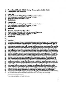
VI. COMPARISON BETWEEN THE CONVENTIONAL AND COGNITIVE APPROACH
To provide a comparison between the conventional and the cognitive approach, the same system of 5 DER units is considered. In the conventional approach, since all DER units share the net power based on the droop characteristic and the assumption that there is no expert dispatcher available for the optimization, the fuel cost is calculated based on the power sharing of individual units. However, in the cognitive approach, the optimization is performed by the CPM, based on the communicated data through CAN. At any optimized efficiency point, the fuel cost is calculated for all DER units and the total cost is calculated for any load conditions. To evaluate the microgird performance, the total fuel cost of all units is used as the final measure. The total fuel cost functions for the given load condition are shown in Figure 20 for both the conventional droop power sharing (red) and the cognitive optimized set points (green). The integral of the fuel cost curve over the given operation period provides the total fuel cost during that period of operation. The shaded area in Figure 20 is proportional to the total fuel cost saving as a result of using the cognitive control strategy.
Off-line and real-time optimizations are introduced in this paper to optimize the fuel-cost of the exportable vehicle power system based smart microgrid. In the conventional approach (non-cognitive), the assumption that there is no expert dispatcher available for the optimization, the fuel cost is calculated based on the power sharing of individual units. However, in the cognitive approach, the optimization is performed by the Cognitive Power Management (CPM), based on the communicated data through CAN. At any optimized efficiency point, the fuel cost is calculated for all DER units and the total cost is calculated for any load conditions. In this approach, some DER units may be disconnected from the microgrid as a result of high operating cost for some load conditions while in the conventional approach all units must be connected to the grid all the time and share their power based on their droop characteristics. The results show that the considerable saving can be achieved in terms of the total fuel cost by using the cognitive control strategy compared to noncognitive approach. VIII. APPENDIX A. Fuel-Cost Curve An approximate Optimum Operating Line (OOL) or optimum efficiency curve for a DER unit can be expressed as a third-order polynomial which is a function of the DER output power [10] 2 3 . (A.1) η = a + b PDER + c PDER + d PDER The Brake Specific Fuel Consumption (BSFC) is given by [11] BSFC (g/kWh) = (Fuel Rate (g/s) × 3600) / Pout (kW).
(A.2)
The output power can be expressed as function of fuel rate and BSFC using (A.2) Pout = Fuel Rare ×3600/ BSFC
(A.3)
The engine input power is also given by [10] Pin = Fuel rate × QHV .
(A.4)
Based on the efficiency definition P η = out . Pin Substituting Pin from (A.4) in (A.5), we have
(A.5)
Fuel Rate = Figure 20. comparison between the conventional and the cognitive approach.
Pout . ηQHV
(A.6)
The cost function is obtained form (A.6) using fuel cost coefficient k ($/kg). C ($/h) = k ($/kg) × Fuel rate (kg/h).
(A.7)
7
Or in a general form, by substituting (A.6) in (A.7) we have
Ci ( PDERi ) =
ki ⋅ PDERi
ηi ⋅ QHVi
,
(E.8)
where Ci is the cost function if ith DER , PDERi is the out put power of ith DER unit, ki is the cost coefficient of ith unit, ηi is the efficiency of the ith unit and, QHVi is the heating value of fuel. B. Study System 1- 5 DER units are considered: a. 1 APU; 408 V; 120 kVA; b. 2 DERs; 408 V; 60 kVA ; c. 2 DERs; 408 V; 30 kVA; 2- All units are connected to the microgrid through %4 impedance with (R/X :1~3); 3- The first unit is operating in voltage mode and the other units (n-1) are in power injection mode; 4- The set points for (n-1) units are provided by CPM based on the off-line optimization;
APU DER1 DER2 DER3 DER4
Load (kW) 20 30 40 50 60 70 80 90 100 110 120 130 140 150 160 170 180 190 200 210 220 230 240 250 260 270 280 290 300
Table B1. DER units data for the fuel cost optimization kW aDERi bDERi cDERi dDERi min max 12 120 0.1303 0.0109 5.8750e-7 −1.5e-4 0 60 0.1303 0.0217 4.7e-6 −0.0006 0 60 0.1503 0.023 5.9e-6 −0.0007 0 30 0.0943 0.0271 2.7765e-5 −0.0016 0 30 0.0253 0.0318 2.8706e-5 −0.0016
ki
QHVLi
0.7 0.9 0.9 1.2 1.3
12 12 12 12 12
Table B2- Optimized dispatch for load steps of 10 kW APU DER1 DER2 DER3 DER4 Total cost (kW) (kW) (kW) (kW) (kW) ($) 20.00 0 0 0 0 3.98 30.00 0 0 0 0 5.17 40.00 0 0 0 0 6.41 50.00 0 0 0 0 7.80 60.00 0 0 0 0 9.43 70.00 0 0 0 0 11.35 60.06 0 19.94 0 0 13.40 55.03 18.22 16.75 0 0 15.86 59.30 21.20 19.51 0 0 17.54 64.03 23.94 22.03 0 0 19.35 69.04 26.55 24.41 0 0 21.32 74.30 29.04 26.66 0 0 23.46 79.84 31.39 28.77 0 0 25.78 85.80 33.54 30.66 0 0 28.29 92.55 35.27 32.18 0 0 30.97 101.93 35.61 32.46 0 0 33.76 120.00 31.31 28.69 0 0 36.03 120.00 36.64 33.36 0 0 38.67 120.00 37.35 33.97 0 8.68 43.77 120.00 41.15 37.09 0 11.76 46.89 120.00 45.40 40.02 0 14.57 50.34 120.00 42.15 37.85 0 30.00 52.14 120.00 48.62 41.38 0 30.00 55.71 120.00 60.00 40.00 0 30.00 58.98 120.00 50.00 60.00 0 30.00 62.37 120.00 49.63 60.00 10.37 30.00 66.67 120.00 60.00 60.00 10.00 30.00 69.94 120.00 60.00 60.00 20.00 30.00 74.80 120.00 60.00 60.00 30.00 30.00 79.47
IX. REFERENCES [1]
F. Katiraei, R. Iravani, N. Hatziargyriou, A. Dimeas, “Microgrids Management”, IEEE Power & Energy Magazine, pp. 54-65, May/June 2008. [2] Driesen, J.; Katiraei, F., “Design for distributed energy resources”, Power and Energy Magazine, IEEE, Volume 6, Issue 3, May-June 2008 Page(s):30 - 40 [3] A.Y. Saber, G.K. Venayagamoorthy, “Intelligent unit commitment with vehicle-to-grid —A cost-emission optimization”, Elsevier, Journal of Power Sources, Vol. 195, Issue 3, pp. 898–911, 2010. [4] W. Shireen, S. Patel, "Plug-in Hybrid Electric vehicles in the smart grid environment," IEEE PES Transmission and Distribution Conference and Exposition, pp.1-4, April 2010. [5] C. Guille, G. Gross, “A conceptual framework for the vehicle-to-grid (V2G) implementation”, Elsevier, Energy Policy, Vol. 37, pp. 4379– 4390, 2009 [6] C. Mi, "Plug-in hybrid electric vehicles - Power electronics, battery management, control, optimization, and V2G", IEEE International Symposium on Industrial Electronics, ISIE 2009. [7] Lopes, J.A.P.; Moreira, C.L.; Madureira, A.G., “Defining control strategies for MicroGrids islanded operation”, Power Systems, IEEE Transactions on, Volume 21, Issue 2, May 2006 Page(s):916 – 924 [8] Katiraei, F.; Iravani, M.R., “Power Management Strategies for a Microgrid With Multiple Distributed Generation Units“, Power Systems, IEEE Transactions on, Volume 21, Issue 4, Nov. 2006 Page(s):1821 – 1831. [9] Leonard L. Grigs, Electric Power Engineering Handbook, Second Edition, CRC Press, 2007. [10] Liu, S.; Stefanopoulou, A.G.; , "Effects of control structure on performance for an automotive powertrain with a continuously variable transmission," Control Systems Technology, IEEE Transactions on , vol.10, no.5, pp. 701- 708, Sep 2002 [11] Modern Electric, Hybrid Electric, and Fuel Cell Vehicles, M. Ehsani and et. al., CRC Press, 2005