ARTICLE International Journal of Advanced Robotic Systems
Local Environment Recognition System Using Modified SURF-Based 3D Panoramic Environment Map for Obstacle Avoidance of a Humanoid Robot Regular Paper
Tae-Koo Kang1, In-Hwan Choi1, Gwi-Tae Park1 and Myo-Taeg Lim1,* 1 School of Electrical Engineering, Korea University, Seoul, Korea * Corresponding author E-mail:
[email protected]
Received 22Aug 2012; Accepted 15Apr 2013 DOI: 10.5772/56552 © 2013 Kanget al.; licensee InTech. This is an open access article distributed under the terms of the Creative Commons Attribution License (http://creativecommons.org/licenses/by/3.0), which permits unrestricted use, distribution, and reproduction in any medium, provided the original work is properly cited.
Abstract This paper addresses a local environment recognition system for obstacle avoidance. In vision systems, obstacles that are located beyond the Field of View (FOV) cannot be detected precisely. To deal with the FOV problem, we propose a 3D Panoramic Environment Map (PEM) using a Modified SURF algorithm (MSURF). Moreover, in order to decide the avoidance direction and motion automatically, we also propose a Complexity Measure (CM) and Fuzzy‐Logic‐based Avoidance Motion Selector (FL‐AMS). The CM is utilized to decide an avoidance direction for obstacles. The avoidance motion is determined using FL‐AMS, which considers environmental conditions such as the size of obstacles and available space. The proposed system is applied to a humanoid robot built by the authors. The results of the experiment show that the proposed method can be effectively applied to a practical environment. Keywords Obstacle Avoidance, 3D Panoramic Environment Map, Avoidance Motion Selection, Complexity Measure, Humanoid Robot www.intechopen.com
1. Introduction The study of humanoid robotics has recently evolved into an active area of research and development. Studies have been published in many related areas of research, such as autonomous walking, obstacle avoidance, stepping over obstacles, and walking up and down slopes and stairs. Yagi and Lumelsky [1] presented a robot that adjusts the length of its steps until it reaches an obstacle, depending on the distance to the closest obstacle in the direction of motion. If the size of the obstacle is small, the robot steps over the obstacle; if it is too tall to step over, the robot starts sidestepping until it clears the obstacle. Obviously, the decision to sidestep left or right is a pre‐programmed one. Kuffner et al. [2] presented a footstep planning algorithm based on game theory that takes into account the global positioning of obstacles in the environment. Chestnutt et al. [3] and Michel et al. [4] presented vision‐ guided foot planning to avoid obstacles using Asimo Honda. These systems get environment information from a top‐down view installed above the humanoid robot.
IntLim: J Adv Robotic Sy, 2013,Recognition Vol. 10, 275:2013 Tae-Koo Kang, In-Hwan Choi, Gwi-Tae Park and Myo-Taeg Local Environment System Using Modified SURF-Based 3D Panoramic Environment Map for bstacle Avoidance of a Humanoid Robot
1
Stasse et al. [5] and Kanehiro et al. [6] presented a stereo‐ vision‐based locomotion planning algorithm that can modify the robot’s waist height and upper body posture according to the size of the available space. Ayaz et al. [7] suggested a footstep approach suited to cluttered environments using a footstep planning algorithm that depends on the obstacle conditions. Gutmann et al. [8] suggested a modular architecture for humanoid robot navigation consisting of perception, control, and planning layers. The existing methods mentioned above use a global path planner that knows all the information on the walking environment. Global path planners, which provide information regarding the walking path and obstacles, have been used to guide humanoid robots to pre‐defined goal positions [3, 8]. However, this assumption that the path planner knows all everything about the walking environment in advance is not appropriate if a humanoid robot walks through an unknown environment. Recently, local environment recognition systems have been studied. Wong et al. have proposed path planning systems using IR‐sensor‐based fuzzy controllers [19] and vision‐based fuzzy controllers [20]. However, these systems do not supply decisions for avoidance direction and the first system does not provide accurate environment information due to the error of the IR sensor. Moreover, the vision‐based fuzzy controller has problems with obstacles beyond the FOV and multi‐ obstacle avoidance. Therefore, in this study, we focus on a local environment system for obstacle avoidance using a 3D‐vision system. In particular, we address the Field of View (FOV) problem. Because the FOV problem occurs whenever humanoid robots meet obstacles that are too large, humanoid robots cannot precisely estimate the obstacle size and decide the appropriate motion. Therefore, we propose a Panoramic Environment Map (PEM) using a Modified Speeded‐Up Robust Feature (MSURF). The conventional SURF [9] has weaknesses with respect to rotation and viewpoint change [10]; therefore, we modified the descriptor of the SURF algorithm by replacing the gradient‐based method with a Modified Discrete Gaussian‐Hermite Moment (MDGHM) method [11]. In [20], the vision‐based fuzzy controller contained a fixed rotation angle according to the avoidance direction, which is inefficient when obstacles are of varying sizes. In this case, the humanoid robot finds it hard to escape various obstacles using only rotation motions with a fixed rotation angle. Therefore, the united avoidance motions of the humanoid robot need to be divided into avoidance direction and avoidance motion in terms of efficiency and adaptability of obstacle avoidance in an unknown walking environment. To achieve this, we propose a Complexity Measure (CM) and Fuzzy‐Logic‐based 2
Int J Adv Robotic Sy, 2013, Vol. 10, 275:2013
Avoidance Motion Selector (FL‐AMS). The CM calculates the complexity of avoidance direction so that a humanoid robot can decide the avoidance direction by itself. The CM values measure the threat to the walking humanoid robot. A high CM value means that the walking environment for the humanoid robot is complex and difficult. As a result, the robot avoids the obstacle by walking in the direction with a lower CM value in terms of efficiency of motion. In addition, we also propose the FL‐AMS method to avoid obstacles using environment information. The fuzzy‐logic‐based control method does not require a mathematical model and has the ability to approximate nonlinear systems. In addition, it can be easily implemented and extended without additional computational cost. In order to specify various motions in the robot, we define the avoidance motion as a combination of two motions based on four basic motions: sidestep walking (S), forward walking (F), rotation walking (R), and turning (T). The FL‐AMS determines the optimal avoidance motion according to the environment information extracted from the PEM. The remainder of this paper is organized as follows. In Section 2, we introduce the local environment recognition system. Section 3 gives the results of experiments to verify the performance of the proposed system. Section 4 concludes the paper by presenting contributions and plans for future work. 2. Local Environment Recognition System Using Modified SURF‐Based 3D Panoramic Environment Map To overcome the FOV problem, we generated a 3D Panoramic Environment Map (PEM) using a MDGHM‐ based SURF algorithm. From the PEM, we can obtain information about obstacles that exist beyond the limited FOV. Then, environment information, such as the location or sizes of obstacles, is extracted. Finally, avoidance motion planning, including avoidance direction and avoidance motion selection, is performed. Detailed methods are presented in the following subsections. 2.1 Architecture of Overall System The overall local environment recognition system architecture is illustrated in Figure 1. The system largely consists of two parts: (1) PEM generation and extraction of environment information, and (2) determination of avoidance direction and avoidance motion. In the first part, we use an MSURF algorithm to generate the PEM. The MSURF algorithm has a modified version of the descriptor stage in the SURF algorithm. In [9], SURF was shown to be sensitive to rotation and viewpoint change caused by the gradient method. Therefore, we modified the conventional SURF using a moment‐based method. The MSURF‐based PEM generation gives environment www.intechopen.com
information more preciseely. To avoid d obstacles in n the on of avoidaance direction n and avoid dance determinatio motion, the robot calcullates the CM M values forr the obstacles exttracted from the PEM and determiness the avoidance diirection. In ad ddition, we prropose FL‐AM MS to select the op ptimal avoidan nce motion in n various wallking environmentts. 2.2 Modified D DGHM‐based S SURF Algorithm 2.2.1 SURF A Algorithm With respect to processing g speed,the SU URF algorithm m is a very efficien nt instrument to accomplish goals succh as searching fo or point corrrespondence between disstinct ness, images. Its p properties, e.g g., repeatabilitty, distinctiven and robustn ness, are stro onger than th hose of previious, similar tools.. The process o of finding poin nt correspond dence between disttinct images iss composed off three main p parts: first, interestt point detectiion, the main component oof the overall proceess; second, feeature vector construction ffrom existing interrest points em mploying inforrmation abou ut the local neighbo ourhood; and third, the ma atching of intterest point pairs by relevant descriptors d frrom each disstinct image [9]. SU URF strictly takes a role in o only two partss: the detector and descriptor paarts.
Modified SURF (MS SURF)
Figu ure 2. Integral Im mage Computattion
PEM gen neration and extraction of enviironment information n) 3D Vision Camera
Disparity Map
PEM Generation
Ano other key com mponent in thee detection sta age of SURF iss the Hessian matrrix that decid des the interesst points, i.e.,, features, require ed. It is maade up of a box filterr app proximation of o a convolu ution result between thee Gau ussian second order partiall derivatives (x‐axis ( and y‐‐ axiss) and the imag ge I . hin a given image, the determ minant of the H Hessian matrix x With also o plays a criticcal role when choosing inte erest points att each h iteration. Th his is perform med through non‐maximum n m supp pression (NMS S) [9]. In additiion, to extract interest pointss from m an image, a G Gaussian approoximation filte er is adapted to o each h level of filter size included iin a scale space e.
The scale space representation r n concept wass also used in n T (Scale‐Invarriant Feature Transform); however, thee SIFT scale space rep presentation u URF is moree used in SU com mputationally efficient and d conserves more high‐‐ freq quency compo onents with n no aliasing. Figure 3 showss the scale space rep presentation oof the SURF allgorithm.
Environment on Information Extractio
Determination of avoidance direction ance motion) and avoida Complexity Measure (CM)
Decision of Avoidance Direction
FL-AMS
Decision of Avoidance Motion
Robot Walking
Figure 1. Geneeration of Panorramic Environm ment Map
2.2.1.1 Detection At the detecttion step, the m major characte eristic of SURF F is a higher speed d than previou us algorithms. In order to ob btain this, the key concept is an n integral ima age adapted too the SURF algoritthm. The inteegral image I (X) is comp puted by the summ mation of all piixels building the input imaage I at position X (x,y)T as
i x j j
I (X X) I(i, j)) (1) i 0 j 0
The processin ng time of thee convolution calculation caan be reduced sharrply using bo ox filtering. Fiigure 2 showss the integral imag ge computatio on. www.intechopen.com
Figu ure 3. Scale space representationn of the SURF a algorithm
As shown in Fig gure 3, by enllarging the siz ze of the box x filteer instead of sccaling down im mages, SURF operates with h bettter speed than n other featuree detectors ussing the moree prev valent concep pt of scale sspace. The fiinal stage off deteecting interesst points is to compute NSM (non‐‐ max ximum suppre ession) over th the neighbourrhood at threee scales. To ensure that one interrest point in th he scale is thee chossen feature, 3 × 3 × 3 n neighbourhoo od pixels aree proccessed, then one o point seleected by NMS S becomes thee keyp point, as show wn in Figure 4..
Tae-Koo Kang, In-Hwan Choi, Gwi-Tae Park and Myo-Taeg Lim: Local Environment Recognition System Using Modified SURF-Based 3D Panoramic Environment Map for bstacle Avoidance of a Humanoid Robot
3
Herrmite polynom mials satisfy th he following orthogonality y cond dition with re espect to the weight functiion exp( x 2 ) as
exp((x
2
In order to assign invarriability to th he interest pooints, every interesst point found d by the dete ector is assign ned a descriptor. W When modificaations happen n to the scene, e.g., viewpoint aangle change,, scale chang ge, blur increease, image rotatio on, image blu ur, compressio on, or illuminaation change, the descriptor of an intere est point can n be employed to identify correspondenc c ces between the original and transformed iimage. In SUR RF, this descrip ption and a is composed of two partss: orientation assignment an Haar wavelet responses‐baased descripto or. In orientatiion assignm ment, image orientation n is specifically u used to make aan interest poiint invariable with respect to im mage rotation n. Orientation n is computed d by detecting thee dominant vector v of the summation s off the Gaussian‐weeighted Haar wavelet ressponses undeer a sliding window circle region spit into regionss in increments o of 3 [9]. To calculatee the descriptor of the in nterest point,, the selected orientation and d the square e region cen ntred around the interest poin nt are needed. In the sq quare 4 split square sub‐ region aboutt the interest point, a 4 × 4 region is asssigned. Thiss acts as the e base stagee for computing tthe horizontal Haar wavellet response, dx , and the verttical Haar waavelet response, dy . Then n the dx and dy from each of o the sub‐reg gions are useed to x, dy, dx , dy ) , calleed a form the vector v=( dx descriptor. S Some restricttions can be e applied to the vector v to m make extended d versions of SURF, i.e., SU URF‐ 36 and SURF F‐128. 2.2.2 Modifiedd DGHM (MDGHM) The DGHM, including th he Hermite po olynomial and d the Gaussian‐Heermite Momen nt (GHM), was w introduceed in [12]. The ptth degree Heermite polyno omial, one off the polynomials, iss given as follo ows: orthogonal p
4
Int J Adv Robotic Sy, 2013, Vol. 10, 275:2013
1
H p (x)
2.2.1.2 Descripption
Hp (x) ( 1)p exp(x2 )
dp dt p
exp( x 2 )
(3))
wheere pq is the Kronecker dellta. In order to obtain the oorthonormal version, thee norm malized Herm mite polynomiaal H p (x) is ca alculated as
Figure 4. Featu ure extraction by y NSM
)Hp (x)Hq (x)dx 2 p p! pq
(2)
2 p p!
exp(
x2 )Hp (x) 2
(4))
Gau ussian‐Hermite functions H p (x / ) can be calculated d by rreplacing x w with x / in (44).
1
H p (x / )
2 p p!
eexp(
x2 2 2
(5))
)H p (x / )
In order o to compute the mom ments for a digital imagee I(i, j) j whose size e is K K [0 i, j K 1] , th he coordinatee tran nsformation over the square [1 x,y 1] iss perfformed using x
2j K 1 2i K 1 (6)) , y K 1 K 1
The Discrete Gaussian‐Her G rmite functio ons can bee equidistance ssampling as a substitute forr calcculated using e the following equ uation. _ 2 1 eexp( x 2 / 2 2 )Hp (x / ) H p (x, ) p K 1 2 p! (7)) _ 1 2 2 H (y, ) 2 e exp( y / 2 )H ) (y / ) q q K 1 2q q! From m (5) and (7)), the DGHM M p,q , which h is a discretee verssion of the GH HM, can be derrived as
p,q
K 1K 1
4 (K K 1)
2
_
_
Hq (y, ) I((i, j)Hp (x, )H i 0 j 0
(8))
The DGHM is a g global feature e representatio on method forr a sq quare image in the discreete domain. Therefore, T wee need d to modify th he convention nal DGHM to represent thee loca al feature of a n non‐square im mage. The Mod dified DGHM M (MD DGHM), proposed by Kangg in [11], is the DGHM of aa massk with sampling intervals . Let I(i, j) be e a digital 2D D image and let t((u,v) be a m mask whose size s is M N The maximum m number off [0 u M 1,0 v N 1] . Th sam mples, k M , k N , are calculateed as follows: k M M / m M , k N N / m N , for t(u,v)
(9))
www.intechopen.com
where m M and m N aare sampling intervals on n the u axis and v axis resp pectively. The pixel values oof the mask t(u,v)((i,j) located at an arbitrary p nput point on the in image I(i, j) aare obtained aas
t(u, v)(i,j) I(u i M 1,v j N 1) (10) 2 2
For orientation assignment, we replace the gradient‐‐ baseed, dx, dy filters based on the Haar wav velet responsee with h MDGHM to o represent thee feature inforrmation moree preccisely. Figure 6 shows an example of the MDGHM‐‐ baseed box filter w whose size is 22s 2s .
For the mask k t(u,v)(i,j) , th he coordinate es are transforrmed such that 1 x,y 1 , as ffollows:
x
2u M 1 2v N 1 (11) , y M 1 N 1
and the Discrrete Gaussian n‐Hermite funcctions of the m mask t(u,v)(i,j) can n be written ass follows:
2 _ H p (x / ) H p (x, ) M 1 2 1 exp( x 2 / 2 2 )H p (x / ) M 1 p 2 p! _ H (y, ) 2 H (y / ) q q N 1 1 2 exp( y 2 / 2 2 )Hq (y / ) N 1 2q q!
Let (ia , ja ) be th he locations oof a keypointt in a digitall e a is the ind dex of the key ypoints. From m image I D , where (13), the MDGHM M‐based box‐fiilter response at (ia , ja ) can n therrefore be calcu ulated as follow ws: (12)
p,q (i, j,mM ,m mN )
4 (M 1)(N 1)
4
kM M 1 k N 1
I D (ia (mM u M 2 1), (14)) p,,q (ia , ja ,m M ,m N ) (M 1)(N 1) u 0 v 0
ja (m N v N 1)))Hp (x, )Hq (y, ). 2
From (10) an nd (12), the MD DGHM with ssampling interrvals at arbitrary p point on the in nput image I(i, j) can be wrritten as follows:
Figu ure 6. Examples of MDGHM‐baased box filter
To extract the dominant dir irection, we calculate thee mag gnitude m(ia , ja ) and angle (ia , ja ) as follows:
m(ia , ja ) ( p,0 (ia , ja )))2 ( 0,q (ia , ja )) )2
k M 1 k N 1
I(i (mMu M 2 1),), (13)
u 0 v 0
j (m Nv N 1))Hp (x, ) Hq (y, ). 2
2.2.3 Modifiedd SURF (MSUR RF) Algorithm In [10], SUR RF was shown n to be sensittive to condittions such as rotattion and view wpoint change es, stemming ffrom the gradient m method used in the descrip ption part of SU URF. To solve th his problem and improv ve the matcching accuracy of tthe SURF algo orithm, we prropose a Mod dified view SURF (MSUR RF) algorithm. Figure 5 presents an overv of the propossed MSURF allgorithm. As shown in n Figure 5, we use MDGH HM for orientaation assignment and descriptiion in conve entional SURF F by calculating an ptor. n MDGHM‐baased orientatio on and descrip
( 0,q (ia , ja )) (ia , ja ) arctan ( (i , j )) p,0 a a
(15))
(16))
The size of the MDGHM‐base M ed box filter is defined ass ows: follo M 2 round(p ) 1, for x‐axiis N 2 round(q ) 1, for y‐axiis
(17))
wheere p and q are the orderrs of the MDG GHM and den notes the stand dard deviation n. All keypoin nts with theirr own n MDGHM‐ba ased magnitud de and orienta ation are used d wheen structurin ng the domiinant orienta ation in thee desccription step of convention nal SURF. Th he rest of thee desccription step of the SURFF descriptor is similar to o conv ventional SUR RF, except thaat we replace e the gradientt mag gnitude and orientation oof the descrip ptor with thee MD DGHM‐based m magnitude and d orientation. 2.3 P PEM generation based on the M F algorithm MSURF‐SURF and extraction of Environment Infformation 1 PEM generation based on thhe MSURF‐SUR RF algorithm 2.3.1
Figure 5. Overrview of MSURF F algorithm www.intechopen.com
As mentioned ab bove, becausee the FOV prroblem occurss wheenever human noid robots m meet obstacless that are too o
Tae-Koo Kang, In-Hwan Choi, Gwi-Tae Park and Myo-Taeg Lim: Local Environment Recognition System Using Modified SURF-Based 3D Panoramic Environment Map for bstacle Avoidance of a Humanoid Robot
5
large, humanoid robots cannot precisely estimatee the priate reaction n. To obstacle’s sizze and decide the approp solve this problem, we w propose the Panor amic M algoriithm. Environmentt Map (PEM)) using the MSURF Table 1 show ws the overalll procedure off PEM generaation. until The procedu ure of PEM geeneration is similar to [13] u the fifth step in Table 1.
the multi‐band blending algorrithm to solve the problem,, whiich blends low w frequencies over a large spatial rangee and d high frequencies over a shoort range [13]..
Figu ure 7 shows an a example off the 3D pano oramic imagess usin ng nine 3D de epth images. FFigure 7(a) sho ows the inputt images gathered ffrom the 3D T TOF camera in nstalled on thee manoid robott and Figuree 7(b) image e shows thee hum resu ulting generate ed 3D panoram mic image.
(a)
Table 1. Algorrithm: Panoramiic Environmentt Map
The first step is to extracct and match h MSURF feattures between two o images. Sin nce MSURF features f are m more invariant to changes in scale, s rotation n, viewpoint, and S our meethod illumination than those off traditional SURF, can handle im mages with vaarying orientation and zoom m. To obtain a goo od solution for the image e geometry att the second stage,, it is only neccessary to sele ect a small num mber of matching pairs to stitcch together a panoramic im mage using the inv variant featurees of overlapp ping images. In n the third stage, w we only consid der the n ima ages that havee the greatest num mber of featuree matches to the current im mage for potential image matchees (we use n 9 ). In this s tage, we use RAN NSAC to select a set off inliers thatt are compatible w with a homog graphy between the imagees. In the fourth sttage, given a set of geome etrically consisstent matches betw ween the imag ges, we use bundle b adjustm ment [13] to provid de solutions ffor all of the camera parameeters jointly. This is an essentiial step, since e concatenatioon of mographies ccauses accumu ulated errors and pairwise hom disregards m multiple constrraints between n images, e.g.,, that the ends of aa panorama sh hould join up. Images are ad dded to the bundlee adjuster one by one, with the best‐matcching image being added at each h step. Then tthe parameterrs are updated usin ng a least squaares frameworrk [13]. h sample (pixeel) along a ray y would havee the Ideally, each same intensiity in every image i that it intersects, bu ut in reality this iss not the case.. Even after ga ain compensaation, some image eedges are stilll visible due to a number off un‐ nsity modelled efffects, such as a vignetting,, where inten decreases tow wards the edg ge of the imag ge, parallax efffects due to un nwanted motion of the e optical ceentre, on errors due to mismodellling of the cam misregistratio mera, radial distorrtion, and so on. Because e of this, a g good blending straategy is imporrtant. In the ffinal stage, wee use 6
Int J Adv Robotic Sy, 2013, Vol. 10, 275:2013
(b) Figu ure 7. The 3D pa anoramic image e generation: (a) nine input imag ges obtained fro om 3D TOF cam mera installed on n the Hum manoid Robot, a and (b) generateed 3D panoramiic image
From m the 3D panoramic p im mage, we can n extract thee obsttacles and theiir informationn. Let and be angles on n the xz and yz planes, respeectively. The key angularr nine 3D TOF im mages in the 3 3D panoramicc posiition for the n image can be esstimated usinng Fast Norm malized Crosss Correlation (FNC CC) [14] as folloows: (u u,v)
v t x,y f(x, y) fu,v t(x u, y v) 2 2 x,y f(x, y) fu,v t(x u, y v)) t
(18))
0.5
wheere f is the 3D D panoramic iimage, t is an n input depth h image from the T TOF sensor, t is the mean o of t , and fu ,v x,y) in the reggion under thee depth imagee is th he mean of f(x E correspo onded point is considered d to have an n t . Each angular position from ‐60 to 600 degrees witth intervals off d The angular posittions for an nd can bee 30 degrees. calcculated from the PEM usiing linear intterpolation ass follo ows: A i ( A i 1 A i ) (x x Ai ) (xx A i1 x A i ), Ai 1 A i 0 A ( A i A i 1 ) (x A x) (xx A x A ), 0 A i 1 A i i i i 1 i (19)) Bi (Bi 1 Bi ) (y yB ) (yyBB yB ), Bi 1 Bi 0 i i 1 i Bi (Bi Bi 1 ) (yBi y) (yBBi y Bi1 ), 0 Bi 1 Bi
wheere A { 60, 30,0,30,60} aand B { 17,,0,17} . Figuree 8 sh hows the results of the 3D P PEM generatiion using (18)) and d (19).
www.intechopen.com
Usin ng (24), the width of tthe obstacless wlk can bee calcculated by ussing the ratioo between th he number off pixeels of the FOV V and the numb mber of pixels o of the obstaclee olk as follows:
Figure 8. Envirronment inform mation result from the PEM imaage
To calculate obstacle inforrmation such a as size or locaation, we need to o transform from spheriical to Carteesian coordinates.
x r sin cos 0 0 y 0 r sin sin 0 z 0 0 r cos
(20)
w lk w FOV (## pok # pFOV ) l
(24))
We can also calcu ulate the anglee kl between n the centre off the robot and the centre of an oobstacle.
lk arctan dxk / dzk l
l
(25))
2.3.2 Extractioon of Environm ment Informatioon In order to eextract the obsstacles, we need to detect b blobs in the 3D PEM. Blob detection is preceded b by a Connected C Component Labelling (CCL L) algorithm [21]. Before blob detection, prreprocessing such as leveel‐set division is carried out beecause CCL operates on biinary images. Let I(xi , y i ,z i ) , i 1, ,N be an PEM a input 3D P with N pixels. The level‐sset is divided d into m bins that affect the in nterval of eaach level‐set. First, we deefine maximum av vailable distan nce d max = 2.5 5 m and m == 50. From the disstance of each pixel zi , leve el‐set is defineed as follows:
I (x k , y k ,z k ) I(x, y,z) k=j y (21) levelsett(I k ) k 0 else
where and k 0, ,m 1 , j floor(floor(z i ) / d) , d d max / m . From the level‐set, obsttacles are ind dexed ollows: by CCL as fo
olk (xlk ,y lk ,zlk ) CCL(I k (x k , y k ,z k ))
(22)
In (22), olk is the l th obsta acle in the kth level‐set extraacted by CCL. Theese indexed obstacles nput o are used u as the in data for deccisions regard ding avoidan nce direction and obstacle anallysis. From (222), we can ca alculate the w width, distance, and d location of th he obstacles. F Figure 9 show ws the parameters u used to calcullate the locatiion and width h for each extracteed obstacle, including i the e angle, size, and distance betw ween obstaclees and the disttance between n the robot and thee obstacle. perpendicularr distance d xk is calculateed as Firstly, the p l follows:
d xk d zk sin FOV (# pco k # pFOV ) l
l
l
(23)
m width of FOV w FOV att the From (23), tthe maximum ulated as follow ws: perpendiculaar distance d xk can be calcu l
w FOV 2 tan( FOV 2) d z k
www.intechopen.com
l
(24)
Figu ure 9. Environme ent information:: location and width calculation
2.4 D Determination of of Avoidance Dirrection and Avooidance Motion 2.4.1 1 Determination of Avoidance e Direction Usin ng the Com mplexity Measure (CM) The environment information n from obstaccle extraction n and d size estimatio on is used as tthe input data a to decide thee bestt direction fo or avoiding obstacles. To o decide thee avoiidance direction, we propoose the comple exity measuree (CM M) as follows: m n k ( 2 lk ) wlk , lk 0 2 2 k 1l 1 m n ( 2lk ) CM C 2k 2 wlk , lk 0 (26)) k 1l1 m n k k k 2 wl , l 0 k 1l 1 As sshown in (26), the CM is deetermined by three factors:: the distance between the robbot and the obstacle, thee wid dth and the height of the obbstacle, and th he angle of thee obsttacle from the robot’s curreent direction. T The CM has aa larg ge value in cases c where the robot is close to thee obsttacle, where the angle from m the centre of o the PEM to o
Tae-Koo Kang, In-Hwan Choi, Gwi-Tae Park and Myo-Taeg Lim: Local Environment Recognition System Using Modified SURF-Based 3D Panoramic Environment Map for bstacle Avoidance of a Humanoid Robot
7
the obstacle is small, and where the obstacle is large in size. A large CM value indicates that the environment is too complex for the robot to avoid the obstacle. Therefore, we get the final avoidance decision from the determination value D as follows:
D sign(
D 0, turn right (27) CM) D 0, turn left all obstacle
In (27), the CMs for obstacles located on the left side of the robot have negative values, and the CMs for obstacles located on the right side of the robot have positive values. Therefore, the avoidance direction can be determined by the summation of all CMs over all obstacles. If D is positive, the robot turns to the left, and if D is negative, the robot turns to the right. 2.4.2 Decision of Avoidance Motion Using a Fuzzy‐Logic‐ Based Avoidance Motion Selector (FL‐AMS)
T(w i ) {A1 ,A 2 ,A 3 ,A 4 ,A 5 } {NL,NS,Z,PS,PL}
T(si ) {B1 , B2 , B3 , B4 , B5 } {NL,NS,Z,PS,PL}
T(fi ) {C1 ,C 2 ,C 3 ,C 4 ,C 5 ,C6 ,C7 } {ST,SS,SF,RS,RF,TS,TF}
Int J Adv Robotic Sy, 2013, Vol. 10, 275:2013
Rule R(j1 , j2 ) :
(30)
IF w i is A j and di is B j2 , then fi is Cf( j
1 ,j2 )
1
j1 {1,2,3,4,5}, j2 {1,2,3,4,5}, f(j1 , j2 ) {1,2,3,4,5,6,7}
1
0.75
NS
0.5
(27) (28)
Z PS PL
0.25
0 10
20
30
40
50
60
70
80
90 100 110
wi
(a)
1
0.75 NL NS 0.5
Z PS PL
0.25
0 0
15
30
45
60
75
90
105
120
si
(b)
1
0.75
TF TS
(29)
where fuzzy sets A1 ,A 2 ,A 3 ,A 4 , and A 5 are respectively denoted as Negative Large (NL), Negative Small (NS), Zero (Z), Positive Small (PS), and Positive Large (PL) for the input variable w i . Fuzzy sets B1 , B2 , B3 , B4 , and B5 are also respectively denoted as Negative Large (NL), Negative Small (NS), Zero (Z), Positive Small (PS), and Positive Large (PL) for the input variable di . Fuzzy sets 8
NL
After choosing the direction to take to avoid the obstacle, a motion type must be selected based on the environment conditions. To achieve this purpose, we need an intelligent control approach. Fuzzy logic is one such approach that does not require mathematical modelling and has the ability to approximate nonlinear systems. In addition, it can be easily implemented and extended without additional computational cost. Therefore, we propose a fuzzy‐logic‐based avoidance motion selector (FL‐AMS). In order to perform fuzzification [15], the difference w i between the obstacle width and robot width and the space difference Si between the avoidance space width and the robot width are set up as the input variables. Figure 10 shows the input and output membership functions. As shown in Figure 10, triangular‐type membership functions and fuzzy‐singleton‐type membership functions are used for the input and output variables, respectively. The term sets of the input and output variables are selected as follows:
C1 ,C 2 ,C 3 ,C 4 ,C 5 ,C6 , and C7 are respectively denoted as Stop (ST), Slip step + Slip step (SS), Slip step + Forward step (SF), Rotation step + Slip step (RS), Rotation step + Forward step (RF), Turning step + Slip step (TS), and Turning step + Forward step (TF). All of these are combinations of any two motions: Slip step (S), Forward step (F), Rotation step (R), Turning step (T), but excluding the Stop motion (ST) for the output variable fi .
RF 0.5
RS SF SS
0.25
ST
0 1
2
3
4
5
6
7
fi
(c) Figure 10. Membership functions of fuzzy system: (a) Input variable w i , (b) input variable s i , and (c) output variable fi www.intechopen.com
Table 2. Fuzzy y rule table for F FL‐AMS
To determinee the final outtput of the FL L‐AMS, we usee the weighted aveerage method described by:: j1 5 j2 5
u j1
fi f ( wi , si )
j1 1 j2 1
j2 v C f
j1 j2
(31)
j1 5 j2 5
u j1 j2
j1 1 j2 1
where v(Cf(( j ,j ) ) is the crisp value of the fuzzy y set, 1 2 Cf( j ,j ) . The function u(j1 , j2 ) is the fire strength off the 1 2 rule R(j1 , j2 ) and can be deescribed by:
u(j1 , j2 ) m min( A (w i ), B (si )) (32) j1
j2
he width diffference w i between obsstacle Based on th width and ro obot width an nd space diffe erence s i betw ween avoidance sspace width and robot width, w the s even values fi , i {1,2,3,4,5,6,7 evaluation v 7} for the s even avoidance motions can be determined by the FL‐AMSS. nsist of seven Walking mottion types con n motions, SSS, SF, RS, RF, TS, aand TF, which h are combinattions of two oof the motions sid destep walkin ng (S), forwa ard walking (F), rotation walk king (R), and turning (T), e excluding the stop motion (ST). Table 2 show ws the fuzzy rule table forr the walking motiions.
Figu ure 11. Humanoid Robot Designn and GUI
The height of the humanoid roobot is about 6 600 mm. Each h joint is driven by the RC servoomotor, which h consists of aa DC motor, gear, and simple controller. Our humanoid d robo ot also has 23 2 degrees of f freedom (DOF) and two o diffeerent vision sy ystems, a 3D T TOF camera an nd a webcam.. As shown s in Figure 11, the G GUI largely co onsists of fourr partts: the 3D VR R image, the webcam ima age, the TOF F cam mera image, an nd the 3D PEM M. The design ned humanoid d robo ot system has two vision syystems: a webcam and a 3D D TOF F camera, which are shown on the webca am image partt and d TOF camera image part off the GUI, resp pectively. Thee 3D PEM image part p shows thee PEM genera ated by using g the MSURF algo orithm. Finallyy, the 3D VR R image part,, imp plemented using the OpenG GL library [18], shows thee anallysed environ nmental inform mation. Table e 3 shows thee speccifications of o our humanoid d robot system m.
3. Experimenttal Results for IIntelligent Obsstacle Avoidan nce
Type
We carried d out expeeriments to investigate the effectiveness of local enviironment reco ognition using g the proposed M MSURF algoriithm. Our ex xperiment larrgely consists of acccuracy testin ng for environ nment informaation and the succcess rate off obstacle av voidance for the designed hum manoid robot.. A detailed description of tthese is presented b below.
Heigght : 600 mm AT991SAM7s256 (AR RM7 core)
Actuator (RC S Servo motors)
RC SServo motors (RX‐‐28 * 3, RX‐64 * 8, RX‐106 * 12) 23 D DOF (Leg + Arm A + Head +
Degree of Freedom
Waist)) = 2*66 + 2*4 + 2 + 1
3.1 Humanoidd Robot Design
www.intechopen.com
Size CPU
Power Sourc ce
For this expeeriment, we designed d and built a humaanoid robot. The ov verall constru uction of our h humanoid rob bot is shown in Fig gure 11.
Specification
Sensors
Pow wer supply (17 V V) 3D: T TOF camera (SR R‐4000) 2D: W Webcam
Tablle 3. Specificatio on of the designned humanoid rrobot
Tae-Koo Kang, In-Hwan Choi, Gwi-Tae Park and Myo-Taeg Lim: Local Environment Recognition System Using Modified SURF-Based 3D Panoramic Environment Map for bstacle Avoidance of a Humanoid Robot
9
3.2 Experimen ntal Setup We implemeented our obsttacle avoidancce approach u using the humano oid robot witth a TOF cam mera. The viision system on th he robot’s heead provides disparity im mages (176 × 144) aat 30fps. For testing t our pe erception metthod, we set up an n obstacle env vironment con ntaining obstaacles and avoidancce spaces of diifferent sizes.
Figure 12. Exp periment environ nment
As shown in n Figure 12, th he experiment space was 22.5 m × 3 m and tthere were tw wo types of artificial a obstaacles which had d dimensions of 32 cm (W) × 32 cm (H) × 24 cm (D). These were used in variious combina ations so thatt we could make o obstacles of diifferent widths and spacing g. We evaluated fou ur related alg gorithms: a SIF FT‐based metthod, a PCA‐SIFT‐‐based metho od, a conventiional SURF‐b based method, and d the propossed MSURF‐b based method d, as tabulated in Table 4. We set the MSU URF parameterrs to p q 3 , 0.3 , m M m N 1 and ussed a window w size of 5s 5s . Feature Extraction n Orientation n Assignmen nt Descriptorr
SURF[16] MSURF SIFT [13] Hessian
Hessian
PCA A‐ SIFT[[17]
DoG
Tablle 5. Experimen ntal results for siize estimation u using four SUR RF‐related algoriithms
Table 5 shows th he results for ssize estimatio on for variouss distances and sizes using the four SURF‐related d algo orithms.In Ta able 5, the rresults for the estimated d h of obstacle distance, the esttimated width es, and PEM M geneeration times were averaged d over 20 trialls. As sshown in Tablle 5, although the generatio on time for thee MSU URF‐based method is a litttle slower tha an the SURF‐‐ baseed method, th he MSURF‐baased method shows betterr perfformance than the others with respecct to the sizee estim mation of the obstacles.Figu ure 13 shows ssome examplee PEM M images usin ng the MSURF algorithm.
(a)
DoG G
Haar MDGHM Grradient Gradiient Wavelet Haar MDGHM Hisstogram PCA A Wavelet
(b)
Table 4. Charaacteristics of fou ur SURF‐related algorithms testted
3.3 Experimen nt Results for E Environment Infformation To estimate obstacle inforrmation, we proposed p the P PEM image using g the MDGH HM‐SURF allgorithm. In this section, we tested the accuracy a of the obstacle size estimation o of the proposeed method and compared d the results with those of thee PEM image e using the SIFT algorithm. In n this experim ment, we tested d the perform mance of size estimation for fourr types of obsttacles with wiidths of 71.3 cm, 95.4 cm, 119.5 cm, and 142.8 vely, 8 cm, respectiv 20 times for eeach width. 10 Int J Adv Robotic Sy, 2013, Vol. 10, 275:2013
(c)
(d)
Figu ure 13. Example PEM images m made using MSU URF for an obstacle at 105 cm d distance: widthss of obstacle are (a) 71.3 cm, (b) 9 95.4 cm, (c) 119.5 5 cm, and (d) 1442.8 cm www.intechopen.com
3.4 Experimen nt Results for D Decisions of Avooidance Directio ion and Avoidancee Motion We tested our proposed method under varrious anoid robot was environmentaal conditions. The huma programmed to walk and d stop when it i met an obsstacle d or defined diistance. Then th he humanoid rrobot within a fixed determined th he decision faactors needed to avoid obstaacles. We carried ou ut the experim ments regardin ng the decision n and control perforrmance under various obstaccle conditions. ormance of the e FL‐AMS meethod First, we veriified the perfo proposed in this paper fo or walking obstacle avoid dance manoid robott. In Table 6, a a confusion m matrix using the hum shows that tthe proposed algorithm confidently pre dicts the correct m motion decisiion. In Table 6, one thoussand random valu ues consisting g of the obstacle size and d the avoidance sp pace were used as the input, and the outtputs are tabulated d for each situaation.
Table 6. Confu usion matrix forr motion decisio ons
Seco ondly, we testted the decisioon and controll performancee und der various obstacle condiitions: obstaclle width and d avoiidance space. The experimentall results are sh hown in Table e 7, Figure 14,, and d Figure 15. We W tested the oobstacle avoid dance walk off the humanoid rob bot under eacch condition 50 times. If thee hum manoid robot a arrived at the destination w we defined forr it, th he walking te est succeeded.. On the other hand, if thee hum manoid robot collided witth an obstacle or got lostt duriing walking, it failed. A As shown in Table 7, thee prop posed method d has a high su uccess rate eve en without an n optiimal control method for walking. To improve thee succcess rate of a humanoid roobot system, a a vision‐based d ptive walking adap g control sysstem is neede ed for futuree worrk.
(a)
As shown in n Table 6, the FL‐AMS sho ows good deciision accuracies, 98% (980/10000) for SS motion, 998.7% (987/1000) for SF motion, 998.4% (984/100 00) for RS mootion, 99.1% (991/1000) for RF motion, m 98.8% (988/1000) foor TS motion, 99.44% (994/ 10000) for TF motion, and 9 9.5% (995/1000) forr ST motion.
(b)
Figu ure 14. Experime ental Results unnder various obsstacle cond ditions: (a) SS m motion type, (b) SSF motion type
Figu ure 14 illustra ates a resultiing image sequence when n usin ng SS and SF m motion types,, and Figure 1 15 presents an n image sequence that resulted d when using g RS and RF F mottion types. In tthe cases show wn in Figures 14 and 15, thee resu ults show goo od avoidance e performance e because thee wid dths of the obsstacles are reaasonable for the t humanoid d robo ot.
Table 7. Experrimental results for obstacle avo oidance www.intechopen.com
Tae-Koo Kang, In-Hwan Choi, Gwi-Tae Park and Myo-Taeg Lim: Local Environment Recognition System Using Modified SURF-Based 3D Panoramic Environment Map for bstacle Avoidance of a Humanoid Robot
11
5. R References
(a)
(b)
Figure 15. Exp perimental Results under variou us obstacle conditions: (a) RS motion typee, (b) RF motion n type
4. Conclusion n In this paper, we introduced the lo ocal environm ment recognition system using g an MSURF F‐based PEM M for obstacle avoiidance of a humanoid h rob bot. The prop posed method is b based on a PEM image using an M MSIFT PEM algorithm, v vision‐based CM, C and FL L‐AMS. The P image metho od can be a so olution for ove ercoming the FOV problem, wh hich may bee a major ca ause of incoorrect decisions in n walking control and d perception n of environmentt. The vision‐b based CM sy ystem decide es the avoid dance direction forr a humanoid d robot to av void obstaclees by considering environment informatio on such as the distribution of obstacles, distance from the humaanoid robot to the o obstacles, and size of each o obstacle. Finally, the FL‐AMS systtem automatiically decidess the best avoidaance motion depending on the obsstacle conditions u using the enviironment info ormation obtaained by the PEM. These system ms do not ne eed a global path planner with h all inform mation regard ding the obsstacle location and d path inform mation in ad dvance. From m the experimentall results, wee believe tha at our prop posed methods willl be useful for humanoiid robots in real environmentts.
12 Int J Adv Robotic Sy, 2013, Vol. 10, 275:2013
[1] Yagi Y M, Lume elsky V (19999) Biped Robo ot Locomotion n in Scenes wiith Unknown n Obstacles. Proceedings off IEEE International Confference on Robotics R and d Automation (ICRA). pp. 3775‐380. [2] Kuffner JJ, Ni K ishiwaki K, Kaagami S, Inab ba M, Inoue H H (2001) Footstep Planning A Among Obstacles for Biped d Robots. Pro oceedings off IEEE/RSJ Internationall Conference on Intelligen ent Robots and a Systemss (IROS). pp. 500‐505. [3] Chestnutt C J, Lau L M, Cheun ng G, Kuffner J, Hodgins J,, Kanade T (2 2005) Footstep p Planning fo or the Hondaa ASIMO Hum manoid. Proceeedings of th he 2005 IEEE E Internationall Conferencce on Ro obotics and d Automation. pp. 629‐ 634. [4] Michel M P, Ch hestnutt J, Ku uffner J, Kan nade T (2005)) Vision‐guided Humanoid d Footstep Planning forr Dynamic Env vironments. P Proceedings off the 5th IEEE‐‐ RAS Internattional Confereence on Huma anoid Robots.. pp. 13‐18. [5] Stasse O, Verr S relst B, Vanderrborght B, Yok koi K (Augustt 2009) Strattegies for Humanoid Robots to o Dynamically Walk Overr Large Obsstacles. IEEE E Transactions on Robotics. 225: 4: 960‐967. [6] Kanehiro F, Yo K oshimi T, Kajitta S, Morisaw wa M, Fujiwaraa K, Harada K,, Kaneko K, H Hirukawa H, To omita F (Aprill 2005) Whole Body Locomootion Planning of Humanoid d Robots based d on a 3‐D Gri rid Map. Proce eedings of thee 2005 IEEE In nternational C Conference on Robotics and d Automation. pp. 1072‐ 10788. [7] Ayaz Y, Konn A o A, Munawaar K, Tsujita T,, Uchiyama M M (2009) Plann ning Footstep ps in Obstaccle Cluttered d Environmentts. Proceedin ngs of the IEEE/ASME E Internationall Conference on Advance ed Intelligentt Mechatronicss. pp. 156‐161.. [8] Gutmann G JS,, Fukuchi M M, Fujita M M (2008) 3‐D D Perception and a Environm ment Map Generation forr Humanoid Robot R Navigaation. Internattional Journall of Robotics R Research. 27: 1 0: 1117‐1134. [9] Bay B H, Tuyte elaars T, Goool LV (2008) Speeded Up p Robust Featu ures (SURF). C Computer Vision and Imagee Understandin ng. 110: 346‐3559. [10] Juan L, Gwu un O (2009) A Comparison of SIFT, PCA‐‐ SIFT, and SURF. S Internaational Journ nal of Imagee Processing. 3 3: 4: 143‐152. Z H, Kiim DW, Parrk GT (2012)) [11] Kang TK, Zhang Enhanced SIFT S Descrip ptor Based on o Modified d Discrete Gau ussian‐Hermitte Moment. ETRI E Journal.. 34: 4: 572‐582 2. [12] Yang B, Dai M (2011) Imaage Analysis by Gaussian‐‐ Hermite Moments. Signall Processing. 91: 10: 2290‐‐ 2303. owe D (2007) A Automatic Pan noramic Imagee [13] Brown M, Lo Stitching ussing Invarian nt Features. Internationall Journal of Co omputer Vision n. 74: 1: 59‐73.
www.intechopen.com
[14] Zhang K, Lu J, Lafruit G, Lauwereins R, Gool LV (2009) Robust Stereo Matching with Fast Normalized Cross‐Correlation Over Shape‐Adaptive Regions. Proceedings of the 16th IEEE International Conference on Image Processing. pp. 2357‐2360. [15] Mendel JM (2001) Uncertain Rule‐Based Fuzzy Logic Systems: Introduction and New Directions, Prentice‐ Hall. [16] Juan L, Gwun O (2010) SURF Applied in Panorama Image Stitching. Proceedings of Image Processing Theory, Tools, and Applications. pp. 495‐499. [17] Ke Y, Sukthankar R (2004) PCA‐SIFT: A More Distinctive Representation for Local Image Descriptors. Proceedings of the International
[18] [19]
[20]
[21]
Conference on Computer Vision and Pattern Recognition. pp. II‐506‐513. http://www.opengl.org/ Wong C, Cheng C, Huang K, Yang Y (2008) Fuzzy Control of Humanoid Robot for Obstacle Avoidance. International Journal of Fuzzy Systems. 10: 1: 1‐10. Wong C, Hwang C, Huang K, Hu Y, Cheng C (2011) Design and Implementation of Vision‐Based Fuzzy Obstacle Avoidance Method on Humanoid Robot. International Journal of Fuzzy Systems. 13: 1: 45‐54. Shapiro L, Stockman G (2002) Computer Vision. Prentice Hall.
www.intechopen.com
Tae-Koo Kang, In-Hwan Choi, Gwi-Tae Park and Myo-Taeg Lim: Local Environment Recognition System Using Modified SURF-Based 3D Panoramic Environment Map for bstacle Avoidance of a Humanoid Robot
13