Local hidden--variable models for entangled quantum states

arXiv:1405.7321v1 [quant-ph] 28 May 2014

Local hidden–variable models for entangled quantum states R Augusiak1 , M Demianowicz1 , and A Ac´ın1,2 1

ICFO–Institut de Ciencies Fotoniques, Mediterranean Technology Park, 08860 Castelldefels (Barcelona), Spain 2 ICREA–Institucio Catalana de Recerca i Estudis Avan¸ cats, Lluis Companys 23, 08010 Barcelona, Spain Abstract. While entanglement and violation of Bell inequalities were initially thought to be equivalent quantum phenomena, we now have different examples of entangled states whose correlations can be described by local hidden–variable models and, therefore, do not violate any Bell inequality. We provide an up to date overview of the existing local hidden–variable models for entangled quantum states, both in the bipartite and multipartite case, and discuss some of the most relevant open questions in this context. Our review covers twenty five years of this line of research since the seminal work by Werner [R. F. Werner, Phys. Rev. A 40, 8 (1989)] providing the first example of an entangled state with a local model, which in turn appeared twenty five years after the seminal work by Bell [J. S. Bell, Physics 1, 195 (1964)], about the impossibility of recovering the predictions of quantum mechanics using a local hidden–variables theory.

CONTENTS

2

Contents 1 Introduction

2

2 Preliminaries and notation 2.1 Entanglement . . . . . . . . . . . . . . . . . . . . . . . . . . . . . . . . 2.2 Measurement in quantum theory . . . . . . . . . . . . . . . . . . . . . 2.3 Bell-type experiment and local models . . . . . . . . . . . . . . . . . .

3 3 3 5

3 Bipartite quantum states 3.1 Werner’s model . . . . . . . . . . . . . . . . . . . . . . . . . . . . . . . 3.2 Barrett’s model for the Werner states . . . . . . . . . . . . . . . . . . 3.3 Nonlocality of noisy states: the Grothendieck constant . . . . . . . . . 3.4 Noise robustness of correlations: Almeida et al. ’s model . . . . . . . . 3.5 From projective to generalized measurements — Hirsch et al. ’s construction . . . . . . . . . . . . . . . . . . . . . . . . . . . . . . . . .

9 10 14 17 22

4 Multipartite quantum states 4.1 Local model for projective measurements on GME tripartite states . . 4.2 Generalizations and discussion . . . . . . . . . . . . . . . . . . . . . .

29 29 31

5 Other locality scenarios

32

6 Conclusions and outlook

33

Appendix A

35

27

1. Introduction In 1935, the concepts of local–hidden variable model and entanglement were introduced in the works by, respectively, Einstein, Podolsky and Rosen [1], and Schr¨ odinger [2]. After them, very few works (see, e.g., [3, 4]) considered the problem of whether local models may provide a more intuitive, and complete, alternative to the quantum formalism until 1964, when Bell showed that local models are in fact in contradiction with quantum predictions. In particular, he proved that local models satisfy some inequalities, known thereafter as Bell inequalities, that are violated by the statistics of local measurements on a singlet state [5]. The work of Bell started the study of quantum nonlocality, that is, of those correlations obtained when performing local measurements on entangled states that do not have a classical analogue. Initially, it was believed that entanglement and quantum nonlocality were equivalent phenomena. And, in fact, entanglement and nonlocality do coincide for pure states, as any pure entangled state violates a Bell inequality [6]. However, in 1989 Werner introduced a family of highly symmetric mixed entangled states, known today as the Werner states, and exploited the symmetries of these states to construct an explicit local model reproducing the correlations for some of them [7]. The work by Werner then implied that the relation between nonlocality and entanglement is subtler than expected and, in particular, these two notions do not coincide in the standard scenario originally introduced by Bell. After Werner’s work, several other results have appeared providing new local models for other entangled states. The main purpose of this article is to review all these

CONTENTS

3

existing models. Our hope is that this review will be useful to have a broad vision of what is known today on the relation between entanglement and quantum nonlocality, in particular in the case when an entangled state satisfies all Bell inequalities. As it will become clear below, the explicit construction of local models has turned out to be an extremely difficult problem and, at the moment, we only have a few models beyond Werner’s original construction. In fact, in our view, most, if not all of the existing models, can be interpreted, in a way or another, as variants of Werner’s model. The structure of the review is the following: after introducing the main concepts and definitions used in our work, we go through all the existing models, both in the bipartite and multipartite scenario. We then briefly discuss other possible definitions of nonlocality, such as, for instance, the concept of hidden nonlocality introduced by Popescu [8]. Finally, we present our conclusions and a list of open questions. 2. Preliminaries and notation We start by introducing notions and definitions repeatedly used throughout the manuscript: entanglement and genuine multipartite entanglement, measurement in quantum theory, and the Bell–experiment setup with the corresponding notions of locality. In what follows by B(H), 1d , Ωd , and ωd we denote, respectively, the set of bounded linear operators acting on a finite-dimensional Hilbert space, the d×d identity matrix, the set Ωd = {|λi ∈ Cd |hλ|λi = 1}, and the unique distribution over Ωd invariant under any unitary operation U acting on Cd . 2.1. Entanglement Let us consider two parties, traditionally called Alice (A) and Bob (B), sharing a bipartite quantum state ρAB acting on a product Hilbert space H = CdA ⊗ CdB . We say that ρAB is separable iff it can be written as a convex combination of pure product states [7], that is X X i i ρAB = pi |ψA ihψA | ⊗ |φiB ihφiB |, pi ≥ 0, pi = 1 (1) i i |ψA i

dA

i

|φiB i

dB

with some ∈ C and ∈ C . Otherwise, it is called entangled. In a general multiparty scenario with N parties we will denote them A(1) , . . . , A(N ) =: A. Let Ak be a k element subset of A and Ak its complement in the said set. Then, an N partite state ρA is said to be biseparable if it can be written as X X ρA = pAk |Ak ρAk |Ak , pAk |Ak = 1, (2) Ak |Ak

Ak |Ak

where each ρAk |Ak is separable (see (1)) across the bipartition Ak |Ak and the sum goes over all such bipartitions. If a state cannot be written as (2) it is called genuinely multiparty entangled (GME). 2.2. Measurement in quantum theory d We call a collection {Pa }k−1 a=0 of k projections acting on C a k-outcome projective measurement (PM; also called von Neumann measurement) if the Pa are supported

CONTENTS

4

on orthogonal subspaces, i.e., Pa Pa0 = Pa δaa0 , and k−1 X Pa = 1 d ,

(3)

a=0

where by 1d we denote the d × d identity operator. With a projective measurement Pk−1 with outcomes αa , a = 0, 1, · · · , k − 1, we associate an operator A = a=0 αa Pa called an observable which is measured in the measurement process. In what follows, we just talk about performing measurement A. Performed on a state %, a measurement will give the ath outcome αa corresponding to Pa with the probability p(a|A) given by the Born rule p(a|A) = tr(Pa %). The mean value of an observable in the state % is given by k−1 X hAi := tr(A%) = αa p(a|A).

(4)

(5)

a=0

Clearly, when d = 2 a projective measurement can have only two outcomes represented by rank-one projections Pa (of course, there is also a trivial single-outcome projective measurement with P0 = 1d , which we do not need to consider here). In general, however, the projectors Pa do not necessarily have to be rank one, and, in fact, if k < d there must exist at least one of rank larger than one. d A collection of k operators A = {Aa }k−1 a=0 acting on C is called a k-outcome POVM, where POVM stands for Positive-Operator Valued Measure, or k-outcome generalized measurement if they are positive, i.e., Aa ≥ 0, and k−1 X Aa = 1d . (6) a=0

The latter, in particular, means that every Aa is upper bounded by the identity, i.e., Aa ≤ 1d . The probability of obtaining the outcome a corresponding to Aa is given again by the Born rule, that is, by Eq. (4) with Pa replaced by Aa . In what follows the operators Pa forming a projective measurement as well as Aa forming a generalized measurement will be called measurement operators. Obviously, every projective measurement is also a POVM, the opposite, however, is in general not true. Equivalently speaking, for a given dimension d, the set of all projective measurements forms a proper subset of all generalized measurements †. It is important to note, however, that whenever we deal with d outcome measurements on Cd they are necessarily projective. For further benefits, we also notice that in our considerations we can in fact assume that measurement operators, both in the case of projective and generalized measurements, are rank-one, or, in other words, the measurements are nondegenerate. This is because any measurement whose operators are of rank larger than one can always be realized as a measurement with rank-one operators. More precisely, since every element Aa of a generalized measurement is a positive operator P (a) (a) (a) (a) it admits the form Aa = i ηi Pi with 0 ≤ ηi ≤ 1 and Pi being, respectively, the eigenvalues and the rank-one eigenprojectors of Aa . Moreover, due to Eq. (6), all the eigenvalues must satisfy X (a) ηi = d. (7) i,a

†The restriction to the fixed dimensions is very important here since any POVM can be realized formally as a PM in a larger space.

CONTENTS

5 (a)

(a)

Now, denoting all these new rank-one operators as Aa,i = ηi Pi it is clear that they also form a POVM which is a “finer grained” version of {Aa }. To reproduce the statistics of the “coarse grained” original POVM, one simply applies the finer POVM {Aa,i } and forgets the result i. In this way, a local model (see the upcoming section for the relevant notion) for POVMs with rank-one measurement operators will imply a local model for any POVM. It is also worth mentioning that whenever we work with qubits it is beneficial to exploit the Bloch representation of quantum states and projection operations. A state ρ acting on C2 can be expressed as 1 (8) ρ = (12 + ρ · σ) 2 with ρ ∈ R3 being the so-called Bloch vector of length kρk ≤ 1 and σ = (σx , σy , σz ) standing for a vector consisting of the standard Pauli matrices‡. Bloch vectors of unit length correspond to rank-one projectors. Within the Bloch representation the measurement operators Pa associated to a generalized measurement (see the discussion above) are represented by the Bloch vectors pa which due to (6) must satisfy k−1 X

ηa pa = 0.

(9)

a=0

In particular, if k = 2 the projections Pa form a a projective measurement and the above condition simplifies to p0 + p1 = 0.

(10)

This implies that any two-outcome measurement defined on a qubit Hilbert space is fully represented by a single vector, say p ≡ p0 . Also, in the case of two-outcome projective measurements we will mainly use the more standard notation for the outcomes denoting them ±1 instead of 0, 1. Then, in the Bloch representation the projectors corresponding to the outcomes can be represented as 1 P± = (12 ± p · σ) (11) 2 and the mean value of an observable A is just hAi = p(1|A) − p(−1|A). 2.3. Bell-type experiment and local models Let us now consider N spatially separated parties A(1) , . . . , A(N ) = A sharing some N -partite quantum state ρA acting on a product Hilbert space H = Cd1 ⊗ . . . ⊗ CdN with di < ∞ (i = 1, . . . , N ) denoting the local dimensions. On their share of ρA , (i) each party is allowed to perform one of m (possibly generalized) measurements Axi (xi = 1, . . . , m), each with d outcomes, which we enumerate as ai = 0, 1, . . . , d − 1. We usually refer to such a scenario as to (N, m, d) scenario (of course, one can consider a more general case of different number of measurements and outcomes at each site, but such a scenario is a straightforward generalization of the present one). In the case of small number of parties N = 2, 3 we will rather denote them by A, B, C, and the corresponding measurements and outcomes by A, B, C and a, b, c, respectively.  ‡The Pauli matrices are defined as: σx =

0 1

1 0

  0 , σy = i

−i 0



 , σz =

1 0

0 −1

 .

CONTENTS

6

The correlations generated in such an experiment are described by a set of probabilities (N ) p(a1 , . . . , aN |x1 , . . . , xN ) := p(a1 , . . . , aN |A(1) x1 , . . . , AxN )  i h (N ) ρA = tr A(1) x1 ⊗ · · · ⊗ AxN (1)

(12)

(N )

of obtaining results a1 , . . . , aN upon measuring Ax1 , . . . , AxN . In what follows, the set (12) will also be referred to as quantum correlations or, simply, correlations. Also, it is useful to think of the set {p(a1 , . . . , aN |x1 , . . . , xN )}, after some ordering, as of a vector from RD with D = dN mN . Actually, by using the nonsignalling constraints (see, e.g., [9,10]) one finds that a significantly lower number D0 = [m(d−1)+1]N −1 of probabilities is sufficient to fully describe the correlations (12). For further purposes let us finally notice that in the case d = 2, one can equivalently describe the correlations by a collection of expectation values (ik ) 1) hA(i xi1 . . . Axi i

(13)

k

with xi1 , . . . , xik = 1, . . . , m, i1 < . . . < ik = 1, . . . , N , and k = 1, . . . , N . Here (i ) Axikk are dichotomic observables with outcomes ±1. There are precisely [m + 1]N − 1 of such expectation values, which matches the number of independent probabilities D0 in this scenario. This equivalence does not hold if d > 2 simply because the number of independent probabilities exceeds that of correlators (13) (see, nevertheless, Refs. [11, 12] for possible ways to overcome this problem). It is known that the set of quantum correlations, denoted QN,m,d , that can be produced in the above experiment from all states and measurements is convex (provided one does not constrain the dimension of the underlying Hilbert space). A proper subset QN,m,d is formed by those correlations that the parties can obtain by using local strategies and, as the only resource, some shared classical information, often called shared randomness, λ, distributed among them with probability distribution ω(λ). Mathematically, this is equivalent to saying that each probability (12) can be expressed as Z (N ) (N ) p(a1 , . . . , aN |A(1) , . . . , A ) = dλ ω(λ)p(a1 |A(1) (14) x1 xN x1 , λ) · . . . · p(aN |AxN , λ) Ω

with Ω denoting the set over which the random variable λ is distributed and (i) p(ai |Axi , λ) are local probability distributions conditioned additionally on λ. It follows that in any scenario (N, m, d), the set of local correlations, i.e., those admitting the representation (14), is a polytope PN,m,d whose vertices are the local deterministic correlations of the form (N ) (1) (N ) p(a1 , . . . , aN |A(1) x1 , . . . , AxN ) = p(a1 |Ax1 ) · . . . · p(aN |AxN ) (i)

(15)

with the local probabilities being deterministic, that is, p(ai |Axi ) ∈ {0, 1} for all outcomes and settings. In passing, let us notice that as PN,m,d has a finite number of vertices, the integration in (14) can always be replaced by a finite sum over these vertices; for further purposes it is however easier for us to use the integral representation. As already mentioned, QN,m,d is strictly larger than PN,m,d and quantum correlations that fall outside PN,m,d are named nonlocal. Natural tools to witness nonlocality in correlations are the so–called Bell inequalities [5] (see also [13] and references therein for examples thereof). These are linear inequalities that constrain

CONTENTS

7

the set of local correlations and their violation is a signature of nonlocality (see Fig. 1). For a given scenario (N, m, d), Bell inequalities can be most generally written as β :=

d−1 X

m X

,...,aN p(a1 , . . . , aN |x1 , . . . , xN ) ≤ βL , (16) Txa11,...,x N

a1 ,...,aN =0 x1 ,...,xN =1

where T is some tensor whose entries can always be taken nonnegative and βL is the so-called classical bound of the inequality and is given by βL = maxPN,m,d β (clearly, here it suffices to maximize only over the vertices of PN,m,d in order to determine βL ). An illustrative example of a Bell inequality in the simplest (2, 2, 2) scenario is the famous Clauser-Horne-Shimony-Holt (CHSH) Bell inequality [14]: 1 2 X X

p(a ⊕ b = (x − 1)(y − 1)|xy) ≤ 3,

(17)

a,b=0 x,y=1

which can be restated in terms of the expectation values (13) as |hA1 B1 i + hA1 B2 i + hA2 B1 i − hA2 B2 i| ≤ 2.

(18)

Here Ai and Bi (i = 1, 2) are pairs of dichotomic observables with eigenvalue ±1 measured by the parties A and B, respectively. It is known that in the (2, 2, 2) scenario the CHSH inequality (18) is the only “relevant” Bell inequality as it defines all facets of P2,2,2 [15]. In other words, if a bipartite state ρAB does not violate the inequality (18) for any choice of the measurements Ai and Bi , then it does not violate any other Bell inequality in this scenario. The CHSH inequality is an example of a correlation Bell inequality, in which only the joint terms hAi Bj i appear. A schematic depiction of all the above concepts is provided in Fig. 1. quantum correlations local deterministic correlations polytope of local correlations

Bell inequality

nonlocal correlations Figure 1. Quantum and local correlations. Local correlations form a polytope (blue gray region), denoted N,m,d , with vertices being the local deterministic correlations of the form (15) (blue points). This set forms a proper subset of the set of quantum correlations, N,m,d , given by (12) (orange region). Correlations falling outside N,m,d are called nonlocal (red point) and can always be detected with the help of a Bell inequality. On the scheme we give two examples of such inequalities (thick lines), the one corresponding to the facet of the polytope (on the right) is called tight, and, accordingly, the other is said to be not tight.

P

P Q

Now, within this framework, we call the state ρ local in the scenario (N, m, d) if the probability distribution that can be generated from it is local for any choice

CONTENTS

8 (i)

of the measurements Axi with xi = 1, . . . , m and i = 1, . . . , N . Notice that if ρ is local in the scenario (N, m, d), then it is local in any scenario (N, m0 , d0 ) with either m0 < m or d0 < d. On the other hand, there are states that are local in some scenario (N, m, d), but their nonlocality can be revealed only when the number of measurements or outcomes is increased. Finally, a state ρ is called local if it is local in a scenario with any number of measurement and outcomes. Equivalently, one says that ρ has a local-hidden variable (LHV) model or simply a local model. Notice that in such case, one can drop all the subscripts xi in (14) because any probability generated from ρ must take such a form. As a result, (14) simplifies to Z p(a1 , . . . , aN |A(1) , . . . , A(N ) ) = dλ ω(λ)p(a1 |A(1) , λ) · . . . · p(aN |A(N ) , λ). (19) Ω

On the other hand, if there is a scenario (N, m, d) in which for some choice of measurements the resulting probability distribution (12) does not admit the form (14), we call ρ nonlocal. Of course, one can further distinguish the case when ρ is local only under projective measurements, i.e., (14) holds if the measurements A(i) with i = 1, . . . , N are projective. Then, one says that ρ has a local model for projective measurements. Moreover, for d = 2, one can also formulate the definition of locality of quantum states in terms of expectation values (13). Then, every expectation value involving more than two parties admits the form (19) with local probabilities replaced by the corresponding one-body mean values “conditioned” on λ. Notice furthermore that a model reproducing global probability distribution automatically reproduces local statistics as the latter are just the marginals of the former. The situation is more subtle when we work with the expectation values (13). Here, a local model realizing expectation values involving some number of parties, say k, does not necessarily properly describes expectation values involving less than k parties. In particular, in the bipartite case, a model reproducing joint expectation values hABi may not reproduce hAi and hBi; we refer to such model as to a model for joint correlations. This observation will be of particular importance in Sec. 3.3. From the point of view of the resources shared by the parties, the question of whether a state has a local model is the question of whether shared classical randomness can replace it in the described setup (see Fig. 2). It is clear that an unentangled state is trivially local in any scenario as the global probability of local measurements is a sum of factorized components. In the remainder of this paper we thus focus on providing LHV models for entangled states and genuinely multipartite entangled state in the multipartite case (cf. Sec. 4). In the most general setting such a model simulating statistics of the measurements A and B with the results a and b, respectively, will be given as follows (for brevity we give a bipartite version): General local model (0) Alice and Bob are distributed some classical information λ belonging to some Ω with probability distribution ω(λ), (1) Alice outputs a according to some probability distribution p(a|A, λ) conditioned on A and λ, (2) and, likewise, Bob outputs b according to the probability distribution p(b|B, λ).

CONTENTS

9

Figure 2. Simulating quantum probabilities with classical information. A schematic illustration of the concept of locality of quantum states. For simplicity we consider the bipartite case. Imagine that the parties A and B perform a pair of measurements A and B on some bipartite (entangled) state ρAB obtaining results a and b, respectively. Locality of ρAB means that the resulting probability distribution p(a, b|A, B) for any pair A, B can also be obtained if the parties shared some classical information represented by λ instead of ρAB . Phrasing differently, one can simulate statistics arising from local quantum states by using purely classical resources.

In the above, p(a|A, λ) and p(b|B, λ), also called response functions, determine the strategies parties need to employ to simulate measurements on a given quantum state (it is not difficult to see that without loss of generality they could be taken deterministic [15]). Once these mappings are proposed it will be the main task to verify whether (19) holds with l.h.s. arising from measurements on a quantum state of interest. Notice that in the general model we stated, the nature of λ is not an issue. It can be a single variable (discrete or continuous), a set of variables, etc. Also the case of Alice and Bob receiving different λs is covered in this very general formulation. 3. Bipartite quantum states We start our tour through local models with bipartite scenarios. In such setting the first and most famous model is due to Werner [7] who already in 1989 realized that projective measurements on some entangled states give rise to local statistics. These states belong to the class which is usually referred to as the Werner states. Besides presenting the original model we will also discuss several of its modifications. Many years later the result by Werner was generalized by Barrett [16] who proved that local models may account for statistics even of generalized measurements on some entangled Werner states. The price one had to pay for such extension was the diminishment of

CONTENTS

10

the region of parameters of the applicability of the model. At this moment, it is not known whether Werner states are local for projective and generalized measurements in the same region of the parameter. An important line of research in the domain has been the analysis of the nonlocal properties of noisy states, i.e., the ones which arise as the mixture of some state with the white (completely depolarized) noise. This problem was addressed by Ac´ın et al. [17] and Almeida et al. [18]. In the former work, nonlocal properties of such states were related to the Grothendieck constant [19], establishing, in particular, the region in which two-qubit Werner state is local for projective measurement. In the latter, building on the previous works by Werner and Barrett about local models and the protocol by Nielsen for the deterministic conversion between pure entangled states by local operations and classical communication (LOCC) [20], values of the critical noise thresholds for locality of noisy states were obtained. We will conclude this section with a recent result by Hirsch et al. [21] who found a method of constructing states with local models for POVMs from states with local models only for two outcome projective measurements. 3.1. Werner’s model The class of states considered by Werner consists of all two-qudit states that are invariant under a bilateral action of any unitary operation, i.e., they commute with U ⊗ U for any unitary U acting on Cd . Such states are of the form 2Pd 1d + (1 − p) 2 d(d − 1) d   d−1+p 1 = 1d − pVd , d(d − 1) d (−)

ρW (d, p) = p

(−)

(20)

(+)

where Pd (Pd ) stands for the projector onto the antisymmetric (symmetric) subspace of Cd ⊗ Cd and Vd denotes the so-called swap operator defined through Vd |φ1 i|φ2 i = |φ2 i|φ1 i

(21)

for any pair |φ1 i, |φ2 i ∈ Cd . It is useful to recall that = (1d ± Vd )/2. Also, when (−) d = 2, P2 = |ψ− ihψ− | is just the projection onto the two-qubit singlet state √ |ψ− i = 1/ 2(|01i − |10i). (22) (±) Pd

It was shown in Ref. [7] that Werner states ρW (d, p) are separable if and only if p ≤ pW,c sep with 1 . (23) d+1 In particular, it is very easy to see that they are entangled for any p > 1(d + 1) as the swap operator Vd is also an entanglement witness [22, 23] detecting them, i.e., Tr[ρW (d, p)Vd ] < 0 in this region. Let us now show, following Ref. [7], that for any p ≤ pW,c PM with pW,c sep ≡

pW,c PM ≡

d−1 d

(24)

CONTENTS

11

these states always give rise to local statistics when measured with projective measurements. In fact, it is enough to show this for the boundary value of the mixing parameter p = pW,c PM , for which Eq. (20) reduces to  
1 d+1 d d−1 1d − V d . (25) ρW d, d = 2 d d For all values of p < pW,c PM the result will follow immediately because one can always obtain the corresponding ρW (d, p) by mixing ρW (d, pW,c PM ) with some portion of the white noise 1d /d2 which itself clearly admits a local model and the state given by the mixture of states with local models has also a local model. Now, it directly stems from Eq. (25) that the quantum” probability of obtaining outcomes a and b when performing the von Neumann measurements A and B represented by projections {Pa } and {Qb }, respectively, amounts to   1 d+1 W − Tr(Pa Qb ) , (26) pQ (a, b|A, B) = 2 d d where we have used the well-known property of the swap operator that Tr(Vd X ⊗Y ) = Tr(XY ) for any pair of matrices X, Y. To simulate (26) with local strategies Werner proposed the following model: LHV model for projective measurements on Werner states (Werner’s model) [7] (0) Alice and Bob are distributed shared randomness represented by a one-qudit pure state |λi ∈ Cd (the hidden state space is Ωd = {|λi ∈ Cd | hλ|λi = 1}) with the unique distribution invariant under any unitary operation ωd (λ), (1) Alice returns the outcome a for which the overlap hλ|Pa |λi is the smallest one, i.e., her response function reads ( 1, if hλ|Pa |λi = minhλ|Pα |λi α p(a|A, λ) = , (27) 0, otherwise (2) Bob returns the outcome b with probability p(b|B, λ) = hλ|Qb |λi.

(28)

For further purposes it is worth noting that the response functions (27) and (28) have the following equivariance property p(a|A, U λ) = p(a|U AU † , λ),

p(b|B, U λ) = p(b|U BU † , λ)

(29)

for any unitary U acting on C . Let us mention in passing that originally in Ref. [7] both the response functions were exchanged. This, however, does not affect the final result as the Werner states are permutationally invariant. The latter also means that we can even symmetrize the roles of the parties in the protocol. This can be easily done by augmenting the protocol with an additional two–valued hidden variable determining which type of the function, (27) or (28), each of the party must choose as the response. Having all the necessary ingredients, we can now demonstrate that indeed pW (a, b|A, B) admits the form (19) with N = 2, i.e., Q Z W pQ (a, b|A, B) = dλ ωd (λ)p(a|A, λ)p(b|B, λ). (30) d

Ωd

CONTENTS

12

To be more instructive and explanatory, we will exploit for this purpose the approach of Ref. [24] rather than the original one by Werner. We start by noting that the value of the integral in (30) is, by the very construction of the model, invariant under any unitary rotation applied to |λi. This means that we can decompose |λi in the eigenbasis {|ii} of Alice’s observable A, i.e., X |λi = λi |ii (31) i

with λi being some complex coefficients such that |λ1 |2 +. . .+|λd |2 = 1. In what follows we will exploit their polar representation, that is, λi = ri exp(iφi ) with 0 ≤ ri ≤ 1 and φi ∈ [0, 2π) for any i. Clearly, r12 + . . . + rd2 = 1. Additionally, without any loss of generality, we can assume that the projection corresponding to the particular outcome a appearing in (30) is simply Pa = |1ih1|. All this allows us to rewrite the probabilities (27) and (28) as ( 1, r12 = min rα2 α=2,...,d p(a|A, λ) = (32) 0, otherwise and p(b|B, λ) =

d X

hi|Qb |jiri rj ei(φj −φi )

i,j=1

=

d X

d X hi|Qb |jiri rj ei(φj −φi )

hi|Qb |iiri2 +

i=1

(33)

i6=j

respectively. Inserting these into (30) and performing integrations over all the angles φi (clearly, the second summand in the above formula gives zero), one arrives at Z d 1 X hi|Qb |iiJ(ui ), (34) dλ ωd (λ)p(a|A, λ)p(b|B, λ) = N i=1 Ωd with the functional Z J(h) =

1

Z

1

du1 0

Z

1

dud h(u1 , . . . , ud )δ(u1 + . . . + ud − 1),

du2 . . . u1

u1

(35) ri2

where we have made the substitution = ui . The Dirac delta in the above is due to the normalization of |λi, while the lower bounds in the integrations over u2 , . . . , ud follow from the condition in (32). Finally, Z 1 Z 1 N= du1 . . . dud δ(u1 + . . . + ud − 1). (36) 0

0

One can significantly simplify the computation of the right-hand side of (34) by noting that the integrals in (35) are manifestly symmetric under any permutation of the variables u2 , . . . , ud (but not u1 !) and therefore J(u2 ) = . . . = J(ud ). Moreover, the delta function in (35) allows us to conclude that J(u2 )+. . .+J(ud ) = J(1)−J(u1 ), which in turn means that J(ui ) = [J(1) − J(u1 )]/(d − 1) for any i = 2, . . . , d. Putting pieces together, we have that Z [d Tr(Pa Qb ) − 1]J(u1 ) + [1 − Tr(Pa Qb )]J(1) , (37) dλ ωd (λ)p(a|A, λ)p(b|B, λ) = N (d − 1) Ωd

CONTENTS

13

where we have substituted back Pa for |1ih1|, which in particular means that h1|Qb |1i is now Tr(Pa Qb ), and we have also used the fact that Tr Qb = 1 for any b. To complete the proof, one then needs to determine the values of the integrals J(1) and J(u1 ). Computation of the latter has been done in Appendix A and its value has been found to be J(u1 ) = N/d3 .

(38)

The value of J(1) can be inferred directly from the above formula (37): exploiting the fact that p(a|A, λ) and p(b|B, λ) are proper probability distributions, by summing both its sides over a and b, one obtains that J(1) = N/d. Inserting both integrals into the right-hand side of Eq. (37), one finally obtains the quantum probability (26). As a result, the above model allows one to show that the probabilities arising from projective measurements performed on the subsystems of the Werner states can always be simulated by a local model for any p ≤ (d−1)/d. Since the boundary value (d−1)/d is larger than the separability threshold 1/(d+1) of ρW (d, p), this means that for any d there are entangled states with local model for projective measurements. Noticeably, the critical value grows with d, while the one for separability drops, meaning that the models becomes more powerful for larger d (cf. Fig. 3). Remark 1. Let us also notice that the above model, initially designed for two-outcome projective measurements at each site, works also if a generalized measurement with any number of outcomes is allowed at Bob’s site. This directly follows from the facts that Bob’s response function is linear in the measurement operators and that the measurement operators of a POVM B can be taken as Bb = ξb Qb with rank-one operators Qb and some positive constants ξb (see Sec. 2.2). Therefore the probabilities realized by the model in this case are pL (a, b|A, B) = ξb pL (a, b|A, B 0 ), where pL (a, b|A, B 0 ) denote unnormalized “probabilities” obtained by measuring projectors Qb on Bob’s site. At the same time, one realizes that the quantum probabilities are pQ (a, b|A, B) = ξb pQ (a, b|A, B 0 ), and therefore pL (a, b|A, B) = pQ (a, b|A, B). Remark 2. Interestingly, as shown by Gisin and Gisin in Ref. [25], one can simulate the statistics of the singlet state (or, equivalently, the Werner state for p = 1) with a local model if Alice or Bob (or both) are allowed not to provide outcomes. To state the model we now switch, for simplicity, to the Bloch representation, however, all that follows can be restated in terms of vectors from Cd . Assume that Alice and Bob receive unit vectors a and b representing local projective measurements A and B, respectively, and a unit vector λ from the Bloch sphere generated according to the uniform distribution ω e (λ) = 1/4π. Now, Alice follows the same strategy as in Werner’s model, that is, she always outputs −sgn(a · λ) with sgn denoting the sign function. Then, with probability |b · λ|, Bob accepts λ and outputs sgn(b · λ) in this case, while if he does not accept λ, he does not give any outcome. The local expectation values hAi = hBi = 0, while the correlation produced by this model taken over all the “accepted” λ are given by Z 1 dλ|b · λ|sgn(a · λ)sgn(b · λ) hA ⊗ Bi = − 2π Z 1 = − dλ sgn(a · λ) (b · λ) 2π = − a · b, (39)

CONTENTS

14

where to obtain the last equation we have followed the calculation from Appendix A. The corresponding probabilities are given by 1 (a, b = ±1) (40) p(a, b|A, B) = (1 − ab a · b) 4 and they agree with (26) for d = 2. Looking at Eq. (39), one can realize that this model can also be understood as one with a distribution (1/2π)|b · λ| which depends on the measurement of Bob. In other words, a model with a distribution that depends on the measurements of one of the parties can reproduce even highly nonlocal correlations. In fact, this observation was used in [26] to construct models for the simulation of entangled states using classical communication or supra-quantum resources. Remark 3. Building on the above result, one can introduce a local model reproducing statistics obtained on a two-qubit state that differs from the two-qubit Werner state [21]. Alice follows the same strategy as above, while Bob whenever he does not accept λ, outputs b = ±1 with probability (1 ± hη|b · σ|ηi)/2. After some calculation one finds that the class of states whose correlations are simulated by this model is given by ρ = p|ψ− ihψ− | + (1 − p)

12 2

⊗ |ηihη|.

(41)

with p ≤ 1/2. Remark 4. Let us conclude by noting that one can also extend the applicability of Werner’s model by playing with the distribution ω. An example of a distribution different than the uniform one has been recently given in [27] and reads ω(λ) = (1 + λ3 )/4π, where λ3 is the third coordinate of the Bloch vector λ. In such case, the model corresponds to the two-qubit state   1−p 12 12 ρ(p) = p|ψ− ihψ− | + 2|0ih0| ⊗ +3 ⊗ |1ih1| (42) 5 2 2 with p ≤ 1/2. Notice that this state is a convex combination of two states given in Eq. (41). 3.2. Barrett’s model for the Werner states Let us now present the local model for general measurements for the Werner states due to Barrett [16]. Now, Alice and Bob want to simulate the probability distribution arising from some generalized measurements, A and B, with the measurement operators Aa = ηa Pa and Bb = ξb Qb (cf. Sec. 2.2) performed on Werner states (20). One quickly finds that this distribution is not much different from that for projective measurements (26) and simply reads   ηa ξb d−1+p W pQ (a, b|A, B) = − p Tr(Pa Qb ) . (43) d(d − 1) d The model now goes as follows: LHV model for POVMs on Werner states (Barrett’s model) [7] (0) As in Werner’s model, the set of hidden states and the distribution are, respectively, Ωd and ωd ,

CONTENTS

15

(1) Alice returns the outcome a according to the response function: p(a|A, λ) = hλ|Aa |λiΘ(hλ|Pa |λi − 1/d) ! X ηa + 1− hλ|Aα |λiΘ(hλ|Pa |λi − 1/d) , 2 α

(44)

(2) Bob returns the outcome b with the probability p(b|B, λ) =

ξb (1 − hλ|Qb |λi). d−1

(45)

In the above, Θ is the Heaviside step function, i.e., Θ(x) = 1 for any x ≥ 0 and Θ(x) = 0 for x < 0. To demonstrate that the above model recovers (43) and also to determine the range of p for which this is the case, let us insert the response functions (44) and (45) into (30). After some algebra, this leads us to 1 ξb X η a ξb − Jab + Jaβ pW L (a, b|A, B) = 2 d d−1 d−1 β

+

ηa d(d − 1)

X α

Jαb −

ηa ξb X Jαβ d(d − 1)

(46)

αβ

with Z dλ ωd (λ)Θ(hλ|Pa |λi − 1/d)hλ|Pa |λihλ|Qb |λi.

Jab = ηa ξb

(47)

Ωd

In order to perform the above integration, let us decompose |λi as in (31) with λi = ri exp(iφi ) and the basis {|ii} chosen so that it contains a vector corresponding to Pa (recall that now the projectors Pa as well as Qb do not have to be orthogonal). As previously, we can assume that Pa = |1ih1|. With this parametrization, one finds that (47) becomes now Jab =

d ηa ξb X e 1 uk ], hλ|Qb |λiJ[u N

(48)

k=1

e is defined where the normalization factor N is given by (36), while the functional J[h] as Z 1 Z 1 Z 1 e = J[h] du1 du2 . . . dud h(u1 , . . . , ud ) δ(u1 + . . . + ud − 1). 1/d

0

0

(49) e 1 u2 ] = . . . = J[u e 1 ud ], one easily sees that J[u e 1 uk ] = {J[u e 1] − By noting that J[u 2 e J[u1 ]}/(d − 1), which allows one to further simplify (48) to o ηa ξb n e 21 ] + [1 − Tr(Pa Qb )]J[u e 1] . [d Tr(Pa Qb ) − 1]J[u Jab = N (d − 1) (50) After inserting this into (46), one arrives at the following expression ( ) e 2 ] − J[u e 1]  1 dJ[u 1 1 W pL (a, b|A, B) = ηa ξb + − Tr(Pa Qb ) , (51) d2 N (d − 1)2 d

CONTENTS

16

which, when compared with (43), shows that the above model reproduces joint probabilities for the Werner states for any p ≤ pW,c POVM with the critical probability given by pW,c POVM = d

e 2 ] − J[u e 1] dJ[u 1 . N (d − 1)

(52)

To finally determine the explicit value of pW,c POVM one has to compute the integrals e 1 ) and J(u e 2 ). This can be done by exploiting basically the same approach as in J(u 1 the case of projective measurements (the detailed calculations are moved to Appendix A), which leads us to   d−1 d−1 e 1 ] = N 2d − 1 (53) J[u d d d and e 2] = N J[u 1 d2



5d − 3 d+1



d−1 d

d−1 ,

(54)

and in consequence pW,c POVM =

3d − 1 d(d + 1)



d−1 d

d−1 .

(55)

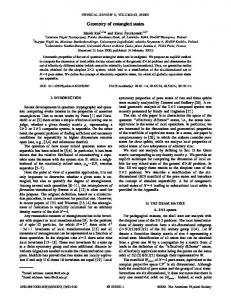
W,c Interestingly, pW,c POVM > psep for any d, and as a result Barrett’s model reproduces statistics of generalized measurements for entangled Werner states for any d. However, unlike in Werner’s model, pW,c POVM is a (monotonically) decreasing function of d. Moreover, it decreases faster than pW,c sep , meaning that the range of p for which this W,c , p ], shrinks with d → ∞. Fig. 3 compares the three is the case, i.e., p ∈ (pW,c sep POVM W,c W,c W,c critical values psep , pPM , and pPOVM for various values of the local dimension d.

mixing parameter p

1.0 0.8

ò

ò ò ò ò ò ò ò ò ò ò ò ò ò ò ò ò

ò

0.6 ò

0.4 0.2 0.0

à æ

à æ à æ à æ æ à à à æ æ æ à æ à æ à æ à æ à æ à æ à æ à æ à æ à æ à æ à

5

10 15 dimension d

20

Figure 3. Critical probabilities for the Werner states. Comparison of three critical values of the probabilites for the Werner states for 2 ≤ d ≤ 20: pW,c sep W,c W,c (green dots), pW,c POVM (red squares), pPM (green triangles). Noticeably, while psep decays with d, the critical value pW,c PM grows, implying that for large d almost all the entangled Werner states are simulable by local models.

Remark 5. As noticed by Barrett [16], a bipartite state ρ ∈ B(CdA ⊗ CdB ) that has a local model for generalized measurements induces a whole family of states with local models (some of which might naturally be separable). The construction goes

CONTENTS

17

as follows: let Ω, ω(λ), p1A (a|A, λ) and p1B (b|B, λ) denote, respectively, the space of local variables, the distribution and the response functions in the local model for ρ for general measurements A = {Aa } and B = {Bb }. Consider then two (in general 0 different) quantum channels§ ΛX : B(CdX ) → B(CdX ), X = A, B, and the state obtained from ρ through σ = (ΛA ⊗ ΛB )(ρ).

(56)

Now, σ has a local model for generalized measurements with the same hidden state space Ω, distribution ω and response functions defined as p2A (a|A, λ) = p1A (a|A0 , λ),

p2B (b|B, λ) = p1B (b|B 0 , λ) 0

(57) 0

with the measurements operators of the generalized measurements A and B given by A0a = Λ†A (Aa ),

Bb0 = Λ†B (Bb ),

(58)

†

where Λ is a dual¶ map of Λ. As a dual map of a quantum channel is positive and unital (it preserves the identity operator), the operators A0a and Bb0 form proper quantum measurements. To see eventually that the functions (57) do define a local model for σ it is enough to apply the following argument Z dλ ω(λ)p2A (a|A, λ)p2B (b|B, λ) = Tr(A0a ⊗ Bb0 ρ) Ω

= Tr[Λ†A (Aa ) ⊗ Λ†B (Bb )ρ] = Tr[Aa ⊗ Bb (ΛA ⊗ ΛB )(ρ)] = Tr[Aa ⊗ Bb σ],

(59)

where to pass from the second to the third line we have exploited the definition of the dual map to Λ. Let us conclude by noting that the above argument can also be applied to the multipartite states, provided such states with local models for generalized measurements exist. Actually, it applies to any state that has a “mixed” local model, i.e., one which works for projective measurements at some sites and for generalized measurements at the rest. In such case, to obtain a new state local quantum channels discussed above can be applied only to those sites. An example of such a state and the corresponding “mixed” local model will be discussed in Section 4.1. 3.3. Nonlocality of noisy states: the Grothendieck constant We now move to the analysis of nonlocal properties of noisy quantum states, that is states of the form

1

, ρ ∈ B(Cd ⊗ Cd ). (60) d2 As mentioned at the beginning of this section, this problem can be related to the mathematical constant KG known as Grothendieck constant [19]. The connection between the latter and nonlocality was first recognized in 1987 by Tsirelson (a.k.a. Cirel’son) [28] who considered the problem of how large is the set of quantum correlations compared to the set of classical ones. The interest in this surprising ρ(d, p) = pρ + (1 − p)

§Recall that a linear map Λ : B(H) → B(K) with H and K being two finite-dimensional Hilbert spaces is called a quantum channel iff it is completely positive and trace-preserving. ¶A dual map to a linear map Λ : B(H) → B(K) is a linear map Λ† : B(K) → B(H) that satisfies Tr[XΛ(Y )] = Tr[Λ† (X)Y ] for all X ∈ B(K) and Y ∈ B(H).

CONTENTS

18

relationship had its revival almost thirty years later when it was analyzed in greater detail by Ac´ın et al. in Ref. [17]. The results of the latter paper, relevant for our review, may be summarized as follows (the terminology and necessary definitions will be introduced in what follows): h1i projective measurements on a two–qubit Werner state, ρW (2, p) (see Eq. (20)), can be simulated with an LHV model if and only if p ≤ 1/KG (3), h2i local models for ρW (2, p) exist in the whole√range where the state does not violate CHSH inequality (17), that is for p ≤ 1/ 2, when at least one of the parties is restricted to perform planar measurements, h3i whenever p ≤ 1/KG (2d2 ) there is a local model reproducing joint correlations of traceless two-outcome observables for the state (60) with any ρ. Moreover, for p > 1/KG (2blog2 dc + 1) there exists ρ(d, p) without such a model. In particular, in the limit of d → ∞ both bounds match and every noisy state is local below 1/KG and this number cannot be made larger. Before we proceed, we need the definition of the Grothendieck constant. Let n ≥ 2 be integer, M be an arbitrary m × m real matrix such that for all real numbers a1 , a2 , · · · , am , b1 , b2 , · · · , bm from the interval [−1, +1], it holds X m Mij ai bj ≤ 1. (61) i,j=1 The Grothendieck constant of order n, KG (n), is defined to be the smallest number such that X m Mij ai · bj ≤ KG (n), (62) i,j=1 for all unit vectors ak , bk ∈ Rn The Grothendieck constant, KG , is then defined through KG = lim KG (n). n→∞

(63)

It is quite remarkable that such constant even exists; it is also interesting that the √ exact values of the constants, besides KG (2) = 1/ 2 [29], are not known. The bounds for the constants appearing in our analysis are as follows [29–32]: 1.6770 ≤ KG ≤ 1.7822,

(64)

KG (8) ≤ 1.6641,

(65)

1.417 . KG (3) ≤

π , 2c3

where c3 is the unique, in the interval [0, π/2], solution of the equation Z c3 √ c3 dx x−3/2 sin x = 2.

(66)

(67)

0

Numerically one then finds that KG (3) ≤ 1.5163. Let us now elaborate on each of the items h1i-h3i from the list above.

(68)

CONTENTS

19

As to the point h1i, let us first notice that the reconstruction of mean values hA ⊗Bi, hAi, and hBi is enough to retrieve full probability distribution as we deal here with two-outcome measurements in which case the number of mean values matches the number of independent probabilities necessary for this task (see the discussion in Section 2). Further, on states with maximally mixed reductions (for two qubits these are the Bell diagonal states), including the discussed Werner state ρW (2, p), local expectation values vanish, hAi = hBi = 0. The key point of the analysis now is that given a model reproducing correctly only hA ⊗ Bi, we can turn it into one for which also local mean values vanish: we augment the old protocol with an extra random bit and in the new model parties just multiply outputs of the old one by the value of this bit ensuring that joint prediction are still the same and local ones are vanishing. Thus, nonlocal properties of ρW (2, p) are uniquely determined by the joint correlations solely and in the following analysis we can restrict ourselves to correlation Bell inequalities. The latter in the most general case can be written as X m Mij hAi ⊗ Bj i ≤ βL , Mij ∈ R, (69) i,j=1 where βL denotes the local bound of a given Bell inequality, that is X m Mij ai bj βL = max ai ,bj =±1 i,j=1

(70)

since deterministic strategies are sufficient to achieve it. Clearly, we can normalize our inequality such that βL = 1 and we will assume this has been done. Now, correlations on the maximally mixed state vanish and thus violation of any correlation Bell inequality by Werner states is determined by its violation by the singlet state. Since for the latter we have hAi ⊗ Bj iψ− = ai · bj , this violation maximized over all Bell inequalities can be written just as m X Mij ai · bj . (71) βQ,W := lim sup max m→∞ Mij ai ,bj i,j=1 From this it immediately follows that no Werner state ρW (p, 2) can violate a correlation Bell inequality in the range p ≤ 1/βQ,W . As one can easily see, βQ,W is just the Grothendieck constant KG (3), and so we have recovered that whenever p ≤ 1/KG (3) a two-qubit Werner state is local for projective measurements and no local model can exist for values outside this range. Taking into account (68) we realize that this result is an improvement over Werner’s p ≤ 1/2, as√1/KG (3) ≥ 0.6595. It is known that there is a gap between the exact value and 1/ 2 ' 0.7071 as the Werner state have been demonstrated to violate some Bell inequality for p > 0.7056 [31] (cf. Fig. 4). Recall that ρW (2, p) is entangled when p > 1/3. As announced in h2i, there is no such separation when (at least) one of the parties is restricted to perform measurements on a plane in the Bloch sphere. In this case vectors ai are two dimensional, moreover, bj can be taken to lie in the same plane since only the scalar products of a and b are contributing to the value of the Bell operator. In this way√it is clear that the bound now involves KG (2), which, as mentioned, is equal to 1/ 2. The result, which is an improvement over 2/π from [33], then follows. The statement of h3i is a result of the attempt to generalize h1i to arbitrary dimensions. However, we encounter two difficulties in such generalization. First, we

CONTENTS

20

need to restrict ourselves to two-outcomes measurements (for the reason discussed in Section 2). Second, even in this case we cannot hope to give full characterization of nonlocal properties of a state with the aid of the correlation Bell inequalities only. This stems from the fact that in the general approach we pursue here we cannot assume that our states are locally maximally mixed and thus it might be necessary to use inequalities with local terms [34] for this purpose. Thus, we can only hope here to fully characterize the joint correlations. Further, an additional requirement will have to be met: tracelessness of the observables. This condition ensures that the averages on the maximally mixed state are zero and the Grothendieck constant approach can be employed. To proceed it might be useful to rephrase h3i using the critical probability pc (d) for states of the form Eq. (60). For a given d, this is a minimum over all states ρ of the maximal p for which there exists a local model in the given scenario. With this notion in hand, the claims are that 1 1 ≤ pc (d) ≤ (72) KG (2d2 ) KG (2blog2 dc + 1) and 1 pc (∞) := lim pc (d) = . (73) d→∞ KG We start with the left-hand side of (72) and consider first states ρ(i) (d, p) of the form (60) with ρ being an arbitrary pure state |ψi i. From Refs. [17, 28] we know that for any observables A, B and a state |ψi ∈ Cd ⊗ Cd , one can find vectors a and b from 2 R2d such that hA ⊗ Bi = a · b. (74) With the definition of the Grothendieck constant in mind, we conclude that the critical 2 probability for states ρ(i) (d, p) is at least equal to 1/K P G (2d ). Since any ρ can be expressed as a convex combination of pure states, ρ = i qi |ψi ihψi |, the bound we have just established for ρ(i) (d, p) must also hold for general ρp . This follows from the fact that our local model for these states might be just taken to be the convex combination of models for ρ(i) (d, p) with weights qi . In conclusion, whenever p ≤ 1/KG (2d2 ) the state ρ(d, p) is local regardless of the form of ρ. Now let us move to the right-hand side of (72). Assume we have a set of unit vectors ai , bj ∈ Rn with 1 ≤ i, j ≤ m and n = 2blog dc + 1, maximizing the lefthand side of Eq. (62), that is achieving KG (2blog dc + 1). It is known that there exist traceless observables Ai , Bj such that hAi ⊗ Bj iφ+ = ai · bj for the two-qudit maximally entangled state d−1 1 X |iii (75) |φd+ i = √ d i=0 with d = 2bn/2c . In Eq. (60), take now ρ = |φd+ ihφd+ | and p = (1 + )/KG (2blog dc + 1) for some  > 0. From the above it follows that we will achieve 1 +  for the value of the Bell operator which means the violation of a Bell inequality and rules out existence of a local model for these states. To sum up, for p > 1/KG (2blog dc + 1) there exist states (60) with nonlocal joint correlations. Taking the limit of both sides clearly results in the threshold value equal to 1/KG . This concludes the proof of the claims made in h3i. Let us now comment about possible applications of h3i. We list them below and then explain the underlying reasoning.

CONTENTS

21

h3.1i for the noisy qubit states ρ(2, p) of the form (60) there always exists a local model for joint correlations whenever p ≤ 1/KG (8), h3.2i for the isotropic states (that is, those with ρ = |φd+ ihφd+ |; see also Sec. 3.4) there is a local model simulating the full probability distribution for traceless observables whenever p ≤ 1/KG (d2 − 1). The statement of h3.1i follows from the fact that in the qubit scenario observables are two-outcome and traceless, just as required. Taking into account (65) this gives the threshold around 0.6009. On the other hand, h3.2i stems from the following: (i) previously mentioned possibility of adding extra random bit to the protocol to reproduce local mean values, which are zero for the considered state, and (ii) a refinement of one of the facts mentioned earlier, namely, when the state is maximally entangled, to reproduce mean values in the form a · b both vectors can be drawn from 2 Rd −1 . Interestingly, the results by Grothendieck [19] and Krivine [29], or more precisely their proofs concerning upper bounds on the Grothendieck constant, allowed Toner [32] to obtain explicit local models for the above considered cases. We conclude this section by giving one of these models with a sketch of the proof (details can be found in [32]), namely the one for projective measurements on the two–qubit Werner states in the range p < 0.6595. 3 Let a, b be unit vectors from RL representing Alice and Bob measurements. Let ∞ L2k+1 3 further f and g be mappings R → k=0 m=−(2k+1) R2 defined by the following set of equations: 2k+1 ∞ M M f2k+1,m (a), f (a) = k=0 m=−(2k+1)

s f2k+1,m (a) = (−)k+1

 4π 3/2 J2k+3/2 (c3 )  m m √ Re(Y2k+1 (a)), Im(Y2k+1 (a)) 2c3 (76)

and g(b)

=

∞ M

2k+1 M

g2k+1,m (b),

k=0 m=−(2k+1)

s g2k+1,m (b) =

 4π 3/2 J2k+3/2 (c3 )  m m √ Re(Y2k+1 (b)), Im(Y2k+1 (b)) ,(77) 2c3

where c3 is defined through (67), Ylm are the spherical harmonics, and Jν are the Bessel functions of the first kind of order ν. The model reads as follows k: LHV model for projective measurements for the two–qubit Werner states [32] (1) Alice and Bob each get an infinite sequence of numbers λ = [λ1 , λ2 , . . .] ∈ R∞ , where each λi is drawn from a normal distribution with the mean equal to 0 and the standard deviation equal to 1, kNotice that the model fits the general scheme  given in Section 2 since we can write the 1, sgn(f (a) · λ) = ±1 and analogously for 0, sgn(f (a) · λ) = ∓1 Bob.

corresponding response functions as p(±1|A, λ) =

CONTENTS

22

(2) Alice outputs a = sgn(f (a) · λ) with f defined through Eq. (76), (3) Bob outputs b = sgn(g(b) · λ) with g defined through Eq. (77). Let us now recall some important steps from the proof [32] that the model works in the required range. First one needs to verify that f (a) is a unit vector (for g(b) the reasoning will be similar so in further parts we omit it) . One obtains: r ∞ π X f (a) · f (a) = (4k + 3)J2k+3/2 (c3 ) 2c3 k=0 √ Z c3 c3 dx x−3/2 sin x = 2 0 =1 (78) with the last equality following from the definition of c3 . Further: r ∞ π X (−)k+1 (4k + 3)J2k+3/2 (c3 )P2k+1 (a · b), f (a) · g(b) = 2c3

(79)

k=0

where Pl are the Legendre polynomials. One further verifies that ∞ X (−)k+1 (4k + 3)J2k+3/2 (c3 )P2k+1 (x) − sin(c3 x) =

(80)

k=0

which in turn means that f (a) · g(b) = − sin(c3 a · b).

(81)

Now, given the random variable λ specified by the conditions given in the frame above and a = sgn(x · λ), b = sgn(y · λ), the average of ab over λ is equal habi = (2/π) sin−1 (x · y) for arbitrary x, y ∈ R∞ [5, 19, 32]. We thus find that: 2c3 hA ⊗ Bi = − a · b. (82) π Having in mind (66) and (68) we conclude correctness of the model in the claimed range p < 0.6595. The results of this and previous sections concerning the existence of local models for two-qubit Werner states are summarized in Fig. 4. Let us conclude by noting that with the aid of the complex Grothendieck constant it is possible to generalize some of the above statements to Bell inequalities with an arbitrary number of outcomes [12]. 3.4. Noise robustness of correlations: Almeida et al. ’s model The research on the robustness of nonlocality in a general scenario was further pursued by Almeida et al. [18]. The starting point of their analysis was to check to what extent the nonlocality of maximally entangled states of arbitrary dimension is affected by white noise. That is, the goal was to determine when a local model exists for states of the form ρiso (d, p) = p|φd+ ihφd+ | + (1 − p)

1d 2 d2

,

(83)

CONTENTS

23

Model for planar projective measurements (PMs)

CHSH violation

Grothendieck constant model (PM)

nonlocal Unknown

Werner’s model (PM) Barrett’s model (POVM) separable 1 3

5 12

0.7056 1 √

2

' 0.7071

0.6595

1 2

p

Figure 4. Regions of the parameter p in which the two-qubit Werner states ρW (2, p) are local/nonlocal. Any state with p ≤ 1/3, and only then, is separable and trivially has a local model. Werner’s model (Section 3.1) for projective measurements (PMs) works in the region p ≤ 1/2, Barrett’s model (Section 3.2), which is designed for POVMs, is valid for p ≤ 5/12. When one of the parties is restricted to perform planar measurements there is a model (Section 3.3) √ up to p = 1/ 2, which is the threshold value above which ρW (2, p) violates the CHSH inequality. The model based on the bounds on the Grothendieck constant (Section 3.3) works up to p = 1/KG (3), which with current state of the knowledge is not smaller than 0.6595. On the other hand, it is known that ρW (2, p) is nonlocal at least in the region p ≥ 0.7056. How large this gap is in reality is not known at this moment.

where 0 ≤ p ≤ 1 and |φd+ i is a maximally entangled state (75). These states are known in the literature as isotropic states and are the unique states which are invariant under bilateral unitary rotations of the form U ⊗ U ? . Note that isotropic states have a clear physical meaning, as they correspond to noisy versions of maximally entangled states, while this physical interpretation is missing for Werner states of dimension larger than two. In the case of qubits, isotropic and Werner states are equivalent up to local unitary transformations. Inspired directly by Werner’s construction (see Section 3.1) the local model simulating projective measurements A and B with measurement operators {Pa } and {Qb }, respectively, on the isotropic states is given by: LHV model for projective measurements on the isotropic states [18, 35] (1) Alice and Bob each get |λi ∈ Ωd = {|λi ∈ distribution ωd ,

Cd |hλ|λi = 1} with the uniform

(2) Alice’s response function is:  piso (a|A, λ) =

1, 0,

if hλ|Pa |λi = maxα hλ|Pα |λi , otherwise

(84)

(3) Bob’s response function is: piso (b|B, λ) = hλ|QTb |λi,

(85)

where T stands for the transposition. Direct calculation, which can be carried out with the techniques analogous to those already presented in Section 3.1, shows that the probabilities realized by this

CONTENTS

24

model assume the same form (37) with Qb replaced by QTb and the integral J[h] replaced by J [h] given by (notice the change of the integration ranges) Z 1 Z u1 Z u1 J [h] = du1 du2 . . . dud h(u1 , . . . , ud )δ(u1 + . . . + ud − 1). 0

0

0

(86) As before, J [1] can be directly determined from (37) and amounts to N/d, while J [u1 ] is computed in Appendix A and is proportional to the so-called harmonic number, i.e., J [u1 ] =

d N X1 . d2 k

(87)

k=1

After inserting all this into (37), one arrives at the following critical probability ! d X 1 1 iso,c p = pPM ≡ −1 + (88) d−1 k k=1

for which the above model reproduces the statistics of the isotropic states, meaning that the isotropic state is local at least up to piso,c PM . Clearly, for d = 2 this reproduces the critical value 1/2 by Werner as it should since then, as noted above, the isotropic and the Werner states are related to each other via local unitary rotations. Noticeably, in the limit of large d, the above critical probability scales as log d/d. On the other hand it is known [36] that isotropic states are separable whenever p ≤ piso,c sep with 1 (89) d+1 and thus the critical probability for the local model is asymptotically log d larger than the corresponding value for entanglement (cf. Fig. 5). We can now move to the general case of arbitrary ρ. As it was already noted in Section 3.3 it is enough to construct a model for a pure state ρ = |ψihψ| as the model for a mixed state can be taken to be a convex combination of models for pure states. The key point of the general approach is the local model for the following mixture of ρ with a state-dependent noise piso,c sep ≡

iso,c %˜ = piso,c PM |ψihψ| + (1 − pPM )σ ⊗

1

, (90) d where σ = trB |ψihψ|. This state can be further transformed into a one of the form (60) by admixing it with the following separable state 1 X 1 σk ⊗ , d−1 d d−1

(91)

k=1

P where σk = j αj+k(modd) |jihj| with {αj , |ji} being the eigensystem of σ. resulting state then reads

1 1−q X Θ = q %˜ + σk ⊗ . d−1 d

The

d−1

(92)

k=1

It is easy to see that this state is of the desired form (60) when the weights fulfill the condition q(1 − p) = (1 − q)/(d − 1). Since the state %˜ has been shown to be local, the state Θ is also local as it is just a convex combination of local states. The condition on q, however, implies that the price we have to pay for this transformation is the

CONTENTS

25

diminishment of the value of the critical probability, denoted by p˜cPM , for which we can construct a model. Let us now move to the details of the construction of the model for %˜. The main tool is Nielsen’s protocol for the LOCC conversion between pure states [20]. The idea is that some preprocessing based on such transformation can be performed by the source itself on the hidden state |λi producing with some probabilities |λA i i and |λB i, which are later sent to the parties. The parties then follow the protocol for the i isotropic state (see the frame above) taking these hidden states instead of the standard one. Thus, having in hands the model for the isotropic states we get almost for free the model for the noisy states %˜. d To understand the details we need to see how the conversion of |φP + i to some |ψi works. Assume that in the Schmidt form the state ψ reads |ψi = k sk |ki|ki. Pd−1 Denoting S = diag(s0 , s1 , · · · , sd−1 ) and Uk = j=0 |jihj + k(modd)| with k = 0, 1, · · · , d − 1, we can write √ (93) |ψi = d(Xk ⊗ Uk )|φd+ i, Xk = S Uk . P † Observe that Mk ≡ Xk Xk ≥ 0 and k Mk = 1d , which means that the operators Mk constitute valid elements of a POVM measurement; let us call this measurement M. The conversion protocol appears obvious now: Alice performs M with probability hφd+ |Mk |φd+ i = 1/d obtaining the outcome k, she then sends the index of the obtained result to Bob who performs appropriate unitary rotation Uk , which in turn results in sharing |ψi between the parties. As announced earlier, some preprocessing is simulated at the source before the distribution stage of the protocol. More precisely, the measurement N with elements Nk ≡ XkT Xk∗ on the hidden state |λi is simulated. The outcomes are obtained with probabilities pk,λ = hλ|Nk |λi and with these probabilities the following states (more ∗ √ precisely their classical descriptions) are sent to Alice and Bob: |λA k i ≡ (Xk / pk,λ )|λi and |λB k i ≡ Uk |λi. Alice and Bob give their outputs according to the response functions p˜(a|A, λA ˜(b|B, λB i ) and p i ), respectively, which are the same as in the protocol the isotropic states but with λA and λB replacing λ. The statistics they generate are now (Ωd and ωd are the same as in Werner’s model): Z d−1 X pi,λ pe(a|A, λA p(b|B, λB (94) peL (a, b|A, B) = dλ ωd (λ) i )e i ), Ωd

i=0

and one can easily show that they indeed reproduce quantum prediction for %˜. To complete the protocol for the general state one must add noise to Alice’s share which can be done as mentioned above. The model for arbitrary noisy state is summarized in the frame below (see the text above for the notation): LHV model for projective measurements on general noisy state (60) [18] The parties follow the protocols P and Q listed below with respective fractions q and 1 − q of times. Protocol P: (P0 ) |λi are drawn from Ωd according to the uniform distribution ωd , ∗ √ (P1 ) with the probability pk,λ = hλ|Nk |λi Alice gets |λA k i ≡ (Xk / pk,λ )|λi and Bob gets |λB k i ≡ Uk |λi,

CONTENTS

26

(P2 ) Alice’s response function is pe(a|A, λA k)



1, 0,

=

A A A if hλA k |Pa |λk i = maxα hλk |Pα |λk i , otherwise

(95)

(P3 ) Bob’s response is: B T B pe(b|B, λB k ) = hλk |Qb |λk i.

(96)

Protocol Q: (Q1 ) Alice simulates the statistics of measurements on

Pd−1

k=1

σk /(d − 1),

(Q2 ) Bob outputs random results simulating in this way the statistics of measurements on the maximally mixed states. As noted above the threshold value p˜cPM for the model presented above is now reduced in comparison to the one for the isotropic state and is equal p˜cPM =

piso,c PM (1 − piso,c PM )(d − 1) + 1

.

(97)

In the limit of large d this scales as log d/d2 . In comparison, the threshold value p˜csep for the separability of states (60) lies in the following interval [37]:   1 2 c p˜sep ∈ 2 , . (98) d − 1 d2 + 2 This means, as previously, that the locality threshold is at least asymptotically log d larger than the corresponding separability value. Exploiting Barrett’s model (see Section 3.2), the ideas presented above can be adapted to the general case of POVMs. The resulting protocol for the general noisy states is as follows: LHV model for POVMs on the noisy states (60) [18] Fraction q of times the parties follow the below described protocol P 0 and fraction 1 − q the admixing protocol Q described in the frame above. Protocol P 0 : (P00 ) |λi are drawn from Ωd according to the distribution ωd (λ),

∗ √ (P10 ) with the probability pk,λ = hλ|Nk |λi Alice gets |λA k i ≡ (Xk / pk,λ )|λi and Bob gets |λB k i ≡ Uk |λi,

(P20 ) Alice’s response function is A A A A 1 p0 (a|A, λA k ) = hλk |Aa |λk iΘ(hλk |Pa |λk i − d )   X A A A 1  ηa + 1 − hλA , k |Aj |λk iΘ(hλk |Pj |λk i − d ) d j

(99) (P30 ) Bob’s response is: B T B p0 (b|B, λB k ) = ξb hλk |Qb |λk i.

(100)

CONTENTS

27

The steps (P20 )-(P30 ) are the ones required to simulate statistics for the isotropic state and obviously could be performed separately on |λi if this was the task. The step (P10 ), as previously, originates from Nielsen’s protocol. We need to combine the protocol with Q to ensure that the resulting state has the proper form. Let us now take a closer look at the range of parameters for which the model works. The critical value piso,c POVM for the isotropic state is piso,c POVM =

(3d − 1)(d − 1)d−1 , (d + 1)dd

(101)

which for large d scales as 3/(ed). In the general case (i.e., arbitrary ρ in (60)) the critical threshold value, in analogy to the projective measurement case, is p˜cPOVM =

iso,c pPOVM

(1 − piso,c POVM )(d − 1) + 1

,

(102)

mixing parameter p

which asymptotically scales as 3/(ed2 ). 0.5

ò

0.4

à ò

0.3 0.2 0.1 0.0

ò

æ à æ

ò

ò

ò

ò ò à ò ò æ à ò ò ò æ à ò ò ò ò ò ò æ à à à æ æ à à à æ æ æ æ æ à æ à æ à æ à æ à æ à æ à æ à

5

10 15 dimension d

20

Figure 5. Critical probabilities for the isotropic state. Comparison of three critical values of probabilities for the isotropic states (83) for 2 ≤ d ≤ 20: iso,c iso,c piso,c sep (green dots), pPOVM (red squares), pPM (green triangles). Notice that contrary to the case of the Werner states, here the critical probability piso,c PM drops with d.

3.5. From projective to generalized measurements — Hirsch et al. ’s construction An interesting approach to the construction of states with local models for POVMs was put forward by Hirsch et al. [21]. The innovation of their construction consisted in the somewhat different logic compared to the constructions reported above. As already discussed in Section 3.2, it had been known that by applying a local channel to a state with a local model for POVMs one obtains another state with an underlying local model for the same type of measurements. Hirsch et al. proposed a method of constructing states with local models for arbitrary measurements departing from states with models for projective measurements. Assume %0 ∈ B(Cd ⊗ Cd ) has a local model for any dichotomic projective measurements with measurement operators given by {Pa , 1 − Pa } and {Qb , 1 − Qb } for Alice and Bob, respectively. In what follows we will show that the state o 1n % = 2 %0 + (d − 1)(%A ⊗ σB + σA ⊗ %B ) + (d − 1)2 %A ⊗ σB , (103) d

CONTENTS

28

where %A,B are reductions of the original state %0 and σA,B are arbitrary, is local for arbitrary POVMs with elements (see Section 2) Aa = ηa Pa and Bb = ξb Qb respectively for Alice and Bob. The proof of this fact relies on the explicit construction of the corresponding local model, which is the following: LHV model for POVMs for % from Eq. (103) [21] (1) Alice (Bob) chooses Pa (Qb ) with the probability ηa /d (ξb /d), (2) they simulate the measurement of the dichotomic observables Aea = Pa − Pa⊥ and ⊥ ⊥ Beb = Qb − Q⊥ b , respectively, on the state %0 with Pa = 1 − Pa and Qb = 1 − Qb , (3) if the result in step (2) is +1, Alice (Bob) announces a (b) as the result of the simulation of the measurement on %, (4) if the result in step (2) is −1, Alice (Bob) gives arbitrary a (b) as the output with the probability tr(σA Aa ) (tr(σB Bb )). Let us now argue that indeed this model correctly reproduces the quantum probability, which, as can be easily verified, reads η a ξb n pQ (a, b|A, B) = 2 tr[(Pa ⊗ Qb )%0 ] + (d − 1)2 tr(Pa σA ) tr(Qb σB ) d o +(d − 1) [tr(Pa %A ) tr(Qb σB ) + tr(Pa σA ) tr(Qb ρB )] (104) Both Alice and Bob, following the above protocol, may possibly output either in step (3) or (4), resulting in four probabilities of outputting the pair of outcomes (a, b). Let us begin with the case of both Alice and Bob outputting in step (3). Since the simulation in this step concerns the original state %0 , this will happen with the probability (ηa ξb /d2 ) tr[(Pa ⊗Qb )%0 ], which is the first term in (104). Other possibility is that Alice produces an output in step (3) but Bob fails to do the same and outputs in the next step. As one can easily verify this will occur with the probability [(d − 1)/d2 ] tr(Aa %A ) tr(Bb σB ). On the other hand, the event when Alice produces the output in the last step but Bob does it in the third one, will occur with the probability [(d − 1)/d2 ] tr(Aa σA ) tr(Bb %B ); these two probabilities are, respectively, the third and the fourth term in Eq. (104). The remaining case of both Alice and Bob outputting in the last step will happen with the probability [(d − 1)/d2 ] tr(Aa σA ) tr(Bb σB ), which agrees with the second term of (104). Adding up all the terms we eventually arrive at (104). One might worry that the resulting state (103) will never be entangled so its locality will always be trivial. To show that this is not the case it suffices to apply to above method to the state∗∗ %0 = (1/2)|ψ− ihψ− | + (1/4)|0ih0| ⊗ 12 . Moreover, this state has an interesting property: despite having a local model, it displays hidden non-locality when subject to sequences of measurements [21]. More details about the concept of hidden nonlocality are given in Section 5 below. Let us finally comment that, in principle, the construction described above can also be applied to the multiparty scenario. We discuss this possibility in Section 4.2. ∗∗The corresponding local model for this states is provided in Section 3.1

CONTENTS

29

4. Multipartite quantum states Let us now move to the multipartite scenario. In this case we will mostly be interested in genuinely multipartite entangled states for two main reasons. First of all, it is trivial to construct an N -party entangled state which is not GME but has a local model: it is enough to take the tensor product of a bipartite state with a local model for two of the parties and a product state for the remaining N −2 parties. Second, any entangled state which is not GME has a notion of locality, as it can always be decomposed into a probabilistic mixture of states that are separable with respect to some bipartition (see Eq. 2). This, in turn, allows one to directly construct a hybrid local model for such state combining different local models for these bipartitions. Unfortunately, to our knowledge, the literature on the subject is very limited and boils down to a single local model for a three-qubit GME state, which we discuss below, and its recent extension, which we mention in Section 4.2. The question about existence of local models in the general multipartite setup remains open and at this moment it is far from clear whether there exist local N -partite GME states for N ≥ 4. 4.1. Local model for projective measurements on GME tripartite states In what follows we will recall the result of Ref. [38] showing that there exist three-qubit GME states with a local model for projective (two-outcome) measurements. Here, we present this result in a slightly different manner than in the original work [38]. Let us consider three parties A, B, and C and the following simple extension of Werner’s model in which parties A and B behave as in the bipartite case, and the additional party, Charlie (C), applies the same strategy as Bob. Our goal is to show that this local model simulates the outcome probabilities of projective measurements performed on some GME tripartite state. To simplify the problem we assume that all the parties perform two-outcome measurements with measurement operators acting on C2 , in other words we aim at obtaining a threequbit state. Accordingly, the shared randomness is represented by normalized vectors |λi ∈ C2 sampled with the probability distribution ω2 (λ). In more precise terms, we ask if there exists a three-qubit state ρ such that the probability pQ (a, b, c|A, B, C) = Tr[(Pa ⊗ Qb ⊗ Rc )ρ] can be written as Z pQ (a, b, c|A, B, C) = pL (a, b, c|A, B, C) ≡ dλ ω2 (λ)p(a|A, λ)p(b|B, λ)p(c|C, λ), (105) where the response functions of Alice, Bob, and Charlie are given by (27), (28) and p(c|C, λ) = hλ|Rc |λi,

(106)

respectively, with local measurements operators Pa , Qb , and Rc (a, b, c = 0, 1) acting on C2 . To verify that this is the case, let us first compute the above integral. Then we will argue that there exists a quantum state giving such predictions. It will be particularly useful to exploit the Bloch representation of one-qubit quantum states (see Section 2.2). Let then pa , qb and rc denote the Bloch vectors representing, respectively, Pa , Qb , and Rc on the Bloch sphere†† and let λ represent |λihλ|. Exploiting then the fact ††Recall from Section 2 that we need a single vector to characterize a dichotomic measurement. For notational convenience, however, we do not exploit this fact here.

CONTENTS

30

that hλ|Pa |λi = (1/2)(1 + pa · λ) etc., Eq. (105) can be rewritten as Z 1 p(a, b, c|A, B, C) = dλ (1 + qb · λ)(1 + rc · λ), 16π pa ·λ