unknown objects such shape information is not available a priori, therefore robots need to acquire ... method Local Implicit Shapes (LIS) generates sharp edges. superquadric is insufficient to represent ..... wp-content/uploads/wts-ft leaflet en.pdf.
Local Implicit Surface Estimation for Haptic Exploration Simon Ottenhaus, Martin Miller, David Schiebener, Nikolaus Vahrenkamp and Tamim Asfour
Abstract— Autonomous grasping and manipulation of unknown objects is a central skill for humanoid robots. This is particularly challenging, as shape information needs to be obtained from sensory data which is often noisy and incomplete. However, object shape information is usually a key prerequisite for grasp and manipulation planning and thus needs to be estimated even if the available sensor data is limited. We propose a method for implicit surface modeling based on sparse contact information, as it arises e.g. from haptic exploration. Surfaces are locally defined using the contact points and their normals, and the object shape is extrapolated by integrating this partial information. For each contact contributing to the estimation, the local convexity or concavity is determined depending on its neighbors and their respective normals. Taking into account contact positions, normals and local convexities or concavities, the Implicit Shape Potential of the overall surface is generated. In contrast to popular methods based on Gaussian Processes, this representation allows for local details like edges and corners, without losing the ability to interpolate in the case of noise. In addition, it provides information to guide iterative exploration algorithms. The proposed method is evaluated on a set of various 3D shapes that possess flat and curved surface regions as well as convex and concave edges.
I. I NTRODUCTION AND R ELATED W ORK Grasping and manipulation are essential skills for humanoid and service robots. Most grasp and manipulation planning algorithms require knowledge about the shape of the object in question. However, when encountering new, unknown objects such shape information is not available a priori, therefore robots need to acquire it autonomously. One source of shape information is visual perception. However, vision based approaches can be impaired by environmental factors such as smoke, insufficient lighting, or reflective/transparent surfaces. Another promising approach to shape learning is haptic exploration based on tactile and proprioceptive sensing. This does however provide relatively sparse surface information with respect to the invested exploration time. Both approaches have strengths and limitations, and in this work we focus on modeling object surfaces based on limited sensor data. There are different approaches to represent surfaces based on sensed information including parametric models such as superquadrics [1]. This approach can be combined with voxelization [2]. One aspect of parametric models is that the number of possible shapes of the model is constrained by the degrees of freedom of the chosen model. In some cases, the use of one single The research leading to these results has received funding from the European Unions Horizon 2020 Research and Innovation Programme under grant agrement 643950 (SecondHands). The authors are with the High Performance Humanoid Technologies Lab, Institute for Anthropomatics and Robotics, Karlsruhe Institute of Technology (KIT), Germany, {simon.ottenhaus, asfour}@kit.edu
4
4
4
3
3
3
2
2
2
1
1
1
0
1
2
3
4
0
1
2
3
4
0
1
2
(a) 2-D Object
(b) GPIS
(c) LIS
(d) 3-D Object
(e) GPIS
(f) LIS
3
4
Fig. 1: Implicit Shape Potential and resulting Implicit Surface for contact points with orthogonal normals: Gaussian Process Implicit Surfaces (GPIS) yield smooth surfaces whereas the proposed method Local Implicit Shapes (LIS) generates sharp edges.
superquadric is insufficient to represent the whole object, therefore it may be appropriate to decompose the object for a representation using multiple superquadrics [3, 4]. Besides the aforementioned approaches, simple geometric shapes like boxes and cylinders can also be used to approximate objects [5]. More complex objects can be represented by combining these basic geometric shapes [6]. Since vision systems only provide data for one side of the object at a time, exploration strategies are required to perceive object shape information from different sides, which may not always be possible due to spatial or kinematic constraints. To model object shapes based on only one perceived side, symmetries can be assumed and used to estimate the back of an unknown object [7–9]. Another option for object representation are implicit surface models which employ a signed distance function that is positive outside of the estimated object, negative inside and zero on its surface. One popular choice for implicit surface representation are Gaussian Process Implicit Surfaces (GPIS) [10]. Estimating implicit surfaces using Gaussian Processes has several advantages over parametric approaches. Gaussian Processes are not limited to a fixed number of parameters and can approximate arbitrary shapes given sufficient input data. This can be applied to estimate surfaces based on tactile exploration in order to calculate grasps [11]. Additionally, the GPIS approach can be used to combine different sensor modalities such as vision and tactile data [12]. Besides estimating the surface, GPIS can incorporate noisy input samples and can also provide uncertainty information that can in turn
be used during grasp planning [13, 14]. There are specialized grasp planners that compute the probability of force closure for grasps relying on the uncertainty provided by GPIS [15]. GPIS can be adapted to provide shape deformation capabilities where one estimated surface can be continuously deformed into another one [16]. Since the GPIS algorithm is an implicit approach, not only the surface of an object can be estimated, but also occupancy information can be directly derived from the implicit function. One application of this occupancy map is motion planning with obstacle avoidance [17]. In addition to position-based data, GPIS can be trained with oriented points, i.e. points on the surface with associated normal information. The normals are introduced by defining not only the implicit surface potential but also its partial derivatives [18, p. 191]. In order to apply Gaussian Processes, a linear system has to be solved resulting in a cubic computational complexity which is a limiting factor for applications with larger point clouds. This can be mitigated by selecting only some of the samples to build the model [19], by splitting the samples into smaller groups [20], or by using a sparse covariance function that makes distant data independent [17]. GPIS tend to produce surfaces connecting the training points with a smooth surface that complies well with the original training data. The resulting surface is orthogonal to the training normals and includes the input points. For instance, in Fig. 1b and Fig. 1e we show two simple cases of explored contacts with orthogonal normals using GPIS. In regions without any samples GPIS connect the closest samples with a smooth surface, while sharp corners and edges tend to get smoothed out. Smooth surfaces can be desired in some applications that rely on continuously differentiable surfaces, but some key surface details are lost in this process. The estimation of edges and corners is beneficial in many cases, e.g. exploration of unknown objects, grasp planning or object recognition. In this work, we introduce an implicit surface estimation algorithm that preserves sharp edges and corners but also yields similar surface accuracy in continuous regions when compared to GPIS. The result of our proposed method is illustrated in Fig. 1c and Fig. 1f. To this end, first the concept of implicit surfaces and the definition of GPIS is briefly introduced in section II. Subsequently, the proposed Local Implicit Surface (LIS) estimation algorithm is explained in section III. The LIS algorithm is evaluated and compared to GPIS. Finally, conclusions and future work are layed out in section V. II. I MPLICIT S URFACE E STIMATION In the following, implicit surfaces and Gaussian Process Implicit Surfaces are revisited and the proposed local implicit surface model is introduced. A. Implicit surfaces Gaussian Process Implicit Surfaces as well as the proposed method rely on an implicit surface model. An implicit surface
is defined by a function that can be evaluated at any point in space. This functions yields a value indicating whether the point is inside the object, outside the object or on the surface of the object. For the 3-D space this function f is defined as = 0, x on the surface > 0, x outside f : R3 → R (1) < 0, x inside. In the following, f is referred to as the Implicit Shape Potential (ISP). B. Gaussian Process Implicit Surfaces Since Gaussian Process Implicit Surfaces (GPIS) are often used in the context of tactile and haptic exploration we will briefly recapitulate GPIS. Williams et. al introduce a special covariance function (kernel) optimized for implicit surface estimation [10]. For the 3-D space the covariance between two points u and v is defined by the Radial Basis Function (RBF) k(u, v) = 2ku − vk3 + 2Rku − vk2 + R ,
(2)
where R is the largest distance between any two sample points. The ISP is defined as f (x) = k∗ T (K + σ 2 I)−1 y ,
(3)
where K denotes the covariance matrix calculated using the kernel function k and k∗ is the covariance vector between all observed points xi and the current test point x. The term y is a vector comprised of all observed values at the observed points xi . An alternate notation of f (x) can be given as f (x) =
N X
k(x, xi )αi ,
(4)
i=1
where α can be computed from all observed samples xi : α = (K + σ 2 I)−1 y .
(5)
Alternatively to the kernel defined in Equation 2 the standard Gaussian process kernel � � 1 ku − vk2 (6) k(u, v) = exp − 2 σ2 can be used as the covariance function [11]. If at each sample point not only contact with the object is observed, but also the surface normal is recorded, this additional information can be used to increase the prediction accuracy of the GPIS. To this end, the covariance k between two sample points as well as the covariances between the partial derivatives of k are used during the construction of the covariance matrix K, see [18, p. 191]. III. L OCAL I MPLICIT S URFACE E STIMATION Similarly to the Implicit Shape Potential (ISP) of GPIS defined in Equation 4, the ISP of the Local Implicit Shapes (LIS) can also be defined by a covariance k between the test point x and all samples as well as a weight wi for each observed sample. Additionally, a signed distance function yi (x) is introduced to describe the local implicit shape
A. Local convexity/concavity model
TABLE I: Summary of used symbols Function / Symbol
Description
f (x) : R3 → R yi (x) : R3 → R ci,p ∈ R3 ci,n ∈ R3 k(u, v) : R6 → R wi ∈ R βi (ϕ(x)) : R → R kφ (ϕ) : R → R
Implicit Shape Potential ISP defined by contact ci Position of contact ci Normalized normal of contact ci Kernel defined in eq. 6 Weight of contact ci Local concavity / convexity Angular kernel defined in eq. 11 Angle in local cylinder coordinates at contact ci Angle in local cylinder coordinates at contact ci relative to contact cj
ϕi (x) : R3 → R ϕi,j (x) : R3 → R
surrounding a contact point ci . Furthermore, βi is defined as a measure of local convexity or concavity: f (x) =
N X
wi · yi (x) · k(x, ci,p ) · βi (x) .
(7)
i=1
This approach results in a Local Implicit Surface (LIS), which combines the local implicit shape, the covariance, the local convexity/concavity as well as a weight for each observed sample point. All functions and symbols are briefly summarized in Table I. Fig. 1b and Fig. 1c provide a direct comparison of a 2-D example comprised of two contacts with orthogonal normals. GPIS lead to a smooth curve connecting both samples. The resulting shape is finite and closed on the opposite. However, LIS create a sharp edge and the shape is extrapolated continuously in unknown regions. This example has been extended to a 3-D cube as shown in Fig. 1e and Fig. 1f. The six observed samples are located symmetrically on each side of the cube. In general, y can be any signed distance function (SDF) describing the local ISP surrounding a contact. In the current implementation we use planes as local shapes so that yi is the SDF of the plane defined by ci,n and ci,p : yi (x) = ci,n · (x − ci,p ) .
(8)
Each sample point is weighted by wi to emphasize samples which are in regions where only little or no other samples have been observed. Samples that are close to each other should get lower weights. If a new sample point cj coincides with an existing sample ci with a weight wi the new weights wi ∗ and wj ∗ should share wi so that wi ∗ + wj ∗ = wi . To achieve this wi is defined by the space the contact ci occupies: Z wi = 1, (9) Vi
where Vi ⊂ R3 is the voronoi cell of contact i. To keep the influence of the samples local, a kernel k is introduced that declines over distance. In particular the standard Gaussian kernel k is used, see Equation 6.
The weighted superposition of planes works well for planar or curved surfaces but may lead to overshooting at sharp edges. Fig. 2 shows a 2-D cross section of an example with two potential edges. Fig. 2a displays the resulting ISP and shape if the local convexity/concavity is not incorporated. To overcome this, βi ∗ describes the local convexity/concavity and ranges from −1 to 1 where a positive value corresponds to concavity and a negative value indicates convexity. If a contact cj lies above the plane of ci , cj contributes a positive value to βi ∗ whereas a negative value is contributed if cj lies below the plane of ci . The resulting local surface features βi ∗ are similar to the concepts proposed by Thomsen et al. in [21] and Wahl et al. in [22]. To apply βi ∗ to the overall ISP f , βi (x) is introduced: βi (x) = 1 + sgn(yi (x))βi ∗ (ϕi (x)) .
(10)
βi (x) yields a large value if the sign of the SDF yi (x) coincides with the sign of the convexity/concavity measure of βi ∗ (x), whereas βi (x) is small if the signs of βi ∗ (x) and yi (x) are contradictory. β1*(φ)
less Overshoot
c1
c1 Overshoot
c2 c3
β2*(φ)
c2
β3*(φ)
c3
(a) ISP without local surface fea- (b) Local surface features entures: The resulting surface over- abled: The resulting surface is shoots a the corners. more accurate with respect to the corners. Fig. 2: Impact of local surface features for a 3-contact scenario: βi ∗ describes the local convexity/concavity. The features β1 ∗ β3 ∗ are drawn as circles where the color within denotes the local convexity/concavity. Blue colored areas denote local convexity (β < 0) and red areas indicate local concavity (β > 0). If no information about local shape is present due to the lack of contacts the convexity/concavity information is extended, e.g. left of c1 and right of c2 .
As Fig. 2a and Fig. 2b illustrate, the introduction of βi ∗ can effectively mitigate overshooting effects at sharp edges. At each contact ci a local coordinate system is chosen with z-axis aligned with ci,n and arbitrary orthonormal x-axis and y-axis. To merge the convexity/concavity information of multiple contacts, an angular kernel function is used: � � ϕ 1 sin2 ( 2i,j ) , (11) ki,j,φ (ϕi,j ) = σi,j,h exp − 2 σi,j,w 2 where ϕi,j (x) is the angle between the vector from ci,p to cj,p and the vector from ci,p to x, projected onto the xy-plane corresponding to ci . αi,j is the angle between the vector from ci to cj and the xy-plane of ci . αi,j ∈ [−π, π]
R1,y c1,n
R1,z
B. Normalization of the convexity/concavity model
x
In the general case, the sum of the angular kernel functions ki,j,φ is different from 1. So the co-domain of βi ∗∗ may lie outside of [−1, 1]. To achieve the desired convexity/concavity measure βi ∗ ∈ [−1, 1], we need to normalize the sum from Equation 14. Therefore, the normalized variant of βi ∗∗ is introduced: P j6=i ki,j,φ (ϕi,j (x)) sin(αi,j ) ∗ P . (15) βi (ϕi (x)) = j6=i ki,j,φ (ϕi,j (x))
φ1,2(x)
R1,x
c1,p α1,2
c2,n c2,p Fig. 3: Local cylindrical coordinate system at contact c1 used to measure the angular position of x relative to c2 (ϕ1,2 ) and the relative concavity/convexity between c2 and c1 (α).
represents the local convexity/concavity defined by the pair ci and cj . If cj lies above the xy-plane of ci , αi,j is positive and the local shape at ci in the direction of cj is concave. If cj lies below the xy-plane of ci , the opposite is true: αi,j is negative and the local shape is convex. Fig. 3 illustrates the local coordinate system at ci and the definition of ϕi,j and αi,j . Fig. 4 gives example plots of kφ for different values of σw and σh . The height σi,j,h of the angular kernel depends on the distance between ci and cj , and is defined by the standard-distance kernel k: σi,j,h = k(ci,p , cj,p )
(12)
The width σi,j,w depends on the value of the local implicit potential yi : � �2 ! 1 yi (cj,p ) σi,j,w = exp − (13) 2 σ Finally all local convexity/concavity information is merged: X βi ∗∗ (ϕi (x)) = ki,j,φ (ϕi,j (x)) sin(αi,j ) (14) j6=i
Note that ki,j,φ only depends on ϕi (x) and not directly on x. The domain of βi ∗ is thus [−π, π]. Therefore, βi ∗ can be precomputed for each contact. To illustrate the results of the calculation of βi ∗ , Fig. 5 gives two example objects featuring convex, concave and mixed regions. At each contact point the local shape as computed by βi ∗ is visualized by a circular feature displaying the angular-dependent convexity/concavity measure.
convex concave
mixed mixed
convex
concave
(a) Box on plane
(b) Hollow cylinder
Fig. 5: Local convexity and concavity model: For each contact the local surface shape is estimated. Convexity is displayed in blue, concavity is displayed in red. A contact can be convex in one direction and concave in another.
IV. E VALUATION To evaluate the proposed surface model Implicit Local Surfaces (LIS) a tactile exploration scenario is simulated. An exploration algorithm is used to iteratively explore the object and create a series of contacts. Upon contact with the object a new target is chosen for exploration based on the previous contacts and the estimated surface. Contact sets of initially, partially and fully explored objects are used for evaluation of the surface model. The surface estimation results are compared against the ground truth and the surface estimation given by Gaussian Process Implicit Surfaces (GPIS). A. Evaluation object set
Fig. 4: Exemplary plots of the angular dependent kernel function kφ (ϕ) in Equation 11. σw controls the width of the kernel whereas the height is defined by σh .
To evaluate the proposed surface estimation algorithm LIS, a number of geometric shapes are used, including a box, a cylinder, a hollow cylinder, a sphere, a torus and a prismatic pentagon, as well as a mallet as shown in Fig. 6. Since the goal of the proposed approach is to improve the estimation quality near edges, all objects have sharp and distinct edges, including curved and straight edges. The mallet and the hollow cylinder have regions that are convex in one direction and concave in another, e.g. the transition of the handle and the head of the mallet. All objects have a diameter of 20cm.
GPIS Extruded Pentagon
Cylinder
Box
2
1
Half Cylinder
Hollow Cylinder
LIS
(a) Initial contact set
Mallet
5
4
3 Fig. 6: Object set used for evaluation: The objects feature straight and curved edges as well as corners.
B. Exemplary evaluation run LIS aims to locally estimate the surface of partially or fully explored objects. Random contact generation does not reflect contacts generated during realistic exploration scenarios. Therefore, each object is explored by an iterative exploration algorithm until the desired amount of the object is explored. As the objects are partially explored the evaluation of the estimated surface is only performed in the explored region of the object. A part of the object surface is considered explored if a contact point lies within 50mm, since this is the average step size of the used exploration algorithm, as can bee seen in Fig. 7.
3
4
(b) Partially explored
6
(c) Fully explored
7
Fig. 8: Exemplary evaluation run for the half cylinder. Gaussian Process Implicit Surface on the left and Implicit Local Surfaces on the right. In both cases the same contacts (blue) are used to estimate the surface (white). The distances to the edges of the ground truth (cyan) are displayed as lines. Red lines denote a large estimation error and green lines correspond to good estimation quality.
Fig. 7: Partially explored object: The acquired contact points define the explored region of the object. The explored region is shown in yellow whereas the unexplored region is red.
Fig. 8 shows multiple snapshots taken during an exemplary evaluation run of the half cylinder. To display the estimated surface (white) as well as the ground truth (cyan) at the same time the presentations for GPIS (left column) and LIS (right column) are different, in order to minimize occulsions. For GPIS the estimated surface is shown solid white and the ground truth is drawn as a cyan wire frame. In the right column the drawing is inverse: The white wire frame denotes the estimated surface by LIS whereas the ground truth is solid cyan. In the fully explored case only the estimated surface with accompanying error-bars is shown. Throughout the exploration run the same contact sets are used for LIS and GPIS. Important regions of the estimated surfaces are marked with the numbers 1 to 7 . The initial contact set (a) consists of 5 contacts that lie on three sides of the half cylinder. GPIS estimate a round shape that detaches from the corner. The difference between the edges and the
estimated surface is denoted by red and green error-lines 1 . LIS estimate sharp edges that result in a noticeable corner at 2 . The error-lines are barely noticeable. In the partially explored case (b) the continuously bent edge can be partly estimated based on the contacts. Again GPIS estimate a round shape that detaches from the actual edge 3 whereas LIS estimate the edges more accurately 4 up to the point where no more contact information is available 5 where the estimated surface detaches from the object. However, this is expected, since the surface is continuously extrapolated based on the outermost contacts. Finally, when the object is fully explored (c) both approaches yield a complete shape. Since no contacts were acquired directly on the edges the GPIS estimation still has errors near the edges. The error-lines remain notable 6 . LIS accomplishes to estimate the surface with high accuracy at the edges and corners 7 . In general, GPIS tend to estimate continuously curved surfaces that are smaller than the ground truth if the object is convex. LIS, however, estimate more edged surfaces that are slightly larger than the ground truth.
GPIS
For evaluation the root-mean-square deviation between the estimated surface and the actual object surface is calculated. For each object a number of contacts is generated using the exploration algorithm and the resulting contacts are provided to the surface models. Thereafter, the distance of the local estimated surface is evaluated against the ground truth. Finally, the surface near the edges of the ground truth is evaluated separately. This process is repeated 10 times, to increase evaluation accuracy. The surface estimation quality of LIS and GPIS are similar for the test objects, see Fig. 9. In case of the box the difference is most noticeable. LIS performs 30% better that GPIS. This is expected since LIS is based on a composition and interpolation of planes, which approximate a box well. GPIS performs slightly better in the cases of the cylinder and the mallet. This is also expected since GPIS performs well for continuously curved surfaces.
RMSD: 10.6 mm
11.6 mm
11.1 mm
14.4 mm
3.4 mm
4.0 mm
10.7 mm
LIS
C. Comparison to Gaussian Process Implicit Surfaces
RMSD:
4.3 mm
Fig. 11: Examples of surface reconstruction for fully explored objects: LIS outperforms GPIS when measuring the root-meansquare deviation (RMSD) between the object edge and the estimated surface. The minimum distance to the actual edges are displayed as lines where smaller errors are green and larger errors are displayed in red.
For each object a substantial performance increase is noticeable, see Fig. 10. LIS outperforms GPIS by 59% on average. Fig. 11 highlights the differences in estimation quality between GPIS and LIS for fully explored objects. For each object a contact set is generated by the exploration algorithm until the object is fully explored. The contact set is provided to both surface estimation algorithms. The distinct results at the edges of the ground truth are drawn as error lines, where green colored lines correspond to better estimation quality and red lines denote high estimation error. E. Evaluation of surface estimation error under noise
Fig. 9: Evaluation of local surface accuracy
D. Evaluation of surface estimation near edges The goal of LIS is to improve surface estimation near edges. Therefore, the second evaluation run only considers the estimated surface near object edges in the explored region. Part of an edge is considered explored if a contact point lies within 50mm, see Fig. 7. Again the root-meansquare deviation between the actual object edge and the estimated surface is applied for evaluation.
Fig. 10: Evaluation of surface accuracy near edges
One important property of surface estimation algorithms is the capability to deal with noisy input data. In order to evaluate the effects of noise in the input data, 12 contacts are uniformly distributed around a 90◦ edge. The contacts are spaced 50mm apart. 3-D position noise is applied to ci,p and rotational noise is applied to ci,n . Fig. 12 compares the results for the estimated surfaces by GPIS and LIS. As this evaluation shows, the estimation error under noise of the LIS approach is notably better than the results of GPIS for small noise. For higher levels of noise the estimation qualities are similar. V. CONCLUSION This paper has presented a novel method for implicit surface modeling based on sparse contact information (Local Implicit Shapes, LIS). Contacts and their associated normals are used to interpolate the estimated surface between explored contacts and to extrapolate the local object shape according to the local convexity/concavity. The evaluation of the proposed implicit surface model shows that on average the estimation quality is similar to that of Gaussian Process Implicit Surfaces (GPIS). However, a notable improvement is achieved in regions containing edges: While the Gaussian Process creates surfaces with smooth curvature that are prone to deviate significantly from the true shape near edges, the proposed approach is able to reconstruct these edges with high accuracy. The proposed
Fig. 12: Evaluation of the surface estimation quality under the influence of noise in the input data: Positional and rotational noise is applied to contacts sampled around a 90◦ edge. LIS shows improved surface estimation quality compared to GPIS when provided with the same noisy input data.
method extrapolates the estimated surface indefinitely in regions where no contact data is available. This can be seen as a divergent behavior in unexplored regions, however precise estimation of shape in unexplored regions is next to impossible, without any prior knowledge about the object.
Fig. 13: The humanoid robot ARMAR-III [23] equipped with WEISS ROBOTICS tactile sensors [24] on the fingertips and in the palm.
The developed modeling method allows robust and precise local shape estimation from a small number of contact points, as e.g. in the case of haptic exploration. Even shapes with both convex and concave edges can be reconstructed seamlessly based on very sparse data. The next step is to apply our algorithm during tactile exploration on our humanoid robot (Fig. 13), and investigate how well the determined surface models are suited for further applications like grasp planning. R EFERENCES [1] F. Solina and R. Bajcsy, “Recovery of parametric models from range images: The case for superquadrics with global deformations,” IEEE Trans. on Pattern Analysis and Machine Intelligence, vol. 12, no. 2, pp. 131–147, 1990. [2] K. Duncan, S. Sarkar, R. Alqasemi, and R. Dubey, “Multi-scale superquadric fitting for efficient shape and pose recovery of unknown objects,” in IEEE Int. Conf. on Robotics and Automation (ICRA). IEEE, 2013, pp. 4238–4243. [3] A. Leonardis, A. Jaklic, and F. Solina, “Superquadrics for segmenting and modeling range data,” IEEE Trans. on Pattern Analysis and Machine Intelligence, vol. 19, no. 11, pp. 1289–1295, 1997.
[4] H. Zha, T. Hoshide, and T. Hasegawa, “A recursive fitting-andsplitting algorithm for 3-D object modeling using superquadrics,” in International Conference on Pattern Recognition, vol. 1. IEEE, 1998, pp. 658–662. [5] Z.-C. Marton, L. Goron, R. B. Rusu, and M. Beetz, “Reconstruction and verification of 3d object models for grasping,” in Robotics Research. Springer, 2011, pp. 315–328. [6] K. Huebner, S. Ruthotto, and D. Kragic, “Minimum volume bounding box decomposition for shape approximation in robot grasping,” in IEEE Int. Conf. on Robotics and Automation (ICRA). IEEE, 2008, pp. 1628–1633. [7] S. Thrun and B. Wegbreit, “Shape from symmetry,” in IEEE Int. Conf. on Computer Vision, vol. 2. IEEE, 2005, pp. 1824–1831. [8] A. H. Quispe, B. Milville, M. A. Guti´errez, C. Erdogan, M. Stilman, H. Christensen, and H. B. Amor, “Exploiting symmetries and extrusions for grasping household objects,” in IEEE Int. Conf. on Robotics and Automation (ICRA). IEEE, 2015, pp. 3702–3708. [9] D. Schiebener, A. Schmidt, N. Vahrenkamp, and T. Asfour, “Heuristic 3d object shape completion based on symmetry and scene context,” in IEEE/RSJ Int. Conf. on Intelligent Robots and Systems (IROS), 2016, pp. 0–0. [10] O. Williams and A. Fitzgibbon, “Gaussian process implicit surfaces,” Gaussian Proc. in Practice, 2007. [11] S. Dragiev, M. Toussaint, and M. Gienger, “Gaussian process implicit surfaces for shape estimation and grasping,” in IEEE Int. Conf. on Robotics and Automation (ICRA). IEEE, 2011, pp. 2845–2850. [12] M. Bjorkman, Y. Bekiroglu, V. Hogman, and D. Kragic, “Enhancing visual perception of shape through tactile glances,” in IEEE/RSJ Int. Conf. on Intelligent Robots and Systems (IROS). IEEE, 2013, pp. 3180–3186. [13] S. Dragiev, M. Toussaint, and M. Gienger, “Uncertainty aware grasping and tactile exploration,” in IEEE Int. Conf. on Robotics and Automation (ICRA). IEEE, 2013, pp. 113–119. [14] M. Li, K. Hang, D. Kragic, and A. Billard, “Dexterous grasping under shape uncertainty,” Robotics and Autonomous Systems, vol. 75, pp. 352–364, 2016. [15] J. Mahler, S. Patil, B. Kehoe, J. van den Berg, M. Ciocarlie, P. Abbeel, and K. Goldberg, “GP-GPIS-OPT: Grasp planning with shape uncertainty using gaussian process implicit surfaces and sequential convex programming,” in IEEE Int. Conf. on Robotics and Automation (ICRA). IEEE, 2015, pp. 4919–4926. [16] F. T. Pokorny, Y. Bekiroglu, J. Exner, M. Bj¨orkman, and D. Kragic, “Grasp moduli spaces, gaussian processes, and multimodal sensor data,” in RSS 2014 Workshop: Information-based Grasp and Manipulation Planning, 2014. [17] S. Kim and J. Kim, “Gpmap: A unified framework for robotic mapping based on sparse gaussian processes,” in Field and Service Robotics. Springer, 2015, pp. 319–332. [18] C. E. Rasmussen and C. Williams, Gaussian processes for machine learning. MIT Press, 2006. [19] N. Sommer, M. Li, and A. Billard, “Bimanual compliant tactile exploration for grasping unknown objects,” in IEEE Int. Conf. on Robotics and Automation (ICRA). IEEE, 2014, pp. 6400–6407. [20] M. G. L´opez, B. Mederos, and O. Dalmau, “Gp-mpu method for implicit surface reconstruction,” in Human-Inspired Computing and Its Applications. Springer, 2014, pp. 269–280. [21] M. T. Thomsen, D. Kraft, and N. Kr¨uger, “A semi-local surface feature for learning successful grasping affordances,” in VISAPP Int. Conf. on Computer Vision Theory and Applications, 2016, pp. 0–0. [22] E. Wahl, U. Hillenbrand, and G. Hirzinger, “Surflet-pair-relation histograms: A statistical 3D-shape representation for rapid classification,” in International Conference on 3-D Digital Imaging and Modeling. IEEE, 2003, pp. 474–481. [23] T. Asfour, K. Regenstein, P. Azad, J. Schroder, A. Bierbaum, N. Vahrenkamp, and R. Dillmann, “Armar-iii: An integrated humanoid platform for sensory-motor control,” in IEEE-RAS Int. Conf. on Humanoid Robots (Humanoids). IEEE, 2006, pp. 169–175. [24] WTS-FT - Intelligent tactile fingertip sensor, WEISS ROBOTICS, July 2016. [Online]. Available: https://www.weiss-robotics.com/ wp-content/uploads/wts-ft leaflet en.pdf