Oct 6, 2011 - Major references for this topic are, for instance, Milnor [8], Deimling. [5] and Lloyd [7]; see also [3] for a ...... [8] John Milnor. Topology from the ...
LOCAL INVERSION OF PLANAR MAPS WITH NICE NONDIFFERENTIABILITY STRUCTURE
arXiv:1110.1329v1 [math.CA] 6 Oct 2011
LAURA POGGIOLINI AND MARCO SPADINI
1. Introduction Inspired by invertibility problems for PC1 maps (see e.g., [6]) that naturally arise in Optimal Control (see e.g., [11]) we focus on the invertibility of continuous maps of the plane which are piecewise linear. When the plane is pie-sliced in n ≤ 4 parts (with nonempty interior and common vertex at the origin) our main result, Theorem 4.5 below, provides a sufficient condition for any map L, that is continuous and piecewise linear relatively to this slicing, to be invertible. Some examples show that the assumptions of the theorem cannot be relaxed too much. In particular, convexity of the slices cannot be dropped altogether when n = 4 and, perhaps not surprisingly, this result cannot be plainly extended to a greater number of slices. This result is proved by a combination of linear algebra and topological arguments in which Theorems 4 and 5 of [9] (Theorems 2.3 and 2.4 below) play a crucial role. By contrast, an important tool of nonsmooth analysis, Clarke’s Theorem [4], does not appear to be adequate for our purposes in the case n = 4. We exhibit an explicit example that shows how this case cannot be treated completely by Clarke’s Theorem. Our results depend on the particularly nice nondifferentiability structure that we assume throughout. In fact example 2.1 in [6] shows that there exists a PC1 function with 4 selection functions (which does not have such structure) which is not locally invertible at the origin despite being Fr´echet differentiable at 0 with invertible differential. As stated above, our interest in the invertibility of PC1 maps stems from optimal control problems. Namely, if one considers a multiinput optimal control problem which is affine with respect to the control variable u ∈ [−1, 1]m , then one cannot exclude the existence of bang–bang Pontryagin extremals. This gives rise to a PC1 maximized Hamiltonian flow. In order to prove the optimality of the given Pontryagin extrema via Hamiltonian methods, one needs to prove the invertibility of the projection of such flow on the state space (see [1] for an introduction to Hamiltonian methods in control and [2, 12] for specific applications to bang–bang Pontryagin extremals). In particular, as in [10, 11] we are interested in what happens when two control components switch simultaneously just once. In this case the “interesting” part of the above-mentioned projection is 2-dimensional. This justifies our interest into the invertibility of planar maps. Moreover, a double switch gives rise to the “nice” nondifferentiability structure we consider in this paper with at most n = 5 pie-slices which reduce to 4 for the subsequent simple switches. To the best of our knowledge, a comprehensive treatment of invertibility results in simple cases is not available in the literature. This has, perhaps, slowed down the study of bang–bang Pontryagin extremals with multiple switch behavior. Some comments are in order concerning some of the illustrations included in this paper. Figures 1, 2 and 4 represent the piecewise linear maps contained in Examples 4.6, 4.7 and 4.14, respectively. In fact, they actually show the image of the unit circle S1 under these maps. But, for the sake of clarity, we have altered 1
2
LAURA POGGIOLINI AND MARCO SPADINI
the proportion between axes and, in order to enhance the view close to the origin, we logarithmically rescaled the radial distance from the origin. Notice that such transformations do not change the qualitative behavior of the maps (at least not the characteristics we are interested in). 2. Preliminaries and notation 2.1. Some notions of nonsmooth analysis. Following [6], a continuous function f : U ⊆ Rs → Rm is a continuous selection of C1 functions if there exists a finite number of C1 functions f1 , . . . , fℓ , of U into Rm such that the active index set I := {i : f(x) = fi (x)} is nonempty for each x ∈ U. The functions fi ’s are called selection functions of f. The function f is called a PC1 function if at every point x ∈ U there exists a neighborhood V such that the restriction of f to V is a continuous selection of C1 functions. A function f : Rs → Rm is said to be piecewise linear if it is a continuous selection of linear functions. We will actually focus on a much more restrictive class of piecewise linear functions namely in the case m = s = 2. Definition 2.1. A cone with nonempty interior C and vertex at the origin of Rk is called a polyhedral cone if it is the intersection of a finite number of half-spaces. Definition 2.2. We say that a continuous map G : Rk → Rk is strongly piecewise linear (at 0) if there exist a decomposition C1 , . . . , Cn of Rk in closed polyhedral cones with nonempty interior and common vertex at the origin, and linear maps L1 , . . . , Ln with G(x) = Li x, x ∈ Ci .
We also say that G is nondegenerate if sign(det Li ) is constant and nonzero for all i = 1, . . . , n.
Notice that if G is a continuous strongly piecewise linear map as in Definition 2.2 above, then Li x = Lj x for any x ∈ Ci ∩ Cj and i, j ∈ {1, . . . , n}. Moreover, G is positively homogeneous. In this paper we are concerned with the global invertibility of continuous nondegenerate strongly piecewise linear maps. In this regard the following simple observation is in order: Lemma 2.1. Let G : Rk → Rk be a continuous strongly piecewise linear map as in Definition 2.2, and let U be an open neighborhood of 0 ∈ Rk . Assume that the restriction G|U : U → G(U) is invertible with continuous inverse, then G is globally invertible and its inverse is a continuous strongly piecewise linear map as well.
Proof. Let us first prove that G is injective. Let x1 , x2 ∈ Rk be such that G(x1 ) = G(x2 ). Let ρ > 0 be such that the sphere Sρ of radius ρ and centered at the origin is contained in U. Then � � � � x2 x1 =G ρ . G ρ kx1 k kx2 k
Since, for i = 1, 2, ρxi /kxi k ∈ U, we get x1 = x2 . Let us now prove surjectivity by explicitly exhibiting the inverse. This will take care of the continuity too. Given y ∈ Rk , define H(y) as follows: � � y kyk (G|U )−1 ρ H(y) := ρ kyk where ρ is as above. Clearly the above definition does not depend on the choice of � ρ. The fact that G H(y) = y for any y ∈ Rk is a straightforward computation. �
LOCAL INVERSION OF PLANAR MAPS WITH. . .
3
In this paper, we study the invertibility of continuous strongly piecewise linear maps. We will prove later (Proposition 4.1 below) that, if such a map is invertible, then it is necessarily nondegenerate. It is not difficult to see that the converse of this statement is not true (see for instance Examples 4.6 and 4.7 below). Our main concern will be finding simple sufficient conditions for the invertibility. Section 4 is devoted to this purpose. Before dealing with this problem, however, we need some preliminaries. A classical notion which we need is that of Bouligand derivative. Let U ⊆ Rs be open and let f : U → Rm be locally Lipschitz. We say that f is Bouligand differentiable at x0 ∈ U if there exists a positively homogeneous function, f ′ (x0 , ·) : Rs → Rm with the property that (2.1)
lim
x→x0
kf(x) − f(x0 ) − f ′ (x0 , x − x0 )k = 0. kx − x0 k
This uniquely determined function f ′ (x0 , ·) is called the Bouligand derivative of f at x0 . An important fact proved by Kuntz/Scholtes [6] is the following: Proposition 2.2 (Prop. 2.1 in [6]). Let U ⊆ Rs be an open set. A PC1 function f : U → Rm is locally Lipschitz and, at every x0 ∈ U, has a piecewise linear Bouligand derivative f ′ (x0 , ·) which is a continuous selection of the Fr´echet derivatives of the selection functions of f at x0 . Following [9] we consider a generalization of the notion of Jacobian matrix ∇f(x) of a function f : Rk → Rk at a Fr´echet differentiability point x. Let f : Rk → Rk be locally Lipschitz at x0 . We define Jac(f, x) as the (nonempty) set of limit points of sequences {∇f(xk )} where {xk } is a sequence converging to x0 and such that f is Fr´echet differentiable at xk with Jacobian ∇f(xk ). One can see ([9]), as a consequence of Rademacher’s Theorem that Jac(f, x0 ) is nonempty. Moreover the convex hull of Jac(f, x0 ) is equal to the Clarke generalized Jacobian of f at x. Let f : U ⊆ Rk → Rk be a PC1 function (with selection functions fi ). The relation between the Bouligand derivative and the above generalized notion of Jacobian is clarified by the following formula [9, Lemma 2]: � � ¯ 0) , (2.2) Jac f ′ (x0 , ·), 0 ⊆ Jac(f, x0 ) = ∇fi (x0 ) : i ∈ I(x � ¯ 0 ) = i : x0 ∈ cl int{x ∈ U : i ∈ I(x)} , see e.g. [6]. where I(x The following two results of [9] play a crucial role in the following. Here, we slightly reformulate them to match our notation. Theorem 2.3 (Thm. 4 of [9]). Let f : U ⊆ Rk → Rk be a PC1 function. Then f is a local Lipschitz homeomorphism at x0 ∈ U if and only if Jac(f, x0 ) consists of matrices whose determinants have the same nonzero sign and, for a sufficiently small neighbourhood U0 of x0 , deg(f, U0 , 0) is well-defined and has value ±1. Theorem 2.4 (Thm. 5 of [9]). Let f : U ⊆ Rk → Rk be a PC1 function, and let x0 ∈ U. Assume that � Jac(f, x0 ) = J f ′ (x0 , ·), 0 , then the following statements are equivalent: (1) f is a local Lipschitz homeomorphism at x0 ∈ U; (2) f ′ (x0 , ·) is bijective; (3) f ′ (x0 , ·) is a (global) Lipschitz homeomorphism. Moreover, if any of (i)–(iii) holds, then f is a local PC1 homeomorphism at x0 .
We conclude this subsection recalling the classical notion of Bouligand tangent cone. Let C ⊆ Rk be a nonempty closed subset. Given x ∈ C, the Bouligand
4
LAURA POGGIOLINI AND MARCO SPADINI
tangent cone to C at x is the set: � v ∈ Rk : ∃αj → 0+ , ∃vj → v s.t. x + αj vj ∈ C .
2.2. Topological degree. In this section we briefly recall the notion of Brouwer degree of a map and summarize some of its properties that will be used in the rest of the paper. Major references for this topic are, for instance, Milnor [8], Deimling [5] and Lloyd [7]; see also [3] for a quick introduction. A triple (f, U, p), with p ∈ Rk and f a proper map defined in some neighbourhood of the open set U ⊆ Rk , is said to be admissible if f−1 (p) ∩ U is compact. Given an admissible triple (f, U, p), it is defined an integer deg(f, U, p), called the degree of f in U respect to p, that in some sense counts (algebraically) the elements of f−1 (p) which lie in U. In fact, when in addition to the admissibility of (f, U, p) we let f be C1 in a neighbourhood of f−1 (p) ∩ U and assume p is a regular value of f, the set f−1 (p) ∩ U is finite, and one has X � (2.3) deg(f, U, p) = sign det f ′ (x) , x∈f−1 (p)∩U
where f ′ (x) denotes the (Fr´echet) derivative of f at x. See e.g. [8] for a broader definition in the case when (f, U, p) is just an admissible triple. The Brouwer degree enjoys many known properties only a few of which are needed in this paper. We now remind some of them. (Excision.) If (f, U, y) is admissible and V is an open subset of U such that f−1 (y) ∩ U ⊆ V, then (f, V, y) is admissible and deg(f, U, y) = deg(f, V, y). (Boundary Dependence.) Let U ⊆ Rk be open, and let f and g be Rk -valued functions defined in a neighbourhood of U be such that f(x) = g(x) for all x ∈ ∂U. Assume that U is bounded or, more generally, that f and g are proper and the difference map f − g : U → Rk has bounded image. Then deg(f, U, y) = deg(g, U, y)
for any y ∈ Rk \ f(∂U).
Observe that if f : Rk → Rk is proper then deg(f, Rk , p) is well-defined for any p ∈ Rk , moreover, by the above property, it is actually independent of the choice of p. In this case we shall simply write deg(f) instead of the more cumbersome deg(f, Rk , p). Finally, we mention a well-known integral formula for the computation of the degree of an admissible triple when the dimension of the space is k = 2 (see e.g. [5, 7]) which we present here in a simplified form. Assume that f : R2 → R2 is a proper map, let Br ⊆ R2 be a ball of radius r > 0 centered at the origin and let Sr = rS1 = ∂Br . If 0 ∈ / f(Sr ), then the degree of f in Br relative to 0 coincides with the winding number of the curve σ : [0, 1] → R2 given by � σ(t) = f r cos(2πt), r sin(2πt) .
In other words,
1 deg(f, Br , 0) = 2π
Z
ω f(Sr )
where ω is the 1-form ω=
x dy y dx − 2 2 +y x + y2
x2
LOCAL INVERSION OF PLANAR MAPS WITH. . .
5
In fact, if Br is large enough to contain the compact set f−1 (0), then Z 1 (2.4) deg(f) = ω. 2π f(Sr ) 3. Piecewise continuous linear maps and topological degree Observe that any nondegenerate continuous strongly piecewise linear map G is differentiable in Rk \ ∪n i=1 ∂Ci . It is easily shown that G is proper, and therefore deg(G, Rk , p) is well-defined for any p ∈ Rk . In fact, one immediately checks that G−1 (0) = {0}. So, as remarked above, we can write deg(G) in lieu of deg(G, Rk , p). The following linear algebra result plays an important role in the paper. Proposition 3.1. Let A and B be linear automorphisms of Rk . Assume that for some v ∈ Rk \ {0}, A and B coincide on the space {v}⊥ . Then, the map LAB defined by x 7→ Ax if hv , xi ≥ 0, and by x 7→ Bx if hv , xi ≤ 0, is a homeomorphism if and only if det(A) · det(B) > 0.
Proof. Let w1 , . . . , wn−1 be a basis of the hyperplane {v}⊥ , then w1 , . . . , wn−1 , v is a basis of Rn . The matrix of A−1 B in this basis is given by γ1 .. I n−1 . γ n−1 0tn−1
γn
where In−1 is the n − 1 unit matrix, 0n−1 is the n − 1 null vector and the γi ’s are defined by n−1 X A−1 Bv = γi wi + γn v. i=1
Thus γn is positive if and only if det(A) · det(B) is positive. Observe that if γn is negative then LAB is not one–to–one. In fact, being n−1 X
Awi = Bwi , ∀i = 1, . . . , n − 1, and h we get LAB (v) = A
i=1
−
1 kvk2 γi wi + v , vi = < 0, γn γn γn
! n−1 X γi γi 1 −1 1 − wi + A Bv = − Awi + Bv γn γn γn γn i=1 i=1 ! ! n−1 n−1 X γi X γi 1 1 wi + v = LAB wi + v . − =B − γn γn γn γn
n−1 X
i=1
i=1
We now prove that LAB is injective if γn is positive. Assume this is not true. Since both A and B are invertible, there exist zA , zB ∈ Rn such that hv , zA i > 0, hv , zB i < 0 and AzA = BzB or, equivalently, A−1 BzB = zA . Let zA =
n−1 X
ciA wi + cA v,
zB =
Clearly cA > 0, cB < 0. The equality A
i=1
ciB wi + cB
ciB wi + cB v.
i=1
i=1
n−1 X
n−1 X
n−1 X i=1
−1
BzB = zA is equivalent to
γi wi + cB γn v =
n−1 X i=1
ciA wi + cA v.
6
LAURA POGGIOLINI AND MARCO SPADINI 2
2
Consider the scalar product with v, we get cB γn kvk = cA kvk , which is a contradiction. We finally prove that, if γn is positive, then LAB is surjective. Let z ∈ Rn . There exist yA , yB ∈ Rn such that AyA = ByB = z. If either hv , yA i ≥ 0 or hv , yB i ≤ 0, there is nothing to prove. Let us assume hv , yA i < 0 and hv , yB i > 0. In this case A−1 ByB = yA and proceeding as above we get a contradiction. � Corollary 3.2. Let A, B and v be as in Proposition 3.1. Define LAB , as in Proposition 3.1, by � Ax if hv , xi ≥ 0, LAB (x) = Bx if hv , xi ≤ 0. Assume that det(A) · det(B) > 0. Then deg(LAB ) = sign det(A) = sign det(B).
Proof. The map LAB is invertible by Proposition 3.1. Take any p ∈ Rk such that ⊥ the singleton {q} = L−1 AB (p) does not belong to v . Then, Formula 2.3 yields the assertion. � Another useful tool for the computation of the topological degree of a strongly piecewise linear map is the following lemma: Lemma 3.3. If G is a continuous strongly piecewise linear map as in Definition 2.2 with det(Li ) > 0, ∀i = 1, . . . , n, then deg(G) > 0. In particular, if there exists q 6= 0 whose preimage G−1 (q) is a singleton that belongs to at most two of the convex polyhedral cones Ci , then deg(G) = 1. � that the set Proof. Let �us assume in addition that q ∈ / ∪n i=1 G ∂Ci . Observe � n ∪n is nowhere dense hence A := G(C ) \ ∪ G ∂C is non-empty. Take G ∂C 1 i i i=1 i=1 −1 n x ∈ A and observe that if y ∈ G (x) then y ∈ / ∪i=1 ∂Ci . Thus, by (2.3), X (3.1) deg(G) = sign det G ′ (y) = #G−1 (x). y∈G−1 (x)
Since G−1 (x) 6= ∅, deg(G) > 0. We now consider the second part of the assertion. Assume in addition that � q∈ / ∪n i=1 G ∂Ci . Taking x = q in (3.1) we get deg(G) = 1. Let us now remove the additional assumption. Let {p} = G−1 (q) be such that p ∈ ∂Ci ∩ ∂Cj for some i 6= j. Observe that by assumption p 6= 0 does not belong to any cone ∂Cs for s ∈ / {i, j}. Thus one can find a neighborhood V of p, with V ⊂ int(Ci ∪ Cj \ {0}). By the excision property of the topological degree deg(G) = deg(G, V, p). Let LLi Lj be a map as in Proposition 3.1. Observe that, by Corollary 3.2, the assumption on the signs of the determinants of Li and Lj imply that deg(LLi Lj ) = 1. Also notice that LLi Lj |∂V = G|∂V . Hence, by the excision and boundary dependence properties of the degree we have 1 = deg(LLi Lj ) = deg(LLi Lj , V, p) = deg(G, V, p). Thus, deg(G) = 1 as claimed.
�
Remark 3.4. One can show that if det(Li ) < 0, for all i = 1, . . . , n, then deg(G) < 0. In particular, if there exists q 6= 0 whose preimage G−1 (q) is a singleton that belongs to at most two of the convex cones Ci , then deg(G) = −1. To see this, it is enough to compose G with the permutation matrix � � � � 0 1 J 0 , J := P= , 1 0 0 In−2 and In−2 is the (n − 2) × (n − 2) identity matrix.
LOCAL INVERSION OF PLANAR MAPS WITH. . .
7
We conclude this section by observing that if G is a nondegenerate continuous strongly piecewise linear map in R2 then, by (2.4), Z 1 (3.2) deg(G) = ω. 2π G(S1 ) (observe, in fact, that G−1 (0) = {0}). This formula plays an important role in what follows. 4. Main results: invertibility of piecewise linear maps We now turn to our main scope that is invertibility of continuous strongly piecewise linear maps. We begin with a relatively simple result. Proposition 4.1. Let G be continuous strongly piecewise linear. If G is invertible, then it is nondegenerate. Proof. Let Ci , i = 1, . . . , n be the polyhedral cones decomposition of Rn relative to G and let Li = G|Ci . We need to show that det(Li ) 6= 0 for any i = 1, . . . , n and that all these determinants have the same sign. We first prove that no such determinant is null. Assume by contradiction that, for some i ∈ {1, . . . , n}, det(Li ) = 0. Without loss of generality we may assume i = 1. Let v ∈ ker(L1 ) \ {0}. If v ∈ C1 , then G(v) = L1 v = 0 = G(0), so that G is not injective. A contradiction. If v ∈ / C1 , then there exist w ∈ int(C1 ) and λ ∈ R, λ 6= 0 such that w + λv ∈ int(C1 ). Thus G(w + λv) = L1 (w + λv) = L1 w = G(w), so that G is, also in this case, not injective. These contradictions show that the determinants det(Li )’s cannot be zero. We now show that all these determinants have the same sign. As in the first part of the proof, we proceed by contradiction. Let S := {Ci ∩ Cj : i, j ∈ {1, . . . , n}, codim span(Ci ∩ Cj ) ≥ 2} .
Notice that when the dimension k of the ambient space Rk is 1, then S = ∅, and if k = 2 then S is merely the origin. Assume by contradiction that there are i, j ∈ {1, . . . , n} such that det(Li ) det(Lj ) < 0. Since Rk \ S is arcwise connected, it is not difficult to prove that, there must exist two cones Ci and Cj such that codim span(Ci ∩ Cj ) = 1 and det(Li ) det(Lj ) < 0. Without any loss of generality we may assume i = 1, j = � 2. Let v ∈ Rk such that span(C1 ∩ C2 ) = v⊥ , C1 ⊂ � k x ∈ R : hv , xi ≥ 0 , C2 ⊂ x ∈ Rk : hv , xi ≤ 0 . Let w1 , w2 , . . . , wn−1 be a basis for span(C1 ∩ C2 ) such that �n−1 � X ci wi : ci ≥ 0 i = 1, . . . , n − 1 ⊆ (C1 ∩ C2 ), i=1
and let
L−1 1 L2 v = γn v +
n−1 X
γi wi .
i=1
As in the proof of Proposition 3.1 one can show that γn < 0. Take c1 , . . . , cn−1 > 0 and define � n−1 n−1 X� X γi 1 wi . v+ ci − z1 := v + ci wi and z2 := γn γn i=1
i=1
An easy computation shows that L1 z1 = L2 z2 . Choosing c1 , . . . , cn−1 large enough, we can assume that z1 ∈ C1 , z2 ∈ C2 . Thus G(z1 ) = G(z2 ), i.e. G is not injective, against the assumption. This contradiction shows that all determinants det(Ls ), s ∈ {1, . . . , n}, share the same sign. �
8
LAURA POGGIOLINI AND MARCO SPADINI
Simple considerations (e.g. Examples 4.6 and 4.7 below) show that the converse of Propositions 4.1 is not true in general. In order to partially invert this proposition, different situations must be considered. We begin with a simple consequence of Lemma 3.3. Theorem 4.2. Let G : Rk → Rk be a continuous strongly piecewise linear map as in Definition 2.2 with det(Li ) of constant sign for all i = 1, . . . , n. Assume also that there exists q ∈ Rk whose preimage G−1 (q) is a singleton that belongs to at most two of the polyhedral cones Ci . Then G is a Lipschitz homeomorphism. Proof. Lemma 3.3 and Remark 3.4 imply that deg(G) = ±1. The assertion follows from Theorem 2.3 and Lemma 2.1. � Remark 4.3. The condition in Theorem 4.2 concerning the existence of a point q whose preimage is a singleton belonging to at most two polyhedral cones, is equivalent to the existence of a half-line at the origin whose preimage is a single half-line. In fact, as a consequence of Theorem 4.2, one has that if the determinants det(Li ) have constant sign for all i = 1, . . . , n the existence of such a half-line implies that all the half-lines at the origin must have the same property. Remark 4.4. Observe that the only nontrivial (i.e. such that are not reducible to linear maps) continuous strongly piecewise linear maps with n = 2 are those in which the cones are half-spaces. In fact, two linear endomorphisms of Rk that agree on two linearly independent vectors, necessarily coincide. Hence, when n = 2, it is sufficient to consider the case when the two nontrivial cones are half-spaces. This has already been done in Proposition 3.1. The point q in Theorem 4.2 may be difficult to determine if the linear maps Li ’s are given in a complicate way. However, in some cases, invertibility of continuous nondegenerate strongly piecewise linear maps can be deduced merely from their nondifferentiability structure. The easiest nontrivial case, i.e. when n = 2, has already been treated (Proposition 3.1) in arbitrary dimension just by means of linear algebra. The other cases, n = 3 and n = 4, will be investigated in dimension k = 2 only. We are now in a position to state our main result concerning the invertibility of continuous strongly piecewise linear maps in R2 . Theorem 4.5. Let G : R2 → R2 be as in Definition 2.2. We have that, if one of the following conditions holds: (1) n ∈ {1, 2, 3}; (2) n = 4 and all the cones are convex; then G has a continuous piecewise linear inverse. Before we provide the proof of this result, we show with two examples that the assumptions of Theorem 4.5 are, to some extent, sharp. Our first example shows that for n > 4 there are G’s as above that are not invertible even if the cones are convex. Example 4.6. Consider a nondegenerate continuous piecewise linear map G : R2 → R2 defined as in Definition 2.2 by √ � √ � √ � � 1 √− 2 − 2 − 2+1 L2 = L1 = 1 0 2−1 0 � �√ � � � � 0 1 1 0 2√ −1 0 √ √ L4 = L5 = L3 = 0 1 − 2+1 − 2 − 2 1
LOCAL INVERSION OF PLANAR MAPS WITH. . .
9
G(P4 ) P2
P3
G(P2 )
C2
G(P1 )
C1 C3
P1 C5
C4
P4
G(P3 ) G
G(P5 )
P5
Figure 1. The image of S1 under G in Example 4.6. For clarity’s sake, the radial distance of G(S1 ) from (0, 0) has been rescaled. where the corresponding cones are given, in polar coordinates, by the pairs (ρ, θ) with arbitrary ρ’s and θ chosen as in the following table: C1
C2
0 ≤ θ ≤ 83 π
3 8π
C3
≤ θ ≤ 43 π
3 4π
C4
≤ θ ≤ 89 π
9 8π
C5
≤ θ ≤ 23 π
3 2π
≤ θ ≤ 2π
This map is illustrated in Figure 1. As the picture suggests, the above defined map G is not invertible because it is not injective. Our second example shows an instance of noninvertible G with n = 4 and one nonconvex cone. Example 4.7. Consider G : R2 → R2 as in Definition 2.2, with √ � � � � � � � 1 0 1 0 −2 − 3 1 √ √ L1 = , L2 = , L4 = , L3 = 0 1 2 3 1 0 − 3 −2
√ � 2 3 , 1
and the cones are given, in polar coordinates, by the pairs (ρ, θ) with arbitrary ρ’s and θ chosen as in the following table: C1 0≤θ≤
C2 π 2
π 2
≤θ≤
C3 2 3π
2 3π
≤θ≤
C4 11 6 π
11 6 π
≤ θ ≤ 2π
Figure 2 illustrates this map. As the picture suggests, G defined as above is not injective and therefore it is not invertible. Let us now turn to the task of proving Theorem 4.5. The proof is done differently according to the number of nontrivial cones in which the plane is pie-sliced. The proof, in the cases of n = 2, boils down to Proposition 3.1 whereas the cases n = 3 and n = 4 will be treated with the help of Theorem 2.4. In order to apply this theorem it is necessary to estimate the topological degree of our map G. This will be done by the means of geometric considerations. The proof of the following lemma is based on an elementary linear algebra argument and is left to the reader. Lemma 4.8. Let A : R2 → R2 be linear and nonsingular and let C ∈ R2 be a cone with vertex at the origin. Then A(C) ⊆ R2 is a cone with with vertex at the origin and the following statements hold: (1) If C does not contain a half-plane, then A(C) is strictly convex.
10
LAURA POGGIOLINI AND MARCO SPADINI
G(P2 ) P2 P3
C2 C1 G(P1 )
P1 C4 C3
G(P4 ) P4
G(P3 ) G
Figure 2. The image of S1 under G in Example 4.7. For clarity’s sake, the radial distance of G(S1 ) from (0, 0) has been rescaled. R2 contains a half-plane, then so does A(C)
(2) If C
R2 .
This lemma has an useful consequence: Lemma 4.9. Let A : R2 → R2 be linear and nonsingular and let C R2 be a cone with vertex at the origin. Let Γ be the image of the arc S1 ∩ C. Then, Z � [0, π) if C does not contain a half-plane, (4.1) ω ∈ [π, 2π) otherwise. Γ Z Z In particular, we have that ω < 2π and ω < π when C is strictly convex. Γ
Γ
Proof. Observe first that by Lemma 4.8 there exists a half-line s starting at the origin that does not intersect A(C). Clearly the differential form ω is exact in R2 \ s. Let P1 and P2 be the intersections of ∂C with S1 . The path integral that appears in (4.1) does not depend on the chosen path connecting A(p1 ) and A(p2 ). With the choice of an appropriate path, for instance, the concatenation of a circular arc of radius |A(P2 )| from A(P2 ) with R the radial segment through A(P1 ) (see Figure 3), it is not difficult to show that | Γ ω| is merely the angular distance (we consider the angle that does not contain the half-line s) between A(p1 ) and A(p2 ) as seen from the origin. The assertion now follows from Lemma 4.8. � C
Γ
A(P2 ) b
P2
P1 b
b
s
b
|
R
Γ
ω| |A(P2 )|
S1
A(P1 )
integration path
A Figure 3. The integration path in Lemma 4.9
LOCAL INVERSION OF PLANAR MAPS WITH. . .
11
Lemma 4.10. Let G be as in Theorem 4.5 with n = 3 and det Li > 0, ∀i = 1, 2, 3. Then, deg(G) = 1. Proof. We consider the two possible cases: when all the cones are strictly convex and when there is one cone containing a half-plane. For i = 1, 2, 3,Rlet Γi , be the image G(S1 ∩ Ci ). In the first case, by Lemma 4.9 we have that Γi ω < π for i = 1, 2, 3. Hence, by Lemma 3.3 and formula (3.2),
π+π+π 3 = . 2π 2 Which, the degree being an integer, implies deg(G) = 1. In the second case, only one of Rthe cones, say CR1 , may contain a half-plane. Thus, by Lemma 4.9, we have that Γ1 ω < 2π and Γi ω < π for i = 2, 3. Hence, inequality (4.2) becomes (4.2)
0 < deg(G)
0. i=1,...,k
Thus,
� |H(x, λ)| ≥ m − |ε(x − x0 )| |x − x0 | .
This shows that in a conveniently small ball centered at x0 , homotopy H is admissible. � Example 5.2. Let R1 = {(x, y) ∈ R2 : y > x2 }, R2 = {(x, y) ∈ R2 : y < −x2 }, and R3 = R2 \ (R1 ∪ R2 ). Consider the PC1 map f : R2 → R2 given by 2 (x, 2y − x ) for (x, y) ∈ R1 , f(x, y) = (x, 2y + x2 ) for (x, y) ∈ R2 , (x, y) for (x, y) ∈ R3 .
One has that f ′ (0, 0), ·) is the identity and that the generalized Jacobian at the origin consists of matrices which have positive determinant. Hence, by Theorem 5.1, f is locally invertible about the origin. In order to apply Theorem 5.1 above one needs to know when the linearization of a PC1 map (which is a continuous piecewise linear map) is invertible. This is what all the previous section is about. Criteria for the local invertibility of PC1 map will be deduced from Theorem 5.1 combined with the results of the previous section. Let f be an Rk -valued PC1 function in a sufficiently small ball B(x0 , ρ) ⊆ Rk , and let I0 = {1, . . . , n} be the active index set in B(x0 , ρ). For each i ∈ I0 define � (5.1) Si := x ∈ B(x0 , ρ) : f(x) = fi (x) . Let C1 , . . . , Cn be the tangent cones (in the sense of Bouligand) at x0 to the sectors S1 , . . . , Sn . Assume that for i, j ∈ {1, . . . , n} dfi (x0 )x = dfj (x0 )x
for any x ∈ Ci ∩ Cj ,
and define (5.2)
F(x) = dfi (x0 )x
x ∈ Ci , i = 1, . . . , n
so that F is a continuous piecewise linear map (compare [6]). This section is concerned with local invertibility of such maps. We first consider arbitrary dimension. Corollary 5.3. Let f and F be as in (5.1)-(5.2), with F nondegenerate at 0. Assume also that there exists p ∈ Rk whose preimage under F, F−1 (p), is a singleton that belongs to at most two of the cones Ci . Then f is a Lipschitzian homeomorphism in a sufficiently small neighborhood of x0 . Proof. From Theorem 4.2 it follows that F is invertible. The assertion follows from Theorem 5.1. � The above Theorem 5.3 can be greatly simplified when the number of cones is n = 2, in the sense that the assumption on the existence of the special point p can be dropped altogether. In fact, in dimension k = 2 this is true also for k = 3 and, when k = 4, one can replace it by merely requiring the convexity of the tangent cones to the sectors.
14
LAURA POGGIOLINI AND MARCO SPADINI
Corollary 5.4. Let f and F be as in (5.1)-(5.2), with F nondegenerate at 0 and n = 2. Then f is a Lipschitzian homeomorphism in a sufficiently small neighborhood of x0 . Proof. From Proposition 3.1 it follows that F is invertible. The assertion follows from Theorem 5.1. � We finally consider dimension k = 2 of the ambient space. Corollary 5.5. Let f and F be as in (5.1)-(5.2), with F nondegenerate at 0. We have that if either n ∈ {1, 2, 3} or n = 4 and all the cones Ci ’s are convex, then f is a Lipschitzian homeomorphism in a sufficiently small neighborhood of x0 . Proof. Since F is nondegenerate then it is invertible by Theorem 4.5. Theorem 5.1, yields the assertion. � References [1] Andrei A. Agrachev and Yuri L. Sachkov. Control Theory from the Geometric Viewpoint. Springer-Verlag, 2004. [2] Andrei A. Agrachev, Gianna Stefani, and PierLuigi Zezza. Strong optimality for a bang-bang trajectory. SIAM J. Control Optimization, 41(4):991–1014, 2002. [3] Pierluigi Benevieri, Massimo Furi, Maria Patrizia Pera, and Marco Spadini. An introduction to topological degree in euclidean spaces. Technical Report memoria n. 42, Gennaio 2003, Universit` a di Firenze, Dipartimento di Matematica Applicata, 2003. [4] F.H. Clarke. Optimization and nonsmooth analysis. Unrev. reprinting of the orig., publ. 1983 by Wiley. Montr´ eal: Centre de Recherches Math´ ematiques, Universit´ e de Montr´ eal. , 1989. [5] Klaus Deimling. Nonlinear Functional Analysis. Springer-Verlag, Berlin, 1985. [6] Ludwig Kuntz and Stefan Scholtes. Structural analysis of nonsmooth mappings, inverse functions and metric projections. Journal of Mathematical Analysis and Applications, 188:346– 386, 1994. [7] Lloyd N.G., Degree Theory, Cambridge Tracts in Math. 73, Cambridge University Press, Cambridge, 1978. [8] John Milnor. Topology from the Differentiable Viewpoint. The University Press of Virginia, 1965. [9] Jong-Shi Pang and Daniel Ralph. Piecewise smoothness, local invertibility, and parametric analysis of normal maps. Mathematics of Operations Research, 21(2):401–426, 1996. [10] Laura Poggiolini and Marco Spadini. Sufficient optimality conditions for a bang-bang trajectory in a Bolza Problem, chapter In Mathematical Control Theory and Finance, Sarychev, A.; Shiryaev, A.; Guerra, M.; Grossinho, M.d.R. (Eds.), pages 337–358. Springer, 2008. [11] Laura Poggiolini and Marco Spadini. Bang–bang trajectories with a double switching time: sufficient strong local optimality conditions, 2010. [12] Laura Poggiolini and Gianna Stefani. State-local optimality of a bang-bang trajectory: a Hamiltonian approach. Systems & Control Letters, 53:269–279, 2004. ` di Firenze, (L. Poggiolini, M. Spadini) Dipartimento di Sistemi e Informatica, Universita Via Santa Marta 3, 50139 Firenze, Italy