LOCAL LINEAR REGRESSION FOR GENERALIZED ... - Project Euclid

The Annals of Statistics 1998, Vol. 26, No. 3, 1028–1050

LOCAL LINEAR REGRESSION FOR GENERALIZED LINEAR MODELS WITH MISSING DATA By C. Y. Wang,1 Suojin Wang,2 Roberto G. Gutierrez and R. J. Carroll3 Fred Hutchinson Cancer Research Center, Texas A&M University, Southern Methodist University and Texas A&M University Fan, Heckman and Wand proposed locally weighted kernel polynomial regression methods for generalized linear models and quasilikelihood functions. When the covariate variables are missing at random, we propose a weighted estimator based on the inverse selection probability weights. Distribution theory is derived when the selection probabilities are estimated nonparametrically. We show that the asymptotic variance of the resulting nonparametric estimator of the mean function in the main regression model is the same as that when the selection probabilities are known, while the biases are generally different. This is different from results in parametric problems, where it is known that estimating weights actually decreases asymptotic variance. To reconcile the difference between the parametric and nonparametric problems, we obtain a second-order variance result for the nonparametric case. We generalize this result to local estimating equations. Finite-sample performance is examined via simulation studies. The proposed method is demonstrated via an analysis of data from a case-control study.

1. Introduction. This paper is concerned with nonparametric function estimation via quasilikelihood when the predictor variable may be missing, and the missingness depends upon the response. We use local polynomials with kernel weights, generalizing the work of Staniswalis (1989), Severini and Staniswalis (1994) and Fan, Heckman and Wand (1995) to the missing data problem. In practice, covariates may be missing due to reasons such as loss to follow up. For example, in a study of acute graft versus host disease of bone marrow transplants of 97 female subjects conducted at the Fred Hutchinson Cancer Research Center, the outcome is the acute graft host disease and one covariate of interest is the donor’s previous pregnancy status, which was missing for 31 patients because of the incompleteness of the donors’ medical history. In Received January 1997; revised January 1998. by National Cancer Institute Grants CA-53996 and AG 15026. 2 Supported by NSF Grant DMS-95-04589, NSA Grant MDA904-96-1-0029, National Cancer Institute Grant CA-57030 and Texas A&M University’s Scholarly and Creative Activities Program (95-59). 3 Supported by National Cancer Institute Grant CA-57030 and partially completed while visit¨ ¨ Statistik und Okonometrie, ing the Institut fur Sonderforschungsbereich 373, Humboldt Univer¨ zu Berlin, with partial support from a senior Alexander von Humboldt Foundation research sitat award. AMS 1991 subject classifications. Primary 62G07; secondary 62G20. Key words and phrases. Generalized linear models, kernel regression, local linear smoother, measurement error, missing at random, quasilikelihood functions. 1 Supported

1028

LOCAL REGRESSION WITH MISSING DATA

1029

this paper, we consider the missing covariate data problem in nonparametric generalized linear models. We assume that covariates are missing at random (MAR). In this case, the missingness is ignorable [Rubin (1976)] so that the missingness mechanism depends only on the observed data but not the missing data. In parametric problems, two approaches are common. Likelihood methods assume a joint parametric distribution for covariates and response, and under our assumptions ignore the missing data mechanism [Little and Rubin (1987)]. Complete-case analysis assumes nothing about the distribution of covariates, and is in this sense semiparametric. Estimation is based on the “complete-cases,” that is, those with no missing data, with weighting inversely proportional to the probability that the covariate is observed given the response [Horvitz and Thompson (1952)]. We call these selection probabilities. We use the second approach. Our methods apply as well to other semiparametric schemes, for example, that of Robins, Rotnitzky and Zhao (1994). In this paper, the missing data probabilities are also modeled via a generalized linear model. We estimate the missing data probabilities by nonparametric regression. In parametric problems, the Horvitz–Thompson weighting scheme has a curious and important property. Consider two estimators: (a) the one with known selection probabilities and weights; and (b) one where the selection probabilities are estimated by a properly specified parametric model. The two methods yield consistent estimates, but that with estimated weights generally has a smaller asymptotic variance [Robins, Rotnitzky and Zhao (1994)]. A heuristic argument of this phenomenon was given in Robins, Rotnitzky and Zhao [(1994), Section 6.1]. However, it is a somewhat counterintuitive finding. In the parametric case, neither estimator has an asymptotic bias problem. One might expect the same sort of result to hold in the nonparametric regression case with nonparametrically estimated selection probabilities, especially in view of the work of Wang, Wang, Zhao and Ou (1997). However, this is not the case, and we show (Theorem 1) that whether weights are estimated or not has no effect on asymptotic variance, while it does have an effect on the bias in general. In simulations, however, we observed repeatedly that estimating weights was beneficial in the sense that the resulting estimator of the mean function in the main regression model is more efficient than that using true weights for small to moderate samples. To understand whether this numerical evidence was at all general, we developed a second-order variance result (Theorem 2) showing that the estimator with estimated weights can be expected to have smaller finite-sample variance than if the weights are known. This secondorder variance result provides a reconciliation between the different first-order results in the parametric and nonparametric cases. This phenomenon could also be because the local regression estimation is effectively finite dimensional. The statistical models are described in Section 2. In Section 3, we propose the methodology and the asymptotic result for the weighted method with both known and estimated selection probabilities. The method is demonstrated in

1030

WANG, WANG, GUTIERREZ AND CARROLL

Section 4 by analyzing the data from a case-control study of bladder cancer. In Section 5, we investigate the finite-sample performance by conducting a simulation study. We note that estimating the selection probabilities has a finite-sample effect on the estimation of the mean function of our primary interest. We explain the possible finite-sample efficiency gain by a secondorder variance approximation in Section 6. The major result of Section 3 can be described as follows: 1. An unknown function π· is estimated nonparametrically, by π ·. 2. If π· were known, one would use it to estimate nonparametrically a second function µ·, by µ · π. 3. The estimates µ · π and µ · π have the same asymptotic variance. In Section 7, we sketch a result showing that this phenomenon is quite general, and not restricted to our particular context. All detailed proofs are given in the Appendix. 2. The models. 2.1. Full data models. We let Y1 X1 Yn Xn be a set of independent random variables, where Yi is a scalar response variable, and Xi is a scalar covariate variable. In a classical generalized linear model [(Nelder and Wedderburn (1972); McCullagh and Nelder (1989)], the conditional density (or probability mass function) of Y given X belongs to a canonical exponential family fYX yx = ⺓ y expyθx − ⺒θx for known functions ⺒ and ⺓ , where the function θ is called the canonical or natural parameter. The unknown function µx = EYX = x is modeled in X by a link function g by gµx = ηx. In a parametric generalized linear model, ηx = c0 + c1 x for some unknown parameter c0 c1 . The link function g is assumed to be known. For example, in logistic regression gu = logu/1−u , and in linear regression gu = u. In our nonparametric setting, there is no model assumption about ηx. Fan, Heckman and Wand (1995) considered quasilikelihood models, where only the relationship between the mean and the variance is specified. If the conditional variance is modeled as varYX = x = Vµx , for some known positive function V, then the corresponding quasilikelihood function Qw y satisfies ∂/∂wQw y = y − w/Vw [Wedderburn (1974)]. The primary interest is to estimate µx, or equivalently ηx, nonparametrically. 2.2. Missing data models. In a missing covariate data problem, some covariates may be missing and we let δi = 1 if Xi is observed, δi = 0 otherwise. Furthermore, let (1)

πi = prδi = 1Yi Xi = prδi = 1Yi = πYi

be the selection probability which does not depend on Xi , that is, Xi is MAR. In a two-stage design [White (1982)], often the selection probabilities are known. In many missing data problems, however, the selection probabil-


1031

ities are unknown and need to be estimated. To model the selection probabilities, we assume that, given Y, there is a known link function g∗ such that g∗ πy = η∗ y, where η∗ y is a smooth function. Let the conditional variance be modeled by varδY = y = V∗ πy for some known positive function V∗ . The corresponding quasilikelihood function Q∗ w δ satisfies ∂/∂wQ∗ w δ = δ − w/V∗ w. We say that two-stage data models occur when the selection probabilities are known, and missing data models occur when the selection probabilities are unknown. In the missing data models, πy, or η∗ y, is a nuisance component which needs to be estimated. 3. Methodology. 3.1. The weighted method. When Yi Xi are fully observable, Fan, Heckman and Wand (1995) proposed the local linear kernel estimator of ηx as 0 , where h is the bandwidth of a kernel function K and β = η x h = β t 0 β 1 maximizes β n

(2)

i=1

Qg−1 β0 + β1 Xi − x Yi Kh Xi − x

where Kh · = K·/h. We assume that the maximizer exists, and this can be verified for standard choices of Q. The mean function µx is estimated 0 . When data are missing, a naive method is to apply (2) by µ x = g−1 β by using the complete-case (CC) analysis, that is, solving (2) by restricting to pairs in which both Y and X are observed. However, complete-case analysis may cause considerable bias when the missingness probabilities (1) depend on the response [Little and Rubin (1987)]. To accommodate the missingness in the observed data, we propose a Horvitz–Thompson inverse-selection weighted method, so that the estimator of β maximizes (3)

n i=1

Qg−1 β0 + β1 Xi − x Yi

δi K X − x πYi h i

Note that here πYi is assumed to be known and strictly positive in the support of Y. For notational purposes, we denote the solution to (3) by βπ. We now define some notation for the presentation of the asymptotic prop0 = η erties of β x π. Suppose that K is supported on −1 1 . For any set ⺑ ⊂ R, and i = 0 1 2 3, let γi ⺑ = ⺑ zi Kz dz, τi ⺑ = ⺑ zi K2 z dz. Define Nxh = z x − hz ∈ suppfX ∩ −1 1 bx =

γ 2 Nh − γ1 Nxh γ3 Nxh 1 2 η xg µx −1 2 x 2 γ0 Nxh γ2 Nxh − γ12 Nxh

σx2 = f−1 X x⺜ x

γ22 Nxh τ0 Nxh − 2γ1 Nxh γ2 Nxh τ1 Nxh + γ12 Nxh τ2 Nxh γ0 Nxh γ2 Nxh − γ12 Nxh 2

1032


where fX x is the density of X and Y1 − µx 2 ⺜ x = E (4) = x X 1 πY1 As we will see later, σx2 is the asymptotic variance of µ x π. For a bandwidth h, x is an interior point of suppfX if and only if Nxh = −1 1 . To esti0 . The limit x π = g−1 ηx π = g−1 β mate µx = g−1 ηx , we let µ distribution of µ x π presented in Theorem 1 below can be obtained by calculations similar to those in Fan, Heckman and Wand (1995). Theorem 1 also indicates that the bias bx is affected by estimating the selection probabilities, while the variance is not. 3.2. Main theorem. We now investigate the case with unknown selection probabilities. To estimate the selection probabilities, we again apply the local linear smoother of Fan, Heckman and Wand (1995). For a fixed point y, we estimate πy by π y = g∗ −1 α0 n ∗ ∗ −1 where α = α0 α1 maximizes i=1 Q g α0 + α1 Yi − y δi Kλ Yi − y where we use λ as the smoothing parameter to distinguish it from the other smoothing parameter h used in estimating β for estimating the primary mean function µ. Note that if the outcome Y is categorical such as the situation in Section 4, then, as λ → 0, the estimate of π is equal to the empirical averages. π maximize Let β (5)

(6)

n i=1

Qg−1 β0 + β1 Xi − x Yi

δi K X − x π Yi h i

where π y is given in (5). Similar to the definition of µ x π, we define −1 µ x π = g ηx π where η x π = β0 π . We now present our main result. Theorem 1. Suppose that Conditions (A1)–(A7) in the Appendix are satisfied. Then, if h = hn → 0, nh3 → ∞ and λ = λn = c∗ h for a constant c∗ > 0, we have that, for any x ∈ suppfX , there exist bnj x = bx 1 + o1 , µx π − µx − h2 bn1 x converges in distribuj = 1 2, such that nh1/2 tion to a normal random variable with mean 0 and variance σx2 . Further, if µx π − Conditions (B1)–(B6) in the Appendix are also satisfied, then nh1/2 µx − h2 bn2 x − λ2 fX xS3 x converges in distribution to a normal random variable with mean 0 and variance σx2 , where S3 x is given in (22) in the Appendix, and S3 x = 0 if either Y is a lattice random variable or π is a constant. One important implication of this result is that the effect on the asymptotic variance due to estimating selection probabilities, which is nonnegligible in the parametric or semiparametric models [Robins, Rotnitzky and Zhao (1994);


1033

Wang et al. (1997)], disappears in the corresponding fully nonparametric problems. The difference appears in the bias term, but it vanishes if either Y is a lattice random variable or π is a constant. The proof of Theorem 1 is in the Appendix. 3.3. Bandwidth selection. Bandwidth for the selection probability estimation. Fan, Heckman and Wand (1995) suggested a bandwidth selector based on “plugging-in” estimates of unknown quantities. For the rest of the paper, the notation φk · denotes the kth derivative of a function φ·. Because we consider the local linear smoother for π, an approximate asymptotic mean integrated square error for η ∗ λ is λ4 γ22 ∗2 AMISE η∗ λ = η y 2 fY y dy 4 + nλ−1 τ0 V∗ πy g∗ πy 2 dy where γ2 = γ2 −1 1 and τ0 = τ0 −1 1 are given in Section 3.1 and fY y denotes the density of Y. This approximation excludes the boundary regions. With respect to this criterion, by taking the derivative of AMISE with respect to λ, we have that the optimal bandwidth for the estimate of π is then τ0 Vπy g∗ πy 2 dy 1/5 λAMISE = nγ22 η∗2 y 2 fY y dy Note that πy and fY y are unknown. An “ad hoc” plug-in bandwidth selection is to estimate η∗ y by a third- (or higher-) degree polynomial parametric fit to the selection probabilities and to estimate fY y by a usual kernel estimate. We also note that this criterion is an approximation which does not consider the γ0 and τ0 as a function of λ on the boundary points. In practice, this selector seems to perform reasonably well for a wide range of functions. Bandwidth for the primary estimation. Now we study the bandwidth selection for our primary estimation. As in Fan, Heckman and Wand (1995), by excluding the boundary regions, an approximate asymptotic mean integrated square error for η is h4 γ22 2 AMISE ηh = η x 2 fX x dy + nh−1 τ0 ⺜ xg µx 2 dx 4 With respect to this criterion, by taking the derivative of AMISE with respect to h, we have that the optimal bandwidth for the estimate of µ is then τ0 ⺜ xg µx 2 dx 1/5 hAMISE = nγ22 η2 x 2 fX x dx Similar to the argument of the selection of λ, we may estimate ηx by a third- (or higher-) degree polynomial. In addition, we may estimate ⺜ x =

1034


EY1 − µX1 2 /πY1 X1 = x and fX x by nonparametric estimation based on validation data with inverse selection weights. This gives a global bandwidth selection. Alternatively, Schucany (1995) proposed an adaptive local bandwidth estimator for the Nadaraya–Watson estimator, and found that it has improvements over a global bandwidth estimator. It may be a worthwhile future project to study the local bandwidth selector in the problem of generalized linear missing data models. 4. Data analysis. In this section, we consider an example of a casecontrol study of bladder cancer conducted at the Fred Hutchinson Cancer Research Center. Eligible subjects were residents of three counties of western Washington state who were diagnosed between January 1987 and June 1990 with invasive or noninvasive bladder cancer. This population-based casecontrol study was designed to address the association between bladder cancer and some nutrients. We use the data here for illustrative purposes. Some detailed results can be found in Bruemmer, White, Vaughan and Cheney (1996). In our demonstration, the response variable is the bladder cancer history and the covariate X is the smoking package year. The smoking package year of a participant is defined as the average number of cigarette packages smoked per day multiplied by the years one has been smoking. There are a total of 262 cases and 405 controls. However, the smoking package year information of one case and 215 controls was missing. In addition, we treated past smokers as in the nonvalidation set since we are primarily interested in the smoking effect of current smokers. One case with X = 200 has high leverage (X has mean 26 and standard deviation 30) and was not included in the validation set. As a result, there were 167 cases and 179 controls in the validation set. To analyze the data, one may consider the complete-case logistic regression of Y on X, with and without adjustment by estimated inverse selection weights. The estimates of the slope (s.e.) are .0276 (.0047) and .0268 (.0046), respectively. The resulting estimates of EYX, called global estimates, are given in Figure 1. We note that a parametric estimator is based on global estimation. Based on this logistic regression analysis, one would argue that the risk of developing bladder cancer increases monotonically as a function of the average smoking year. Alternatively, we may employ the weighted local estimation method. We used the Epanechnikov kernel function that Ku = 751 − u2 on −1 1 . The unweighted estimates of EYX, denoted by µ CC ·, and the weighted estimator, µ · π , are given in Figure 1. Because Y is binary, πY was estimated by the empirical average at the corresponding Y value. Based on the bandwidth selection criteria given in Section 3.3, we used 24.2 as the bandwidth h for the weighted local smoother and 19.6 for the unweighted one. We notice that the CC analysis has basically captured the effect of the average package year, as it is somewhat parallel to µ · π . Because the missing data are mainly from controls, the unweighted estimator thus overestimates prY = 1X of the case-control data (assuming no missingness). Hence, the unweighted estimator is always above the weighted one. Based on this non-


Fig. 1.

1035

Bladder cancer case-control data analysis.

parametric analysis, the argument is somewhat different from the previous parametric one. For example, the curves between X = 40 and X = 95 do not increase as much as the other two segments (X < 40 or X > 95). Although it is true that the average package year has a significant effect on bladder cancer, our analysis suggests that piecewise logistic regression is more proper if parametric inference is to be made. One small point concerns the interpretation of Figure 1. Prentice and Pyke (1979) showed that in a case-control study with an ordinary parametric logistic regression model, the logits of the observed case-control data differ from that of the population only in the intercept term. The same is true in our problem. This means that the basic monotonicities and flatness observed in Figure 1 are not affected by the case-control sampling, although the levels of estimated disease probability of course would differ. The result of Prentice and Pyke (1979) ignoring missingness is equivalent to that of the global unweighted

1036


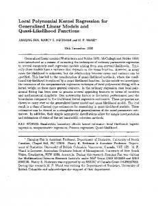
estimate. Our estimate is the local weighted estimate. They are approximately parallel when the smoking package year (X) is smaller than 40, but not so elsewhere. Because in this example the selection probabilities depend mainly on the disease status, parallelism of weighted and unweighted estimates is expected. The reason that our estimate has a different flatness from that of Prentice and Pyke for X ≥ 40 is due to the nonparametric estimation, which is not restricted by the linear logit model. 5. Simulation studies. We conducted simulations to better understand the finite-sample performance of the weighted estimator and the finite-sample effect due to estimating the selection probabilities. Recall that µ CC is the unweighted method which applies the local linear smoother of Fan, Heckman and Wand (1995) directly to the validation set only. We compare the biases and variances of µ CC , µ · π and µ · π . We first consider the case of continuous response Y. We generated n = 200 X’s from a uniform −1 1 distribution, and the response variable Y’s follow the linear link such that Yi = µXi + 3εi , where µxi = x2i , εi i = 1 n is a random sample from normal 0 1 distribution and is independent of Xi . The selection probability given Y is from the logistic model with intercept 0.0 and slope 1.0. Approximately 42% of the data are missing under the above selection probabilities. We ran 1,000 independent replicates in this simulation experiment, and we applied the linear link and logit link to estimate µ· and π·, respectively. In each replicate, µ CC ·, µ · π and µ · π were obtained using the Epanechnikov kernel function Ku = 751 − u2 on −1 1 and the bandwidth selection criteria as described in Section 3.3. The empirical biases of the estimators are shown in Figure 2 for x ∈ −1 1. The curves are the averages of the bias estimates over 1,000 runs. Note that the CC analysis has considerable bias and that µ · π and µ · π are very close in most points. Figure 3 shows the sample variances of µ x π and µ x π . It appears that the weighted estimator using estimated selection probabilities is at least as efficient as the one using the true π·. There is considerable gain using estimated π for a range of X values, especially when X is around zero. The relative efficiency of µ x π to µ x π at x = 0 is 1.29 when n = 200. If we increase the sample size to n = 2000, then the corresponding relative efficiency is 1.22. In Section 6, we explain the finite-sample efficiency gain from estimating the selection probabilities by a second-order variance approximation. We have also investigated the case when the response is binary, and the findings are similar to those for continuous response. We omit the details here. 6. Second-order variance approximation. The simulations in the previous section show that there is finite-sample gain from estimating the selection probabilities. Recall that the first-order asymptotic result of Theorem 1 shows no asymptotic efficiency gain from estimating the selection probabilities. To explain this, we now present the second-order variance approximation. The proof is given in the Appendix.


Fig. 2.

1037

Simulation study for biases from estimating µ for continuous response.

Theorem 2. Under the same conditions as in Theorem 1 and for any x ∈ suppfX with var µx π < ∞, there exists µ ∗ x = µ x π + op h1/2 n−1/2 , such that var µ∗ x = var µx π − n−1 vx1 + o1 for some vx > 0. Theorem 2 shows that using the estimated selection probabilities improves the efficiency at the rate of n−1 . Note that the second-order efficiency gain is valid even when Y is a lattice random variable. For a fixed point x, let the relative efficiency gain by using the estimated selection probabilities be defined by var µx π − var µ∗ x / var µ∗ x . It is easy to see from Theorem 2 that the relative efficiency gain is of order Oh, which goes to zero slowly. This supports the results of our simulations.

1038


Fig. 3.

Simulation study for variances from estimating µ for continuous response.

7. Generalizations. Theorem 1 is a special case of a general phenomenon, which we outline here. Suppose that one has interest in a function η·. If a nuisance function π· were known, one would estimate η· at x by solving a local estimating equation of the form (7)

0 = n−1

n i=1

˜ i πZi β0 + β1 Xi − x 1 Xi − x t Kh Xi − x5Y

where 5 is an estimating function, Z is the covariate variable for π· and ˜ represents a vector which may or may not include Z. We note that in (7), Y 0 = η x. Equation we are primarily interested in the estimation of β0 and β (7) includes the weighted estimating equation obtained from the derivation of ˜ and Z equal the response Y. (3). In our problem, both Y


1039

Now suppose that πz is also estimated by a local estimating equation but with bandwidth λ, so that 0 = n−1

n i=1

˜ i Xi α0 + α1 Zi − z 1 Zi − z t Kλ Zi − z7Y

z. The estimating for some function 7 such that the resulting estimate α0 = π functions 5 and 7 are assumed to satisfy

˜ πZ ηX 0 = E 5Y

˜ X πZ Z 0 = E 7Y

Under this setup, in Appendix C we sketch a result showing that 1. the bias of η x is of order h2 , is independent of the design densities of Z X, but is generally affected by the estimation of π·. 2. the variance of η x is asymptotically the same as if π· were known. Both these conclusions are reflected in our Theorem 1. The extension to multivariate covariates may be made by applying the multivariate kernel function as in Fan, Heckman and Wand (1995, Section 3.2). However, the curse of dimensionality may occur. A more appealing approach is to consider a regression model by the generalized partial linear single-index model [Carroll, Fan, Gijbels and Wand (1997)]. Asymptotic distribution theory in this setting requires further investigation.

APPENDIX: TECHNICAL PROOFS A. Proof of Theorem 1. First, we present a brief proof of the limit distribution of µ · π. The readers are referred to Fan, Heckman and Wand (1995) for some related calculations. Recall that we use known π now. Define ρx = g µx 2 Vµx −1 , and let qi x y = ∂i /∂xi Qg−1 x y . Fan, Heckman and Wand (1995) noted that qi is linear in y for a fixed x and that q1 ηx µx = 0 and q2 ηx µx = −ρx. Conditions. (A1) The function q2 x y < 0 for x ∈ R and y in the range of the response variable. (A2) The functions fX , η3 , varYX = ·, V2 and g3 are continuous. (A3) For each x ∈ suppfX , ρx, varYX = x and g µx are nonzero. (A4) The kernel function K is a symmetric probability density with support −1 1 . (A5) For each point x0 on the boundary of suppfX , there exists a nontrivial interval ⺓ containing x0 such that inf x∈⺓ fX x > 0. (A6) The selection probability πy > 0 for all y ∈ suppfY . (A7) Eq1 ηX1 Y1 δ1 /π1 2+ε < ∞ for some ε > 0.

1040


Proof of the asymptotic distribution of µ · π. We study the asymp∗ 1/2 totic properties of β = nh β0 − ηx hβ1 − η x t . Let ηx u = ηx + η xu−x, X∗i = 1 Xi −x/h t and β∗ = nh1/2 β0 −ηx hβ1 −η x t . 0 β 1 maximizes (3), Since β0 + β1 Xi − x = ηx Xi + nh−1/2 β∗t X∗i , if β ∗ maximizes then β n

(8)

i=1

Qg−1 ηx Xi + nh−1/2 β∗t X∗i Yi

δi K X − x πi h i

as a function of β∗ , where πi = πYi . We consider the normalized function ln β∗ π =

(9)

n

i=1

Qg−1 ηx Xi + nh−1/2 β∗t X∗i Yi

δ

− Qg−1 ηx Xi Yi

i

πi

Kh Xi − x

∗ = β ∗ π maximizes ln · π Let Then β Wn π = nh−1/2

(10)

An π = nh−1

(11)

n i=1

n i=1

q1 ηx Xi Yi

q2 ηx Xi Yi

δi K X − xX∗i πi h i

δi K X − xX∗i X∗t i πi h i

Similarly to Fan, Heckman and Wand (1995), we have that ln β∗ π = Wtn πβ∗ + 12 β∗t An πβ∗ + Op nh−1/2 = Wtn πβ∗ − 12 β∗t