At row 2n in the cellular automaton rule 30, a region of the initial con- dition reappears on the right side, which causes the automaton to âbegin againâ locally.
Local Nested Structure in Rule 30 Eric S. Rowland
Department of Mathematics, Rutgers, The State University of New Jersey, Piscataway, NJ 08854, USA At row 2n in the cellular automaton rule 30, a region of the initial condition reappears on the right side, which causes the automaton to “begin again” locally. As a result, local nested structure is produced. This phenomenon is ultimately due to the property that rule 30 is reversible in time under the condition that the right half of each row is white. The main result of the paper establishes the presence of local nested structure in k-color rules with this bijectivity property, and we explore a class of integer sequences characterizing the nested structure. We also prove an observation of Wolfram regarding the period length doubling of diagonals on the left side of rule 30.
1. Introduction
A one-dimensional cellular automaton consists of a row of cells that are updated in parallel according to a rule icon such as ��� ��� ��� ��� ��� ��� ��� ��� , � � � � � � � � which specifies the color of a cell in terms of the colors of itself and a number of its neighbors on the previous step. The icon above is that of rule 30 and can be paraphrased as follows. If a cell and its right neighbor are both white, the cell becomes the color of its left neighbor; otherwise it becomes the opposite color of its left neighbor. The rule icon ��� ��� ��� ��� ��� ��� ��� ��� � � � � � � � � is that of rule 90, under which a cell becomes white if its left and right neighbors are the same color and black otherwise. Rules 30 and 90 display qualitatively different nested structures. Let I be the doubly infinite row ��������� consisting of a single black cell at position 1 among a background of white cells. In a sense, this is the simplest nontrivial initial condition, and as such we assume that a cellular automaton is begun from I if no other initial condition is specified. Complex Systems, 16 (2006) 239–258; � 2006 Complex Systems Publications, Inc.
240
E. Rowland
Figure 1. Rule 90 evaluated for 100 steps. Global nested structure is evident: Each part resembles the whole.
Figure 1 shows the beginning of rule 90. The left and right diagonals of rule 90 are periodic with period lengths 2Α . It follows that at row 2n , partial copies of the initial condition I reappear on the left and right sides. Locally, the evaluation continues from these isolated black cells identically as it continues initially from I. The number of cells to which row 2n and I agree increases with n, so a “self-similar” nested structure appears on each side. Since the two copies of the initial condition on row 2n span the entire row, this structure is global: Every part of the automaton resembles some part of the initial condition. Figure 2 shows the beginning of rule 30—a triangular pattern of more or less uniform disorder. As convincingly established by Stephen Wolfram in A New Kind of Science [1], systems like rule 30 defy the intuition that simple programs only produce simple results. Rule 30, despite its simple definition, does not appear to generate a regular pattern. However, there are certain local structures in rule 30 that are predictable. In particular, the right diagonals are periodic with period lengths 2Α . (This is shown in Lemma 2.) Just as in the case of rule 90, this periodicity implies that a small region of the initial condition reappears on the right side of row 2n , and from this the computation continues locally as it does from I. Once again, nested structure arises, but in this case the structure remains local. More precisely, the number of central cells to which row 2n agrees with I grows roughly linearly with n, whereas in the case of rule 90 the growth is exponential. In both cases, the nested structure leads to some level of computational reducibility, but in rule 30 this reducibility is quite restricted. This is to be expected simply on the basis of the perceived computational complexity of the two automata: Rule 90 is performing a relatively simple computation, while rule 30 is presumably performing a computation that cannot be Complex Systems, 16 (2006) 239–258
Local Nested Structure in Rule 30
241
Figure 2. Rule 30 evaluated for 100 steps. No global structure is present, but
there is local nested structure on the right side.
Figure 3. Rule 86: a left–right reflected, left-justified image of rule 30, in which the periodicity of columns can be seen. The leftmost sequence of black cells in each row has been highlighted, showing the local nested structure.
done more quickly. That is, rule 90 is computationally reducible, while rule 30 is almost certainly computationally irreducible. As shown for the general case in section 2, the right nestedness of rules 30 and 90 is a consequence of the left bijectivity of these rules. A Mathematica package for studying left and right bijective rules is available from the author’s web site [2]. The nested structure of rule 30 is more easily seen when each row is shifted right relative to the one below it. After an additional left–right reflection (to put it into the standard form used in later sections), one obtains the range [�2, 0] rule 86 shown in Figure 3. Complex Systems, 16 (2006) 239–258
E. Rowland
242
A nested integer sequence naturally arises from this structure, the following properties of which are proved in section 2. Let ΛI (t) be the length of the maximal leftmost sequence of consecutive black cells in � row t � 1 of rule 86. The sequence �ΛI (t)�t�1 begins 1, 3, 1, 4, 1, 3, 1, 6, 1, 3, 1, 4, 1, 3, 1, 7, 1, 3, 1, 4, 1, 3, 1, 6, 1, 3, 1, 4, 1, 3, 1, 9, 1, 3, 1, 4, 1, 3, 1, 6, 1, 3, 1, 4, 1, 3, 1, 7, 1, 3, 1, 4, 1, 3, 1, 6, 1, 3, 1, 4, 1, 3, 1, 15, . . . and is nonperiodic. It follows by right bijectivity that ΛI (t) � a(ord2 (t)) �
for some (strictly) increasing sequence �a(n)�n�0 , where ordl (t) is the exponent of the largest power of l dividing t. Thus a(n) � ΛI (2n ) for all n, so at least n 1 consecutive black cells follow the infinite white left tail on row 2n � 1 and, consequently, for n 1 at least n consecutive white cells, preceded by a black cell, follow the white left tail on row 2n . That is, at least n 1 central cells of row 2n coincide with I. The values of a(n) for 0 � n � 40 are 1, 3, 4, 6, 7, 9, 15, 16, 24, 25, 27, 29, 34, 36, 37, 39, 41, 43, 48, 49, 51, 54, 55, 58, 60, 63, 64, 66, 69, 70, 72, 74, 77, 79, 80, 82, 84, 86, 90, 91, 93. This sequence characterizes the period lengths of the diagonals on the right side of rule 30 and seems to have additional significance as well, as discussed in section 3. However, it displays no obvious regularity by which the nth term may be computed (even conjecturally) in shorter than exponential time. Indeed, the terms given here were obtained directly by computing the rightmost 121 nonwhite diagonals of rule 30 up to row 240 . In section 2 we formalize our discussion with relevant definitions and prove the main theorem of the paper, which establishes the appearance of nestedness in right and left bijective cellular automata. In section 3 we discuss other initial conditions and corresponding integer sequences. Section 4 gives consideration to other right bijective rules and a possible application to the problem of detecting computational reducibility. The left diagonals of rule 30 are only eventually periodic, and this is not sufficient to produce nested structure on the left side. However, the concept of bijectivity can still be used to obtain some information. In section 5 we prove Wolfram’s observation on the period doubling of left diagonals by studying conditions under which rule 30 is right bijective. 2. Bijectivity and convergence
We adopt Wolfram’s paradigm [1, 3] for studying cellular automata. In particular, we use his numbering convention for cellular automaton rules (in which the rule icon is read in base k) with the following additional Complex Systems, 16 (2006) 239–258
Local Nested Structure in Rule 30
243
notation. The set of k colors will be denoted [k], with the special case [2] � ��, ��. The set [k]� of doubly infinite sequences of cells (indexed by the set of integers �, increasing to the right) is the set of rows. For a row R [k]� , let R(m) be the color of the cell at position m in R, and let R[m1 , m2 ] be the (m2 � m1 1)-tuple (R(m1 ), R(m1 1), . . . , R(m2 )). (We have I(1) � �, and I(m) � � for m 1.) For d1 � d2 , a k-color, range [d1 , d2 ] rule f is one in which a cell may be any of k colors and the color of the cell at position m depends on the colors of the d2 � d1 1 cells at positions m d1 , m d1 1, . . . , m d2 on the previous step. Formally, we allow f to be both a function on (d2 �d1 1)-tuples and a function on rows, with the notation f (xd1 , xd1 1 , . . . , xd2 ) for the function f � [k]d2 �d1 1 � [k] and the notation fR for the function f � [k]� � [k]� , where (fR)(m) � f (R(m d1 ), R(m d1 1), . . . , R(m d2 )). The successor of R under f is fR, and the row S is a predecessor of R under f if fS � R. We generate the image of a cellular automaton with rule f and initial condition R by placing below each row f t R its successor � f t 1 R. By “column m of �f t R�” we mean the sequence �(f t R)(m)�t�0 . A row R is rightful if there exists a cell to the left of which all cells are a single color c; all of the “information” of a rightful row is on the right half. The color c will be called the color of the left tail of R, and often our convention will be that R(m) � c R(1) for m � 0. Analogously, a row is leftful if its left–right reflection is rightful. A row is central if it is both rightful and leftful (allowing the left and right tails to be of different colors). Rightfulness, leftfulness, and centrality are preserved under any finite range rule. For example, the row I � ��������� is rightful with a white left tail. It is also leftful with a white right tail. Therefore it is central (with a central part of length 1). The rule f is right bijective if for every (cd1 , cd1 1 , . . . , cd2 �1 ) [k]d2 �d1 the function x � f (cd1 , cd1 1 , . . . , cd2 �1 , x) on [k] is bijective. Define the left–right reflection of a k-color, range [d1 , d2 ] rule f to be the k-color, range [�d2 , �d1 ] rule g satisfying g(xd2 , . . . , xd1 1 , xd1 ) � f (xd1 , xd1 1 , . . . , xd2 ) for every (d2 � d1 1)-tuple (xd1 , xd1 1 , . . . , xd2 ). We say that f is left bijective if its left–right reflection is right bijective. This positional bijectivity has been considered by Jen [4, 5] and by Wolfram [1] (under the name “one-sided additivity”). Complex Systems, 16 (2006) 239–258
E. Rowland
244
The results in this paper are stated for right bijective rules but hold for left bijective rules mutatis mutandis. Accordingly, we primarily study k-color, range [�d, 0] rules f (with d 0). The color of a cell under such a rule depends on the colors of d 1 cells on the previous step, namely itself and its d nearest left neighbors. (By composing with an appropriate horizontal shift, any k-color, finite range rule can be put into this form.) The advantage of these “shifted” rules is that the columns (rather than the diagonals) are periodic. Right bijectivity allows one to uniquely determine c0 in c � f (c�d , c�d 1 , . . . , c�1 , c0 ), given the colors of all other cells appearing. That is, there is an inverse function f �1 � f (c�d , c�d 1 , . . . , c�1 , x) � x for every d-tuple (c�d , c�d 1 , . . . , c�1 ). Because of this inverse function, the automaton can often be run backward in time (uniquely) as well as forward. We say that a row R has an infinite history under f if for every t 1 there exists S�t such that f t S�t � R. We say that R has an infinite rightful history if every S�t can be chosen to be rightful. Under a right bijective rule, a rightful row has at most one infinite rightful history.
Proposition 1.
Proof. Let f be a right bijective, k-color rule, and let R [k]� be a rightful row with left tail color c and an infinite rightful history under f . It suffices to show the uniqueness of a rightful predecessor S of R having an infinite rightful history under f . By right bijectivity, the left tail color c� of S determines S uniquely. Therefore, to show uniqueness of S it suffices to show the uniqueness of c� . Let G be the directed graph on the vertex set [k] with an edge (i � j) from i to j whenever f (i, i, . . . , i) � j. (In particular, we have the edge (c� � c).) The sequence of left tail colors in the infinite rightful history of R corresponds to a (directed) cycle in G. Since every vertex i [k] has exactly one edge leaving it, there is at most one cycle containing the vertex c. The vertex c� in this cycle preceding c is thus unique. For a right bijective rule f and a rightful row R with an infinite rightful history, let us therefore define f �1 R to be the rightful predecessor of R with an infinite rightful history. (By the proof of Propostion 1, R fails to have an infinite rightful history only when the left tail color of R does not belong to a cycle in G.) One verifies for a range [�d, 0] rule that if R(m) � R(0) for m � 0, then (f �1 R)(m) � (f �1 R)(0) for m � 0. Figure 4 shows rule 30 in the range �50 � t � 50, displayed as a (centered) range [�1, 1] rule. Each row in the infinite leftful history has a white right tail and an eventually periodic left “tail.” Complex Systems, 16 (2006) 239–258
Local Nested Structure in Rule 30
245
Figure 4. The history (upper half) and future (lower half) of rule 30 from a single black cell. While the future is computed down the page by the automaton, the history is computed up the page by the inverse function. As guaranteed by Proposition 1, this history is the unique history with white right tails.
Lemma 1 follows immediately from the bijectivity of f . Lemma 1. Let f be a right bijective, range [�d, 0] rule. Let R and S be rows such that R(m) � S(m) for m < M but R(M) S(M). For every t �, (f t R)(M) (f t S)(M).
That is, under a bijectivity condition, changing the color of a cell in the initial condition causes each subsequent (and precedent) cell in the same column to change color as well. A result of Jen [4, Theorem 4] guarantees the eventual periodicity of columns in any range [�d, 0] cellular automaton with a rightful initial condition. For right bijective rules, the periodicity is not eventual but immediate. Intuitively, this is because periodicity in a column continues uniquely backward in time. We formalize this in the following result, where l(k) � lcm(1, 2, . . . , k). Let f be a right bijective, k-color, range [�d, 0] rule, and let R [k]� . If, in the computation of �f t R�, columns m � d, m � d 1, . . . , m � 1 are periodic with period lengths pm�d , pm�d 1 , . . . , pm�1 respectively, then column m is periodic with period length dividing l(k) � lcm(pm�d , pm�d 1 , . . . , pm�1 ). Lemma 2.
Proof. Let p � lcm1�i�d pm�i , and let cj � (f jp R)(m). If cj � c0 for some j 1, then column m is periodic with period length dividing jp. Thus we would like to show that cj � c0 for some 1 � j � k. To that end, assume that cj c0 for 1 � j < k; we show that ck � c0 . By Lemma 1, cj ci for 0 � i < j < k (because cj � ci would imply cj�i � c0 ). Therefore Complex Systems, 16 (2006) 239–258
E. Rowland
246
�c0 , c1 , . . . , ck�1 � � [k], so we must have ck � ci for some 0 � i < k. Again by Lemma 1, i � 0. �
Let Sn [k]� for each n 0. We say that the sequence �Sn �n�0 converges to a row S [k]� and write Sn � S if for every m there exists N such that for all n N we have Sn (m) � S(m). This is simply bitwise convergence, where every cell eventually stabilizes. Theorem 1 implies that a right bijective cellular automaton with a rightful initial condition exhibits local nested structure on the left side. It identifies a sequence of rows in the automaton that converges to its initial condition, causing the computation to “begin again” locally at each. (One can think of this in terms of p-adic convergence in the exponent.) Again, let l(k) � lcm(1, 2, . . . , k). Let f be a right bijective, k-color, range [�d, 0] rule, and let R [k]� be a rightful row with an infinite rightful history under f . n As n � �, f l(k) R � R.
Theorem 1.
Proof. Without loss of generality, assume that R(m) � R(0) for m � 0. For every m � 0, column m of �f t R� is periodic with period length dividing l(k). It follows from Lemma 2 that for m 0, column m of �f t R� � is periodic with period length dividing l(k)m 1 . Therefore �(f t R)[0, m]�t�0 m 1 m 1 l(k) is also periodic with period length dividing l(k) , so (f R)[0, m] � m 1 R[0, m]. As m � �, f l(k) R � R. If f is right bijective, a nested structure is observed on the left side of �f t R� even without the condition of the theorem that R has an infinite rightful history. However, in this case there exists t0 such that f t0 R has an infinite rightful history, and the theorem applies. In some sense, then, it is more natural to consider an initial condition with an infinite history than one without. An immediate corollary of Theorem 1 is that for every integer r, n f l(k) r R � f r R as n � �. This follows from the uniqueness of rightful successors and (infinite history) rightful predecessors. With a right bijective, k-color rule f specified by context, define ΛR (t) � inf�m � � (f t R)(m 1) R(m 1)�. For rightful R, this is the number of central cells to which f t R agrees with R. Thus ΛR (t) � � ����, where ΛR (t) � � if f t R � R and ΛR (t) � �� if f t R and R have different left tail colors. By right bijectivity, Λf r R (t) � ΛR (t) for all r �. An argument similar to that of Lemma 2 shows � � that the sequence �ΛR (l(k)n )�n�0 is strictly increasing; thus �ΛR (t)�t�0 is nonperiodic, and for n 1 n
(f l(k) R)(n � 1) � R(n � 1). This establishes a lower bound on the computational reducibility proComplex Systems, 16 (2006) 239–258
Local Nested Structure in Rule 30
247
vided by the local nested structure on the left side of a right bijective rule begun from a rightful row. 3. The right side of rule 30
For this section, let f be the 2-color, range [�2, 0] rule 86. The rule icon of f is ��� ��� ��� ��� ��� ��� ��� ��� . � � � � � � � � The beginning of the automaton �f t I� is shown in Figure 3. Rule 30 and f , being equivalent up to left–right reflection and a horizontal shift, are different ways of viewing the same computation. Rule 30 is left bijective, and f is right bijective. We favor f for simplicity of indices. Note that f �1 I � ���������. The sequence of left tail colors under f (being all white) has period length 1. The period length of column 1 is also 1, so the proof of n Theorem 1 implies that (f 2 �1 I)(n 1) � �. That is, there are (at least) n 1 consecutive black cells following the white left tail on row 2n � 1. Let ΙR (t) � min�m 0 � (f t R)(m 1) ��. �
�
We have ΙI (t) � Λf �1 I (t) � ΛI (t 1), so �ΙI (t)�t�0 is the sequence �ΛI (t)�t�1 discussed in section 1. It begins 1, 3, 1, 4, 1, 3, 1, 6, 1, 3, 1, 4, 1, 3, 1, 7, . . . �
and has the structure ΙI (t) � a(ord2 (t 1)) for the sequence �a(n)�n�0 beginning 1, 3, 4, 6, 7, 9, 15, 16, . . . . � The sequences �ΙR (t)�t�0 for other rightful rows R show similar characteristics. For example, the row R � ���������� gives the periodic sequence 2, 1, 2, 1, 2, 1, . . . . The row R � ����������� gives the periodic sequence 1, 2, 1, 2, 1, 2, . . . . For R � �����������, �
�ΙR (t)�t�0 begins 3, 1, 4, 1, 3, 1, 6, 1, 3, 1, 4, 1, 3, 1, 7, . . . , which is � simply �ΙI (t 1)�t�0 since in this case R � fI. To take a more interesting example, let R � ������������. Complex Systems, 16 (2006) 239–258
E. Rowland
248
�
One finds that �ΙR (t)�t�0 begins 1, 6, 1, 3, 1, 4, 1, 3, 1, 7, 1, 3, 1, 4, 1, 3, 1, 6, 1, 3, 1, 4, 1, 3, 1, 8, 1, 3, 1, 4, 1, 3, . . . and then repeats with this period of length 32. In general, the sequence �ΙR (t)� for a rightful row R includes several terms from the sequence �a(n)�, since ΙR (t 1) � 1 whenever ΙR (t) > 1, which causes the sequence to (at least temporarily) mimic �ΙI (t)�. More� over, for every rightful R there is a nondecreasing sequence �bR (n)�n�0 � whose first several terms agree with �a(n)�n�0 and which satisfies the following condition. For every n 0 there exists tn such that for all s � we have ΙR (tn s2n 1 ) � bR (n). That is, �ΙR (t)� is partially nested, but �bR (n)� may be eventually constant (so �ΙR (t)� may be periodic). In the previous examples we have seen two types of behavior: Either � �ΙR (t)�t�0 is periodic or R appears in rule 86 begun from I. Experimental evidence suggests that in fact these are the only two cases. �
If R is a central row with white tails such that �ΙR (t)�t�0 is nonperiodic, then R � f r I for some r 0. Conjecture 1.
The conjecture claims that, when begun from I, rule 86 (and thus rule 30) computes precisely the central rows which yield nonperiodic sequences �ΙR (t)�. The conjecture has been verified for every initial condition R whose central part is at most 24 cells in length. Conjecture 1 is not true for rightful rows in general. We now construct a noncentral row R with the property that ΙR (t) � a(ord2 (3t 1)) for all t �. By construction ΙR (t) < �, so that for every t �, f t R f �1 I. It follows that this row R does not appear in rule 86 begun from I. It suffices to arrange that 2n � 1 � � a(n), even n 0; 3 5 � 2n � 1 ΙR� � � a(n), odd n 1. 3 ΙR�
Let R(m) � � for m � 0 and R[1, 2] � (�, �), so that a(0) � 1 as desired. We construct the remainder of R inductively from left to right, a(n 1) � a(n) cells at a time. Assume therefore that we have defined R[1, a(n) 1] such that the stated condition holds for n. Define R[a(n) 2, a(n 1) 1] so that the condition holds for n 1; right bijectivity provides existence and uniqueness of this (a(n 1) � a(n))-tuple. From position 1, R begins ������������������������������������������. The same procedure can be used to construct a rightful row R with any sequence �ΙR (t)� satisfying the condition on �bR (n)� given previously; Complex Systems, 16 (2006) 239–258
Local Nested Structure in Rule 30
249
that is, this condition is also sufficient for a given sequence to occur as �ΙR (t)� for some rightful R. As we considered �ΙR (t)� for various rows R, we may also consider �ΛR (t)�, and in fact it is ΛR (t), not ΙR (t), that provides the natural generalization of �a(n)�. As suggested by Theorem 1, analogous se� quences �aR (n)�n�0 can be defined by aR (ord2 (t)) � ΛR (t). The sequence �aR (n)� for R � ���������� begins 1, 4, 5, 7, 8, 10, 16, 17, 25, 26, 28, 30, . . . , and for R � ����������� it begins 1, 5, 6, 8, 9, 11, 17, 18, 26, 27, 29, 31, . . . . For the row R � ����������� � fI we find that aR (n) � aI (n). In general, af r R (n) � aR (n) for every r �. The converse of this statement has been verified for initial conditions with central parts at most 10 cells in length; that is, each infinite evaluation of rule 30 seems to have its own unique sequence �aR (n)�. Conjecture 2.
If aR (n) � aS (n) for all n, then R � f r S for some r �.
There seems to be some degree of freedom in the sequences �aR (n)�, but it is unclear by how much their growth rates vary. The central initial conditions ������������������ and ������������������ give some indication, having sequences �aR (n)� that begin 1, 3, 4, 6, 7, 9, 12, 13, 15, 17, 20, 21, 23, 25, 27, 29, . . . and 1, 3, 4, 6, 7, 14, 26, 27, 34, 36, 37, 39, 41, 44, 48, 53, . . . respectively. One can construct sequences of arbitrarily large initial growth. It is not difficult to show that aR (0) � 1 for any nontrivial rightful row R with a white left tail. However, consideration of the initial conditions ������������������ shows that aR (1) takes on all odd values greater than 1, and consideration of the initial conditions ������������������� shows that aR (1) takes on all even values greater than 2. Complex Systems, 16 (2006) 239–258
E. Rowland
250
The slowest growing sequence overall,
� min aR (n)� R rightful
�
, n�0
begins 1, 3, 4, 6, 7, 9, 12, 13, 15, 17, 19, . . . . It would be interesting to have more information on the growth rate of this sequence if asymptotic information cannot be obtained for �aR (n)� in general. 4. Other right bijective rules d 1
d
Of the kk k-color rules depending on d 1 cells, precisely k!k are right bijective, and their rule numbers are given by the following function in Mathematica version 5.1 and later, where s � d 1 (and k � k). RightBijectiveRules[k_, s_] := FromDigits[Join @@ #, k] & /@ Tuples[Permutations[Range[k] - 1], k^(s-1)] The package [2] mentioned in section 1 includes an implementation. In general it suffices to consider rules with a periodic sequence of background colors that includes white (i.e., rules under which a white tail supports an infinite history); all other rules are obtained by permuting the colors. Thus we consider rules begun from the initial condition I. (Another nontrivial simple initial condition is f �1 I, where f is the 2-color, range [�2, 0] rule 86. This initial condition also leads to structure worthy of study, but we do not pursue it here.) The sixteen 2-color, range [�2, 0] right bijective rule numbers are 85, 86, 89, 90, 101, 102, 105, 106, 149, 150, 153, 154, 165, 166, 169, 170. Of these, each of the twelve rules 85, 86, 89, 90, 101, 102, 105, 106, 150, 154, 166, 170 supports an infinite rightful history from I and thus shows local nested structure on the left when begun from a rightful row with a white left tail. Figure 5 shows several columns of these automata in the range �32 � t � 31. The 2-color, range [0, 2] left bijective rules with histories from I are left–right reflections of the range [�2, 0] right bijective rules; their rule numbers are 15, 30, 45, 60, 75, 90, 105, 120, 150, 180, 210, 240. Each of these rules shows local nested structure on the right when begun from a leftful row with a white right tail. Of these, rules 30, 45, and Complex Systems, 16 (2006) 239–258
Local Nested Structure in Rule 30
251
85
86
89
90
101
102
105
106
150
154
166
170
Figure 5. The right bijective, 2-color, range [�2, 0] rules which support an infinite
rightful history from I. Each shows local nested structure on the left side. As in Figure 4, the top half of each image shows the history leading to I, and the bottom half shows the evaluation from I.
75 (the reflections of 86, 101, and 89 respectively) are regarded to be computationally irreducible when begun from I. For rule 101, �aI (n)� begins ��, 1, 2, 4, 5, 7, 9, 13, 14, 20, . . . ; for rule 89, �aI (n)� begins ��, 1, 2, 4, 5, 9, 10, 12, 14, 17, . . . . We now explore the relationship between the computational irreducibility of �f t R� for rightful R and the computational irreducibility of � �aR (n)�n�0 , where f is a k-color rule and aR (ordl(k) (t)) � ΛR (t). Specifically, we examine evidence for the following conjecture. Complex Systems, 16 (2006) 239–258
252
E. Rowland
Let f be a right bijective, k-color rule, and let R [k]� have an infinite rightful history under f . The cellular automaton �f t R� is computationally irreducible if and only if the sequence �aR (n)� is computationally irreducible. Conjecture 3.
Moreover, it appears that �aR (n)� is computationally reducible precisely when it is of exponential growth. The sequence �aR (n)� for a computationally reducible cellular automaton is necessarily computationally reducible. For example, aI (n) � 2n 1 for rule 90. Rules 102, 105, 150, and 154 likewise exhibit global nested structure from I, and the sequences �aI (n)� for these rules are successive powers of 2 as well. This is in contrast to the roughly linear growth of �aI (n)� for the irreducible rules 86, 89, and 101. Conjecture 3 does not only apply to I. Indeed, for rule 90 we have aR (n) � 2n 1 for every nontrivial rightful R with a white left tail. Rule 90 is one of four right bijective, 2-color, range [�2, 0] rules that are additive, that is, satisfies f (x�2 , x�1 , x0 ) f (y�2 , y�1 , y0 ) � f (x�2 y�2 , x�1 y�1 , x0 y0 ), where addition is taken modulo 2 everywhere. The others are rules 102, 150, and 170. The additivity of these rules enables one to compute �f t R� for any R as superpositions of copies of �f t I�. In the case of rule 90, the nested structure of �f t I� (given, for example, by Kummer’s determination of �mt � mod 2) allows the computation of a general cell (f t I)(m) in O(log t) operations; thus one can compute a general cell (f t R)(m) in O(t log t) operations, as opposed to the O(t2 ) operations taken by the automaton. For an additive rule f , it is interesting to note that although the human visual system facilely detects the O(log t) computational reducibility in �f t I�, it often fails to detect the O(t log t) computational reducibility in �f t R� for a general row R. As shown in Figure 6, although the periodicity of columns is evident, these automata do not appear to us as having any global structure. Therefore Conjecture 3 provides a potential criterion for determining reducibility in some cases when our eyes cannot. The right bijective rules 105 and 106 are not additive, so we do not know a priori whether or not each is reducible. Rule 105 yields global nested structure when begun from I, and rule 106 leaves I fixed. Computations for rule 105 show that aR (n) � 2n for n 1, and indeed �f t R� is computationally reducible, since rule 105 is simply rule 150 composed with white–black negation. For rule 106, however, one finds that �aR (n)� tends to grow roughly linearly, and there are no properties of rule 106 that suggest the possibility of a computational reduction. Thus, in agreement with Conjecture 3, for right bijective cellular automata it would appear that by examining �aR (n)� one can distinguish both reducible nested (O(log t)) behavior from irreducible uniformly disordered “class 3” (O(t2 )) behavior (in Wolfram’s classification [1, Complex Systems, 16 (2006) 239–258
Local Nested Structure in Rule 30
90
102
253
150
170
Figure 6. The 2-color, range [�2, 0] rules which support white tails and are both
right bijective and additive. In the nontrivial cases, the human visual system apparently fails to detect the O(t log t) computational reducibility of these rules when begun from rightful initial conditions which are not especially simple. The criterion given in Conjecture 3, however, does detect this reducibility.
Figure 7. The 2-color, range [�3, 0] rule 42586 from I, rotated so that time
increases to the right.
6]) and also reducible uniform (O(t log t)) behavior from irreducible uniform (O(t2 )) behavior. We proceed to consider rules with other values of k and d. The 2-color, range [�1, 0] right bijective rule numbers are 5, 6, 9, and 10. Of these, rules 5, 6, and 10 support infinite histories from I. Begun from I, rules 5 and 10 give periodic patterns, and rule 6 gives a global nested pattern. There are 192 2-color, range [�3, 0] right bijective rules that support a rightful history from I. Of these, 25 have eventually constant sequences �aI (n)�; these correspond to structures like vertical lines. An additional 48 rules have sequences �aI (n)� that approximately double with each successive entry, and all of these sequences and corresponding automata are reducible. Several of the remaining 119 rules are shown in Figure 8. Only one of these 119 appears to be computationally reducible upon visual inspection; this is rule 42586 (shown in Figure 7), for which �aI (n)� begins 2, 3, 5, 8, 10, 18, 20, 38, 40, 78, 80, 158, 160, 318, 320, 638, . . . and for n 1 is given by � � �5 � 2(n�1)/2 � 2, if n is odd; aI (n) � � � �5 � 2(n�2)/2 , if n is even. � That is, �aI (n)� is computationally reducible, but it grows slower than 2n . Rule 42586 from I is quite similar to the 2-color, range [�2, 0] Complex Systems, 16 (2006) 239–258
E. Rowland
254
22886
25945
27238
38554
39258
39526
42646
42650
43418
43670
Figure 8. Some of the more interesting irreducible right bijective, 2-color, range [�3, 0] rules which support an infinite rightful history from I. The row I appears as the center row of each. In some, the nested structure on the left is clear; in others it is more difficult to discern. Complex Systems, 16 (2006) 239–258
Local Nested Structure in Rule 30
255
rule 106 begun from R � ����������, which gives for n 1 � � if n is odd; �3 � 2(n�1)/2 , aR (n) � � � �3 � 2(n�2)/2 1, if n is even. � These rules have initial conditions for which they are reducible, but for most initial conditions they appear not to be. (That �aR (n)� grows slower than 2n in reducible cases may prove to be an indication of this phenomenon.) In section 1 we noted that rule 90 displays global nested structure, while the only nested structure of rule 30 appears on the right. One may wonder whether there are rules that are both right bijective and left bijective (so that they display nested structure on both the left and right sides) but that do not display global structure when begun from a central row. The answer is affirmative, and three are found among 2-color, range [�3, 0] rules; their rule numbers are 22185, 27285, and 43350. Therefore, double-sided local nested structure does not force global nested structure. There are 136 3-color, range [�1, 0] right bijective rules that support a rightful history from I. By visual inspection, 42 of these are computationally irreducible when begun from I, and again these coincide with those predicted to be irreducible by Conjecture 3. As one systematically examines rules in this manner, it becomes apparent that Wolfram’s behavioral class 4 (characterized by persistent “particle-like” structures) does not appear among right bijective automata. The only class 4, 2-color, range [�2, 0] rules with white backgrounds are 110 and its left–right reflection, rule 124. Neither of these rules exhibits positional bijectivity or nestedness. For rule 124 we have ΛI (t) � 1 for all t 0; this is simply because each row after the first begins with two black cells. Similarly, the presumed computationally irreducible 2-color, range [�3, 0] automata and 3-color, range [�1, 0] automata are exclusively of Wolfram’s behavioral class 3 as opposed to class 4. Perhaps this is indicative of a deeper relation between the local computational reducibility provided by Theorem 1 and the classes of computation that can be carried out. It is intuitively plausible that, like global nestedness, local nestedness is too restrictive to allow particle-like structures that would otherwise move without constraint. 5. The left side of rule 30
The right side of rule 30 is characterized by periodicity and preservation of information; this is due to the right bijectivity of the rule. A Complex Systems, 16 (2006) 239–258
E. Rowland
256
Figure 9. Rule 30, left-justified. The columns are eventually periodic, with period doublings occurring as prescribed by Proposition 2.
consequence of Jen’s Theorem 4 [4] is that each left diagonal of rule 30 is eventually periodic with period length a power of 2, and the left side is characterized by eventual periodicity and loss of information. From the leftmost nonwhite diagonal, the sequence of eventual period lengths begins 1, 1, 1, 2, 1, 2, 2, 1, 4, 1, 4, 4, 4, 4, 4, 4, 4, 4, 4, 4, 4, 4, 4, 2, 4, 4, 4, 4, 1, 8, 1, 8, 8, 8, 8, 8, 8, 8, 8, 8, 8, 8, 8, 8, 8, 4, 8, 8, . . . . Wolfram [1, page 871] states the following. “Each period doubling turns out to occur exactly when a diagonal in the pattern eventually becomes a white stripe, and the diagonal to its left has an odd number of black cells in each repeating block.”
Proposition 2.
This section is devoted to proving this observation, which holds for rule 30 begun from any rightful row R. Let f be the 2-color, range [�2, 0] rule number 30; this is the leftjustified version, whose rule icon is ��� ��� ��� ��� ��� ��� ��� ��� . � � � � � � � � One hundred rows of �f t I� are shown in Figure 9. Let R and S be rows that differ only at position m. We say that the bit R(m) has a long term effect on its column if for all t 0 we have (f t R)(m) (f t S)(m). By Lemma 1, a bijectivity condition suffices to ensure a long term effect. Because f is not right bijective, one expects that under most circumstances flipping a bit will not have a long term effect on its column, that is, there will eventually be a loss of information in that column. The following bijectivity condition (deduced from the rule icon) describes when there is a long term effect: The value of f (c�2 , c�1 , x) Complex Systems, 16 (2006) 239–258
Local Nested Structure in Rule 30
257
is independent of x if and only if c�1 � �; that is, f (c�2 , c�1 , �) f (c�2 , c�1 , �) if and only if c�1 � �. This gives the following lemma. The bit (f t0 R)(m) has a long term effect on column m precisely when column m � 1 is white for t t0 . Lemma 3.
Further, we observe from the rule icon that f (c�2 , �, x) x if and only if c�2 � �. That is, under the bijectivity condition, a bit flips from one row to the next precisely when its next-nearest left neighbor is black. Consider columns m�2 and m�1 with respective period lengths 2Αm�2 and 2Αm�1 beginning at t � t0 . Set Α � max(Αm�2 , Αm�1 ). Column m has eventual period length 2Αm , with Αm � Α 1. We show that Αm � Α 1 if and only if (f t R)(m � 1) � � for all t t0 and �� � ���t0 � t < t0 2Α � (f t R)(m � 2) � ����� is odd. It is clear that this condition implies that Αm > Αm�2 � Α: Information will be preserved by the bijectivity condition, and the odd number of black cells in the period of column m � 2 guarantees that (f t0 R)(m) Α (f t0 2 R)(m). We now prove the converse. Assume that Αm � Α 1, so that Α Α (f t0 R)(m) (f t0 2 R)(m). The color of (f t0 s�2 R)(m) for s 1 then depends on the parity of s. In particular, Α
Α
(f t0 s�2 R)(m) (f t0 (s�1)2 R)(m), Α
so information regarding the color of (f t0 (s�1)2 R)(m) must propagate down column m from row t0 (s � 1)2Α to row t0 s � 2Α , implying that a bijectivity condition is met. By Lemma 3, (f t R)(m � 1) � � for t t0 , and it follows that the number of black cells in the period of column m � 2 is odd. This completes the proof of Proposition 2. When column m � 1 is eventually white and the eventual period of column m contains at least one black cell, it follows also that column m 1 is eventually black, since f (�, �, x) � � and f (�, x, �) � � for both colors x. Upon examining the long term behavior for several initial conditions, one is tempted to conjecture that among nontrivial rightful rows R with a white left tail, the eventual period of column m in �f t R� is independent of R — that there is really only one “left side” of rule 30, regardless of which rightful initial condition we choose. However, this conjecture is likely false. Since column 1 is black with period length 1, to prove such a conjecture inductively it would suffice to show that the eventual period of column m is independent of R under the assumption that the same is true for all columns to the left of column m. Only under the condition of Lemma 3 is any information regarding the initial condition of column m Complex Systems, 16 (2006) 239–258
E. Rowland
258
retained; therefore, unless column m � 1 is eventually white, the period of column m depends only on the periods of columns m � 2 and m � 1 and so is independent of R. Thus any counterexample to this conjecture occurs when column m � 1 is eventually white. If the period length of column m is greater than the period length of column m � 2, then the period of column m is invariant under white–black negation and thus is independent of R. If not, then by Proposition 2 the number of black cells in the period of column m � 2 is even. It turns out that this case first occurs at column m � 53209: Column 53208 is eventually white, and the period of column 53207 is (�, �, �, �, �, �, �, �, �, �, �, �, �, �, �, �), resulting in two possible periods that might occur as the eventual period of column 53209 and providing a counterexample to the conjecture (if in fact they do occur for some initial conditions). Moreover, each of these periods leads to two other possible periods (at columns 58288 and 72577 respectively), and one surmises that in fact there are infinitely many possible left sides of rule 30. Acknowledgments
I would like to thank Todd Rowland for helpful revision suggestions. References [1] Stephen Wolfram, A New Kind of Science (Wolfram Media, Inc., Champaign, IL, 2002). [2] Eric Rowland, BijectiveRules [a package for Mathematica] (available from http://math.rutgers.edu/�erowland/programs.html). [3] Stephen Wolfram, “Statistical Mechanics of Cellular Automata,” Reviews of Modern Physics, 55 (1983) 601–644. [4] Erica Jen, “Global Properties of Cellular Automata,” Journal of Statistical Physics, 43 (1986) 219–242. [5] Erica Jen, “Aperiodicity in One-dimensional Cellular Automata,” Physica D, 45 (1990) 3–18. [6] Stephen Wolfram, “Universality and Complexity in Cellular Automata,” Physica D, 10 (1984) 1–35.
Complex Systems, 16 (2006) 239–258