Local Relevance Weighted Maximum Margin Criterion for Text Classification Quanquan Gu∗ Abstract Text classification is a very important task in information retrieval and data mining. In vector space model (VSM), document is represented as a high dimensional vector, and a feature extraction phase is usually needed to reduce the dimensionality of the document. In this paper, we propose a feature extraction method, named Local Relevance Weighted Maximum Margin Criterion (LRWMMC). It aims to learn a subspace in which the documents in the same class are as near as possible while the documents in the different classes are as far as possible in the local region of each document. Furthermore, the relevance is taken into account as a weight to determine the extent to which the documents will be projected. LRWMMC is able to find the low dimensional manifold embedded in the high dimensional ambient space. In addition, We generalize LRWMMC to Reproducing Kernel Hilbert Space (RKHS), which can resolve the nonlinearity of the input space. We also generalize LRWMMC to tensor space which is suitable for a new document representation, named tensor space model (TSM). On the other hand, in order to utilize the large amount of unlabeled documents, we also present a Semi-Supervised LRWMMC, which aims to find a projection inferred from the labeled samples, as well as the unlabeled samples. Finally, we present a fast algorithm based on QR-decomposition to make the methods proposed in this paper apply for large scale data set. Encouraging experimental results on benchmark text classification data sets indicate that the proposed methods outperform many existing feature extraction methods for text classification.
Keywords Local Relevance Weighted Maximum Margin Criterion, Feature Extraction, Text Classification, SemiSupervised Learning, Kernel, Tensor 1 Introduction Text classification [1] is one of the core issues in information retrieval and data mining. In text classification, an initial data set of pre-classified documents is partitioned into a training set and a testing set that are subsequently used to construct and evaluate classifiers. For high dimensional text classification problems, a dimensionality reduction phase is often applied so as to reduce the size of the document representations. This has both the effect of reducing over fitting, and learning ∗ State
Key Laboratory on Intelligent Technology and Systems, Tsinghua National Laboratory for Information Science and Technology (TNList), Department of Automation, Tsinghua University, Beijing, China 100084,
[email protected],
[email protected].
Jie Zhou∗ a semantic latent subspace. Dimensionality reduction techniques include two types: (1) feature selection: to select a subset of most representative features from the input feature set [2] [3], and (2) feature extraction: to transform the input space to a smaller feature space. Compared with feature selection, feature extraction can not only reduce the dimensionality of the input space, but also exploit the latent semantic subspace of the input space. Many feature extraction methods [4] [5] [6] [7] [8] [9] [10] [11] have been proposed in the past decades, however, most of these methods assume that the documents are sampled from a Euclidean space. Recent studies suggest that the documents are actually sampled from a nonlinear low-dimensional manifold which is embedded in the high-dimensional ambient space [12] [13]. In this paper, we proposed a feature extraction method, named Local Relevance Weighted Maximum Margin Criterion (LRWMMC) for text classification. It aims to learn a subspace in which the documents in the same class are as near as possible while the documents in the different classes are as far as possible in the local region of each document. Furthermore, the relevance is taken into account as a weight to determine the extent to which the documents will be projected. LRWMMC not only inherits the good property of Maximum Margin Criterion [11], but also is able to find the low dimensional manifold embedded in the high dimensional ambient space. Due to the nonlinearity of the input space, linear method usually cannot map the documents to a subspace, such that the documents in the same class are near enough while the documents in the different classes are far enough. Kernel method [14] alleviates this problem by first mapping the input space to a high dimensional feature space, and then finding a subspace of the feature space. In [15], a kernel LSI was proposed, called Latent Semantic Kernel (LSK). In this paper, we generalize LRWMMC to Reproducing Kernel Hilbert Space (RKHS) [14], named Kernel LRWMMC, which can resolve the nonlinearity of the input space. All the methods mentioned above are based on the document representation, named Vector Space Model (VSM). Recently, a novel document representation,
1136
Copyright © by SIAM. Unauthorized reproduction of this article is prohibited.
named Tensor Space Model (TSM) [16], was proposed, which can exploit the high order correlation between words and may be a potential direction of text representation. Hence, we also generalize LRWMMC to tensor space, named Tensor LRWMMC. On the other hand, while text classification frees organizations from the need of manually organizing document databases, it still needs professionals to label a large enough training data set for learning a classifier, which requires much expensive human labor and much time. Furthermore, compared with the large amount of documents increasing every day, the labeled samples are always insufficient. To address this problem, semisupervised learning [17], which aims to learn from partially labeled data, provides a solution. In this paper, we present a Semi-Supervised LRWMMC, which aims to learn a subspace, inferred from the labeled samples, as well as the unlabeled samples. Finally, a fast algorithm based on QRdecomposition is presented to make the methods proposed in this paper apply for large scale data set. Encouraging experimental results on benchmark text classification data sets indicate that the proposed methods outperform many existing feature extraction methods for text classification. The remainder of this paper is organized as follows. In Section 2, we will review some methods closely related to our method. In Section 3 we will propose a feature extraction method named Local Maximum Margin Criterion for text classification. We generalize LRWMMC to RKHS and tensor space in Section 4 and Section 5 respectively. In Section 6, we present Semi-Supervised LRWMMC. Finally, we present a QRdecomposition based fast algorithm in Section 7. The experiments on standard text classification datasets are demonstrated in Section 8. Finally, we draw a conclusion in Section 9.
in document di , idfj denotes the number of documents containing word wj , and n denotes the total number of documents in the corpus. In addition, xi is normalized to unit length. Using xi as the ith column, we construct the d × n term-document matrix X. This matrix will be used to conduct text classification. In text classification literature, the most popular feature extraction method is Latent Semantic Indexing (LSI) [4]. It aims to learn a subspace by minimizing the mean squared error in which sense it is equivalent to Principal Component Analysis (PCA). However, LSI does not take into account the class information, it is an unsupervised method and it does not always perform well, sometimes even worse than original term vector [18]. To address this problem, several variants of LSI integrating the class information were proposed. [5] first proposed the concept of local LSI, which performed SVD on a local region of each class so that the most important local structure, which is crucial in separating relevant documents from irrelevant documents, could be captured. A drawback is that the local region is defined by only relevant/positive documents which contain no discriminative information, which makes the improvement of classification performance very limited. [6] extended the local region by introducing some irrelevant/negative documents which are the most difficult to be distinguished from the relevant documents and is found to be more effective than using only relevant documents. [7] proposed a Local Relevance Weighted LSI (LRW-LSI) method which gives different weight to each document in the local region according to its relevance. It should be noted that these local LSI methods mentioned above have to perform a separate SVD in the local region of each class, thus they use different projections for different testing documents. [8] proposed a clustered LSI (CLSI) based on low rank matrix approximation. Based on CLSI, [9] proposed a Centroid Representatives (CM) method for text classification. 2 Related Works Linear Discriminant Analysis (LDA) is a famous feature extraction method. It aims to learn a subspace, In this section, we will briefly review the methods in which the between class variance is maximum while mostly related with ours. the within class variance is minimum, i.e. The Vector Space Model (VSM) is widely used for document representation. In VSM, each docu(2.2) max tr((AT Sw A)−1 (AT Sb A)), ment is represented as a bag of words. Let W = {w1 , w2 , . . . , wd } be the complete vocabulary set of the where Sb = Pc nl (ml − m)(ml − m)T is called l=1 document corpus after the stop words removal and between-class scatter matrix, ml and nl are mean vector words stemming operations. The term vector xi of doc- and size of class l respectively, m = Pc nl ml is l=1 Pc ument di is defined as the overall mean vector, Sw = l=1 Sl is the withinclass scatter matrix, Sl is the covariance matrix of xi = [x1i , x2i , . . . , xdi ]T class l. The solution of LDA are composed of the n (2.1) ), xji = tji log( eigenvectors of the matrix S−1 w Sb corresponding to the idfj largest eigenvalues. There is little work [18] using LDA where tji denotes the term frequency of word wj ∈ W for document classification. The reason is that LDA
1137
Copyright © by SIAM. Unauthorized reproduction of this article is prohibited.
involves the inverse and eigen-decomposition of large and dense matrices. Most recently, [10] proposed a spectral regression method to train LDA in linear time, which makes applying LDA for document classification practical. However, LDA still suffers several other drawbacks: (1) Small Sample Size (SSS) problem: when the size of the data set is smaller than the dimension of the feature space, the within-class scatter matrix Sw will be singular which makes the generalized eigen-problem unsolvable; (2) it is only optimal in the case that the data distribution of each class satisfies Gaussian assumption with an identical covariance matrix; (3) it can only extract at most c − 1 features where c is the number of classes. The most related method to our work is Maximum Margin Criterion (MMC) [11]. MMC has been shown to be more effective than LDA. It aims to learn a subspace, in which the sample is close to those in the same class but far from those in the different classes, i.e.
3.2 Local Relevant Region Definition MMC assumes that the data points are sampled from a Euclidean space, and treats the data points as a whole. When the data points are sampled from a nonlinear lowdimensional manifold embedded in the high-dimensional ambient space, which is usually the case in document classification [12] [13], MMC may fail to find the correct latent subspace. A natural treatment for the data sampled from a manifold is to deal with the data region by region, based on the assumption that the manifold is locally homeomorphism to a Euclidean space. Rather than considering the local region of each class [5] [6] [7], we consider the local region of each document. Similar settings can be found in [19] [20]. In detail, for each document, we define two kinds of local relevant region.
Definition 3.1. Within Class Local Relevant Region: For each document xi , its within class local (2.3) max tr(A (Sb − Sw )A), relevant region is the set of its k most relevant docwhere tr(·) denotes the matrix trace and AT A = I. We uments which are in the same class. Denoted by can see that there is no need for computing any matrix Nw (xi ) = {xj |yj = yi , 1 ≤ j ≤ k} inversion when optimizing the above criterion. T
3
Local Relevance Weighted Maximum Margin Criterion 3.1 Quantitative Measure of Relevance Although we have mentioned ”relevant” many times, we have not given a quantitative measure of relevance. In this subsection, we give several candidate measures of relevance. The simplest measure of relevance between documents can be calculated by the cosine distance as (3.4)
r(xi , xj ) =
xTi xj . ||xi || · ||xj ||
We can see that the range of relevance is [0, 1]. r(xi , xj ) = 1 if and only if xi = xj , that means xi and xj refer to the same document. And r(xi , xj ) = 0 if and only if xi ⊥ xj , that means there is no common word shared by these two documents. Since xi is normalized to unit length, the cosine distance degenerates to inner product (3.5)
r(xi , xj ) = xTi xj .
The other relevance measures include Information Gain (IG), χ2 statistic (CHI), Mutual Information (MI) and so on. For details of these relevance measures, please refer to [2][3]. In our study, we use Eq.(3.5) as the relevance measure.
Definition 3.2. Between Class Local Relevant Region: For each document xi , its between class local relevant region is the set of its k most relevant documents which are in the different classes. Denoted by Nb (xi ) = {xj |yj 6= yi , 1 ≤ j ≤ k}. 3.3 LRWMMC We aim to learn a subspace in which the documents in the same class are as near as possible while the documents in the different classes are as far as possible in the local region of each document. With the definition of local relevant region, the idea mentioned above can be formulated in a more concise way. That is, we aim to find a subspace in which the documents in the Within Class Local Relevant Region are as near as possible, while the documents in the Between Class Local Relevant Region are as far as possible. Furthermore, the relevance is taken into account as a weight to determine the extent to which the documents will be projected. More concretely, in the Within Class Local Relevant Region, the less relevant two documents are, the more attention we pay for them, pooling them as near as possible in the subspace, while in Between Class Local Relevant Region, the more relevant two documents are, the more attention we pay for them, pooling them as far as possible in the subspace. This idea is formulated by Maximum Margin
1138
Copyright © by SIAM. Unauthorized reproduction of this article is prohibited.
Criterion for each document as follows, X X r(xi , xj )||AT xi − AT xj ||2 −
i
xj ∈Nb (xi )
X
X
i
xj ∈Nw (xi )
(1 − r(xi , xj ))||AT xi − AT xj ||2 .
(3.6)
Using the Lagrangian method, we can easily find that the optimal A in Eq.(3.10) is composed of the m eigenvectors corresponding to the largest m eigenvalues of XLXT . We summarize the LRWMMC method in Algorithm 1. Algorithm 1 Local Relevance Weighted Maximum Margin Criterion Input: Training set {xi , yi }ni=1 , Local Relevant Region size k, desired dimensionality m; Output: A ∈ Rd×m ; 1. Construct the with-class local relevant region and between class local relevant region for each xi ; 2. Calculate the adjacent matrix W by Eq.(3.7), and L = D − W; 3. Calculate the projection A as the m eigenvectors corresponding to the largest m eigenvalues of XLXT .
As we have mentioned above, the range of r(xi , xj ) is [0, 1]. As a result, the weight 1 − r(xi , xj ) in Within Class Local Relevant Region and the weight r(xi , xj ) in Between Class Local Relevant Region are both nonnegative. This makes the Maximum Margin Criterion correct and reasonable. Since in our setting, the Maximum Margin Criterion weighted by relevance is conducted on each document, we call Eq.(3.6) Local Relevance Weighted Maximum Margin Criterion (LRWMMC). The rationale of LRWMMC is shown in Figure 1. By defining an adjacency matrix W (3.7) 3.4 Discussion The advantages of LRWMMC inif xj ∈ Nb (xi ) or xi ∈ Nb (xj ) r(xi , xj ), clude four-fold: r(xi , xj ) − 1, if xj ∈ Nw (xi ) or xi ∈ Nw (xj ) Wij = 0, otherwise. 1. It inherits the properties of MMC, hence it does not suffer from SSS problem, and it can extract more Eq.(3.6) can be formulated as than c − 1 features, etc. X T T 2 ||A xi − A xj || Wij 2. It exploits the local class information, which is more i,j discriminative than global class information; X X = 2 (xTi AAT xi )Wij − 2 (xTi AAT xj )Wij 3. Since LRWMMC considers the local region of each i,j i,j X X document and deals with the data region by region, = 2 tr(AT xi Wij xTi A) − 2 tr(AT xi Wij xTj A) it is able to find nonlinear low-dimensional manifold i,j i,j which is embedded in the high-dimensional ambient X X space; = 2 tr(AT xi Dii xTi A) − 2 tr(AT xi Wij xTj A) i
i,j
4. It takes into account the relevance weight in the = 2tr(A X(D − W)X A) local relevant region, hence it is more reasonable = 2tr(AT XLXT A) and robust, which will be illustrated in detail in the following; (3.8) P where Dii = j Wij is called degree matrix, and L = It is worthwhile noting that, [21] proposed a DisD − W is called graph Laplacian [19]. criminant Neighborhood Embedding (DNE), which is Now we rewrite the Local Relevance Weighted Max- in fact also a variant of MMC. Although in their setimum Margin Criterion (LRWMMC) as ting, the authors constructed two graphs, the essence of DNE is also a local MMC with the adjacency matrix max tr(AT XLXT A) being defined as (3.9) s.t. AT A = I (3.11) if xj ∈ Nb (xi ) or xi ∈ Nb (xj ) 1, If we expand A as A = (a1 , . . . , am ), then Eq.(3.9) is −1, if xj ∈ Nw (xi ) or xi ∈ Nw (xj ) W = ij equivalent to 0, otherwise. m X max aTi XLXT ai Our method is different from theirs. We can see that i=1 our method pays different attentions to the data points in the local relevant region by relevance weight, while (3.10) s.t. aTi ai = 1, aTi aj = 0(i 6= j). T
T
1139
Copyright © by SIAM. Unauthorized reproduction of this article is prohibited.
Figure 1: The rationale of LRWMMC: (a) The original local relevant region of document t (the red circle in the center) (b) Within class relevant region of document t with k = 3; (c) Between class relevant region of document t with k = 3; (d) The resulted subspace after LRWMMC projection. DNE generally pays equal attention to them in both Within Class Local Relevant Region and Between Class Local Relevant Region. DNE fails to exploit the concise relevance information in the local region, which may benefit the classification performance a lot. Furthermore, when the data distribution is sparse in the input space, which is usually the case in text classification, paying equal attention to the data points in the local region may even ruin the feature extraction algorithm. For example, in the Between Class Local Relevant Region, the least relevant data point may be much more irrelevant than the most relevant data point. If we pay as much attention to the least relevant data point as to the most relevant data point, it may prevent us from pooling the data points in the Within Class Local Relevant Region near enough. In our experiment, we will see that the performance of DNE is encouraging only when the size of local relevant region is very small, e.g. k = 1, 3. In contrast, our method performs very well when k varied in a very wide range, e.g. k ∈ [1, 30].
as (4.12)
where K(, ) is a positive semi-definite kernel function. The mostly used kernel functions include: 1. Polynomial Kernel:K(x, y) = (1 + hx, yi)d ; 2
). 2. Gaussian Kernel:K(x, y) = exp(− ||x−y|| σ2 Let Φ = [φ(x1 ), φ(x2 ), . . . , φ(xn )] denote the data matrix in RKHS, then Eq.(3.10) can be written as follows: (4.13)
max
m X
aTi ΦLΦT ai .
i=1
According to Representor Theorem [14], ai are linear combinations of φ(x1 ), . . . , φ(xn ). There exist coefficients αij , j = 1, 2, . . . , n, such that (4.14)
4 Kernel LRWMMC Kernel methods have been widely used in non-linear dimensionality reduction, and also been successfully used for text classification [15]. To this end, we will address kernelization of LRWMMC. Due to the nonlinearity of the input space, linear method usually cannot map the documents to a subspace, such that the documents in the same class are near enough while the documents in the different classes are far enough. Kernel method [14] alleviates this problem by first mapping the input space to a high dimensional feature space, and then finding a subspace of the feature space. In the following, we utilize the kernel trick [14] to generalize LRWMMC to Reproducing Kernel Hilbert Space (RKHS), namely Kernel LRWMMC. We consider the problem in a feature space F induced by some nonlinear mapping φ : Rd → F. For a proper chosen φ, the inner product h, i in F is defined
hφ(x), φ(y)i = K(x, y),
ai =
n X
αij φ(xj ) = Φαi ,
j=1
where αi = (αi1 , αi2 , . . . , αin )T . Submit Eq.(4.14) into Eq.(4.13), we obtain max
m X
aTi ΦLΦT ai
i=1
= max
m X
αTi ΦT ΦLΦT Φαi
i=1
(4.15)
= max
m X
αTi KLKαi ,
i=1
where K is the kernel matrix with element Kij = K(xi , xj ). The optimal αi , 1 ≤ i ≤ m in Eq.(4.15) is the m eigenvectors corresponding to the m largest eigenvalues of KLK. We summarize the Kernel LRWMMC method in Algorithm 2.
1140
Copyright © by SIAM. Unauthorized reproduction of this article is prohibited.
Algorithm 2 Kernel Local Relevance Weighted Maximum Margin Criterion Input: Training set {xi , yi }ni=1 , Local Relevant Region size k, desired dimensionality m, Kernel type, Kernel Parameters; Output: A ∈ Rd×m ; 1. Construct the kernel matrix K on the training set; 2. Construct the with-class local relevant region and between class local relevant region for each φ(xi ); 3. Calculate the adjacent matrix W by Eq.(3.7), and L = D − W; 4. Calculate the projection αi , 1 ≤ i ≤ m as the m eigenvectors corresponding to the largest m eigenvalues of KLK.
RIn ×(I1 ...In−1 In+1 ...IN ) that results by mode-n flattening the tensor A. For example, matrix column vectors are referred to as mode-1 vectors and matrix row vectors are referred to as mode-2 vectors.
5 Tensor LRWMMC All the methods mentioned above are based on Vector Space Model (VSM). Recently, a novel document representation, named Tensor Space Model (TSM) [16], was proposed, which can exploit the high order correlation between words and may be a potential direction of text representation. Hence, we will discuss tensorization of LRWMMC. Several tensor-based methods [22][23][24] have been proposed in machine learning and data mining literature. Here, we generalize LRWMMC to tensor space. Figure 2: Flattening a 3th order tensor, which is Since the proposed approach is mostly based on ten- flattened in 3 ways to obtain matrices comprising its sor algebra (or multi-linear algebra), we first introduce mode-1, mode-2 and mode-3 vectors. the notation and basic definition of tensor algebra. For more details about tensor algebra, please refer to [25]. 5.1.3 Mode-n Product A generalization of the 5.1 Tensor Algebra Scalars are denoted by lower product of two matrices is the product of a tensor case letters (a, b, . . .), vectors by bold lower case let- and a matrix. The mode-n product of a tensor A ∈ ters (a, b, . . .), matrices by bold upper case letters RI1 ×...In ...IN by a matrix U ∈ RIn ×Jn , denoted by (A, B, . . .), and high-order tensors by calligraphic up- A ×n U, is a tensor B ∈ RI1 ×...×In−1 ×Jn ×In+1 ×...×IN per case letters (A, B, . . .). whose entries are (5.16) X 5.1.1 Notation and Terminology A tensor is a (A ×n U)i ...i j i ...i = Ai1 ...in−1 in+1 ...iN Uin jn . 1 n−1 n n+1 N higher order generalization of a vector (first order in tensor) and a matrix (second order tensor). From In general, a tensor X ∈ RI1 ×I2 ...IN can multiply a a multi-linear algebra view, tensor is a multi-linear N I ×J mapping over a set of vector spaces. The order of tensor sequence of matrices {Ui }i=1 ∈ R i i as XQ×1 U1 ×2 N I1 ×...In ...IN A∈R is N , where In is the dimensionality U2 . . . ×N UN , which can be written as X i=1 ×i Ui of the nth order. Elements of A are denoted as for clarity. From the definition above, we can easily find Ai1 ...in ...iN , 1 ≤ in ≤ In . that the mode-n product B = A ×n U can be computed via the matrix multiplication B(n) = UT A(n) , followed 5.1.2 Mode-n Flattening The mode-n vectors of by a re-tensorization to undo the mode-n flattening. a N th order tensor A are the In dimensional vectors obtained from A by varying index in while keeping 5.1.4 Scalar Product The scalar product of two the other indices fixed. The mode-n vectors are the tensors A, B ∈ RI1 ...In ...IN , is defined as hA, Bi = P P column vectors of mode-n flattening matrix A(n) ∈ i1 . . . iN Ai1 ...iN Bi1 ...iN . The Frobenius norm of a
1141
Copyright © by SIAM. Unauthorized reproduction of this article is prohibited.
tensor A is ||A|| =
p
hA, Ai.
5.2 Tensor LRWMMC Given n tensors {X1 , . . . , Xn } ∈ RI1 ×...In ...IN , Tensor LRWMMC aims to find a sequence of projections Uk ∈ RIk ×Jk , which maximizes the LRWMMC in the tensor metric induced by Frobenius norm of a tensor: X
(5.17)
||Xi
i,j
N Y
×k Uk − Xj
k=1
N Y
×k Uk ||2 Wij .
k=1
Such type of optimization can be solved approximately by employing an iterative scheme [22]. In the following, we will adopt such an iterative scheme to solve the optimization problem. \k Given U1 , . . . , Uk−1 , Uk+1 , . . . , UN , denote Yi as
Algorithm 3 Tensor Local Relevance Weighted Maximum Margin Criterion Input: Training set {Xi , yi }ni=1 , Local Relevant Region size k, desired dimensionality J1 , J2 . . . , JN ; Output: A sequence of projections Uk ∈ RIk ×Jk ; 1. Construct the within class local relevant region and between class local relevant region for each Xi ; 2. Calculate the adjacent matrix W by Eq.(3.7); 3. Initialize Uk = Ik where Ik is any Ik × Jk orthogonal matrix; for t = 1 to Tmax do for k = 1 to N do \k (a)Calculate Yi by Eq.(5.18); \k \k (b)Calculate Yi(k) by mode-k flattening of Yi ; P \k (c)Calculate Tk = i,j Wij (Yi(k) −
\k
(5.18) Yi = Xi ×1 U1 . . .×k−1 Uk−1 ×k+1 Uk+1 . . . UN Then Eq.(5.17) can be written as X i,j
=
X
||Xi
N Y
×k Uk − Xj
k=1 \k ||Yi
×k Uk −
N Y
\k
\k
\k
Yj(k) )(Yi(k) − Yj(k) )T ; (d)Calculate the projection Uk as the Jk eigenvectors corresponding to the largest Jk eigenvalues of Tk ; end for end for
×k Uk ||2 Wij
k=1 \k Yj
×k Uk ||2 Wij
i,j
X
a classifier, which requires much expensive human labor and much time. Furthermore, compared with the i,j large amount of documents increasing every day, the X \k \k \k \k = 2tr(UTk Wij (Yi(k) − Yj(k) )(Yi(k) − Yj(k) )T Uk ) labeled samples are always insufficient. That is, in reality, it is possible to acquire a large set of unlabeled i,j T data rather than labeled data. To address this problem, = 2tr(Uk Tk Uk ) semi-supervised learning [17], which aims to learn from (5.19) partially labeled data, provides a solution. Thus, we P extend LRWMMC to incorporate the unlabeled data. \k \k \k \k where Tk = i,j Wij (Yi(k) − Yj(k) )(Yi(k) − Yj(k) )T . In general, semi-supervised learning can be categorized The optimal Uk in Eq.(5.19) is composed of the Jk into two classes: (1) transductive learning: to estimate eigenvectors corresponding to the largest Jk eigenvalues the labels of the given unlabeled data; and (2) inducof Tk . tive learning: to induce a decision function which has a We summarize the Tensor LRWMMC method in low error rate on the whole sample space. Our method Algorithm 3. belongs to inductive learning. Other semi-supervised inductive methods in text classification include Co-EM 6 Semi-Supervised LRWMMC [26] and Semi-Supervised Discriminant Analysis (SDA) Semi-supervised learning, which can exploit the large [27]. Although there are many other semi-supervised amount of unlabeled samples to improve classification, methods such as [28] [29], they are transdutive learning is successfully used in text classification [26]. In this methods, which are not very practical in large scale text section, we will present a semi-supervised version of classification. LRWMMC. Semi-supervised learning is formulated as follows. LRWMMC considers finding the optimal projection Given a point set X = {x1 , . . . , xl , xl+1 , . . . , xn } ⊂ Rd , purely on the labeled training set. While text classifi- and a label set L = {1, . . . , c}, the first l points xi , 1 ≤ cation frees organizations from the need of manually i ≤ l are labeled as yi ∈ L and the remaining points organizing document bases, it still needs professionals xu , l + 1 ≤ u ≤ n are unlabeled. We define another adjacent matrix W(2) for both to label a large enough training data set for learning =
\k
\k
||UTk Yi(k) − UTk Yj(k) ||2 Wij
1142
Copyright © by SIAM. Unauthorized reproduction of this article is prohibited.
Algorithm 4 Semi-Supervised Local Relevance Weighted Maximum Margin Criterion Input: Training set {xi , yi }ni=1 , Local Relevant Region size k, desired dimensionality m; Output: A ∈ Rd×m ; where N (xi ) denotes the k nearest neighbor of xi . W(2) 1. Construct the with-class local relevant region and reflects the pairwise relevance of all the documents. between class local relevant region for each labeled In dimensionality reduction, there is an assumption samples xi ; that nearby points are likely to have the same embed2. Calculate the adjacent matrix W(1) by Eq.(6.23); ding. Thus, a natural regularizer can be defined as 3. Calculate the adjacent matrix W(2) for both labeled and unlabeled samples by Eq.(6.20); X 1 1 (2) (6.21) || q AT xj ||2 Wij . AT xi − q 4. Calculate the projection A as the m eigenvec(2) (2) i,j Djj tors corresponding to the largest m eigenvalues of Dii X(L(1) − λL(2) )XT . (2) where D is the degree matrix corresponding to the adjacency matrix W(2) . This regularization incurs a heavy penalty if relevant documents xi and xj are is d × d, where d is the dimensionality of the data. mapped far apart. Therefore, minimizing it is an And the time complexity of the eigen-decomposition is attempt to ensure that if xi and xj are relevant, then O(d3 ). As a result, when d is very high, e.g. document, AT xi and AT xj are near as well. By similar derivation the eigen-decomposition is very time consuming. To of Eq.(3.8), Eq.(6.21) is equivalent to this end, a fast algorithm is urgently required. To T (2) T alleviate computational complexity, we adopt QR [30] (6.22) 2tr(A XL X A), decomposition, which is also adopted in [31] [32]. In the where L(2) = I − D−1/2 W(2) D−1/2 is the normalized following, we will present a QR-based fast algorithm. It is worthwhile noting that although the following graph Laplacian corresponding to W(2) . Define an adjacency matrix W(1) for labeled sam- derivation is based on Algorithm 1, the QR-based fast algorithm also works for the other methods presented ples in this paper, e.g. Kernel LRWMMC in Section 4 and · ¸ Wl×l 0 Semi-Supervised LRWMMC in Section 6. (1) (6.23) W = , 0 0 Let X = QR be the QR-decomposition of X, where Q ∈ Rd×t has orthonormal columns, i.e. QT Q = I, R ∈ where Wl×l is defined in Eq.(3.7) for l labeled samples. Rt×n is an upper triangular matrix, and t = rank(X) Then the objective function of Semi-Supervised is the rank of X. Then the projection A ∈ Rd×m can Local Maximum Margin Criterion is be expressed as A = QV, where V ∈ Rt×m is arbitrary orthogonal matrix. Substitute A = QV and X = QR max(tr(AT XL(1) XT A) − λtr(AT XL(2) XT A)) into Eq.(3.9), then Eq.(3.9) can be rewritten as (6.24) = max tr(AT X(L(1) − λL(2) )XT A), labeled and unlabeled samples as (6.20) ½ r(xi , xj ), if xj ∈ N (xi ) or xi ∈ N (xj ) (2) Wij = 0, otherwise.
where λ is a positive regularization parameter. The optimal A in Eq.(6.24) is composed of the m eigenvectors corresponding to the largest m eigenvalues of X(L(1) − λL(2) )XT . We summarize the Semi-Supervised LRWMMC method in Algorithm 4. 7 Fast Algorithm The computational complexity of the proposed methods in this paper (except Tensor LWRMMC, since the dimensionality of TSM is usually not very high, e.g. 27 in our experiment, the original algorithm in Algorithm 3 is sufficiently efficient) is high, due to that it involves in the eigen-decomposition of a large matrix, e.g. XLXT in Algorithm 1. More concretely, the size of XLXT
(7.25)
max tr(VT QT QRLRT QT QV) = max tr(VT RLRT V)
where VT V = I. Hence, the optimal V is composed of the the m eigenvectors corresponding to the largest m eigenvalues of RLRT . After we obtain the optimal V, the optimal A can be computed as A = QV. It should be noted that RLRT is of size t × t, which is much smaller than XLXT , since t ¿ d. The time complexity of eigen-decomposition for RLRT is O(t3 ). And the time complexity of OR-decomposition for X is O(t2 n). As a result, the total time complexity of the fast algorithm is O(t3 +t2 n), while the total time complexity of Algorithm 1 is O(d3 ). So the fast algorithm is much more efficient than the original algorithm.
1143
Copyright © by SIAM. Unauthorized reproduction of this article is prohibited.
8 Experiments In this section, we compare our method with the state of the art methods on three benchmark text classification data sets. We choose Nearest Neighbor as the classification algorithm. All of our experiments have been performed on an AMD Athlon 64 X2 dual 4400+ 2.4GHz Windows XP machine with 2GB memory. 8.1 Data Sets We use three publicly available datasets: 1. Reuters215781 We use the ModLewis split of the database into training and testing parts. Since the aim is classification, in which each document belongs to an exclusive category, we discard documents with no label or with multiple labels. Furthermore, those rare classes that do not occur at least once in both training and testing set are discarded. The resulting training set contains 6535 documents, and the test set 2570 documents with 52 document classes. 2. TREC-92 This is the dataset used for the filtering track in TREC-9, the 2000 Text Retrieval Conference. We use a subset of the dataset, namely Ohsumed set. It was pointed out that this set is much more challenging than the Reuters set. By similar preprocessing of Retuters, we get 634 training and 3038 test documents from 63 categories. 3. 20Newsgroup3 We use the 20 Newsgroups sorted by date version. There are 18846 documents, from 20 different newsgroups, with 11314 (60%) training and 7532 (40%) testing.
and recall to measure the classification performance (8.26)
F1 =
2rp . r+p
8.3 Experiment 1 In this experiment, we compare LRWMMC with some state of the art methods, e.g. LSI [4], CLSI [8], CM [9] and DNE [21]. The implementation of LSI, CLSI and CM are based on the toolbox [33]. The implementation of LDA is based on [10]. The implementation of LRWMMC is based on QRdecomposition based fast algorithm. For LRWMMC and DNE, the size of local relevant region k is set by grid search {1, 3, 5, 10, 20, 30, 40, 50}, and the best classification result is selected. The text classification results are shown in Table 2. We can find that LRWMMC outperforms other methods on all the data sets. The outstanding performance of LRWMMC mainly owes to the utilization of discriminate information in the local relevant region of each documents, rather than the discriminate information in the local region of each topic (class). And LRWMMC outperforms DNE due to it takes into account the relevance weight in the local relevant region. Furthermore, we investigate the performance of LRWMMC and DNE with respect to the size of the local relevant region, i.e. k. The results are shown in Figure 3. We can see that the performance of DNE is encouraging only when the size of local relevant region is very small, e.g. k = 1, 3. As k increases, the performance of DNE degenerates very much. In contrast, our method performs very good when k varied in a very wide range, e.g. k ∈ [1, 30]. This advantage mainly owes to the local relevance weight, which makes our method more robust for text classification,
8.2 Evaluation Metrics To evaluate the effectiveness of classification, we firstly calculate the average 8.4 Experiment 2 In this experiment, we compare precision and recall by micro-averaging and macro- Kernel LRWMMC with LSK [15] and Kernel Discriminant Analysis (KDA) [34], which are state of the art averaging [1] in Table 1. kernel methods. The implementation of KDA is based on [34] which is very efficient. The implementation of Table 1: Average precision and recall by micro- Kernel LRWMMC is based on QR-decomposition based averaging and macro-averaging fast algorithm. We use Gaussian kernel for all the kerMicroaveraging Macroaveraging nel based methods. The hyper-parameter σ in Gaussian Pc T Pi Pc i=1 T Pi +F Pi i=1 T Pi kernel is tuned by 5-fold cross validation on the trainP Precesion(p) p = c T Pi +F Pi p = c i=1 Pc T Pi ing set, and the best σ for each method is chosen in the Pc T Pi i=1 T Pi +F Ni Recall(r) r = Pc i=1 r = testing. c i=1 T Pi +F Ni The text classification results are shown in Table 3. We can find that Kernel LRWMMC outperforms And we use the single number metric F1 score [1] LSK and KDA on all the data sets. It should be noted which is defined as the harmonic mean of the precision that Kernel LRWMMC also outperforms LRWMMC, the reason is that by nonlinear mapping, Kernel LR1 http://www.daviddlewis.com/resources/testcollections/ 2 http://trec.nist.gov/data/t9 filtering.html WMMC can find even better projection which projects 3 http://people.csail.mit.edu/jrennie/20Newsgroups/ the documents in the same class as near as possible,
1144
Copyright © by SIAM. Unauthorized reproduction of this article is prohibited.
Method LSI CLSI CM LDA DNE LRWMMC
Table 2: Classification results on Reuters Reuters21578 TREC-9 20Newsgroup Micro-F1 Macro-F1 Micro-F1 Macro-F1 Micro-F1 Macro-F1 0.7319 0.7714 0.4901 0.9018 0.8421 0.4987 0.9371 0.7422 0.8723 0.8222 0.5175 0.5088 0.9156 0.7275 0.8776 0.8315 0.5319 0.5274 0.9267 0.7305 0.8575 0.7828 0.5625 0.5571 0.9421 0.7875 0.9098 0.8504 0.6432 0.6396 0.9552 0.8097 0.9115 0.8886 0.6616 0.6604
1
1
0.8 0.75
0.95
0.95 0.7 0.65
0.9
0.9 microF1
microF1
microF1
0.6 0.85
0.85
0.55 0.5
0.8
0.8 0.45 0.4
0.75
0.75 DNE LRWMMC
0.35
DNE LRWMMC
0.7
0.7 5
10
15
20
25 k
30
35
Reuters21578
40
45
50
DNE LRWMMC
0.3 5
10
15
20
25 k
30
TREC-9
35
40
45
50
5
10
15
20
25 k
30
35
40
45
50
20Newsgroup
Figure 3: Classification results (microF1) with respect to the size of local relevant region, i.e. k.
Method LSK KDA Kernel LRWMMC
Table 3: Classification Reuters21578 Micro-F1 Macro-F1 0.7892 0.9159 0.8067 0.9349 0.9656 0.8129
while the documents in the different classes as far as possible, in the local relevant region of each document. 8.5 Experiment 3 In this experiment, we compare Tensor LRWMMC with High Order SVD (HOSVD) [16]. HOSVD is the generalization of SVD to tensor space. As a result, HOSVD can be seen as generalized LSI for TSM. The construction of the Tensor Space Model (TSM) is according to [16]. More concretely, we use a 3-order tensor to represent each document and index this document by the 26 English letters. All the other characters except the 26 English letters are treated as the same symbol, denoted as ∗. The character string in each document is separated 3 characters by 3 characters with overlap. For example, we separate the following sentence, It said it plans ... as It*,t*s,*sa,sai,aid,id*,d*i,*it,it*,...
results of kernel methods TREC-9 20Newsgroup Micro-F1 Macro-F1 Micro-F1 Macro-F1 0.7875 0.5119 0.8575 0.5174 0.8016 0.5872 0.8821 0.5951 0.9271 0.9043 0.7127 0.7109 Thus, each document is a 27×27×27 3-order tensor, and is normalized to unit length. And the corpus is a 27 × 27 × 27 × n 4-order tensor, where n is the number of documents in the corpus. The text classification results are shown in Table 4. We can find that Tensor LRWMMC outperforms HOSVD on all the data sets. However, when we compare TSM with VSM in Table 2, we find that TSM does not always outperform VSM as we expected. The reason may be that the construction of the TSM is just a preliminary strategy [16]. In the future work, we will investigate other kinds of strategies for constructing the TSM. 8.6 Experiment 4 In this experiment, we compare Semi-Supervised LRWMMC with Co-EM [26] and Semi-Supervised Discriminant Analysis (SDA) [27]. Co-EM is the most popular inductive semisupervised learning algorithm for text classification.
1145
Copyright © by SIAM. Unauthorized reproduction of this article is prohibited.
Table 4: Classification results with tensor representation Reuters21578 TREC-9 20Newsgroup Micro-F1 Macro-F1 Micro-F1 Macro-F1 Micro-F1 Macro-F1 HOSVD 0.8514 0.6917 0.8271 0.7319 0.5172 0.5087 Tensor LRWMMC 0.9133 0.8810 0.6739 0.7649 0.8275 0.6529 Method
The implementation of Semi-Supervised LRWMMC is based on QR-decomposition based fast algorithm. We randomly split the training set into labeled and ”unlabeled” set for semi-supervised learning. And use the testing set for inductive classification. For Reuters21578, we vary the number of labeled samples by {200, 500, 1000, 2000, 3000, 4000, 5000}; for TREC-9, we vary the number of labeled samples by {200, 300, 400, 500, 600}; for 20Newsgroup, we vary the number of labeled samples by {2000, 4000, 6000, 8000, 10000}, and the rest samples are treated as ”unlabeled”. The regularizer λ in Semi-Supervised LRWMMC is set by searching the grid {4−3 , 4−2 , 4−1 , 40 , 41 , 42 , 43 }. The LRWMMC trained on the labeled samples is used as the baseline. Since the labeled samples are randomly chosen, we repeat this experiment 10 times and calculate the average result. The results of inductive classification are shown in Figure 4. We can find that Semi-Supervised LRWMMC outperforms the Co-EM and SDA on all the data sets. It should be noted that as the number of labeled samples increases, the performance of LRWMMC increases dramatically. For Reuters dataset, when the number of labeled samples increases to 4000, and for TREC9 dataset, when that increases to 500, LRWMMC even outperforms Co-EM and SDA. This strengthens the effectiveness of LRWMMC again. 9 Conclusion The contributions of this paper include five folds: (1) We proposed a feature extraction method, named Local Relevance Weighted Maximum Margin Criterion (LRWMMC) for text classification; (2) We presented a Kernel LRWMMC to resolve the nonlinearity of the input space; (3) We presented a Tensor LRWMMC for TSM; (4) We presented a Semi-Supervised LRWMMC, which utilizes both the labeled and unlabeled samples. (5) We presented a fast algorithm for the methods proposed in this paper. Encouraging experimental results on benchmark text classification data sets indicate that the proposed methods are superior to many existing feature extraction methods for text classification.
Acknowledgement This work was supported by the National Natural Science Foundation of China (No.60721003, No.60673106 and No.60573062) and the Specialized Research Fund for the Doctoral Program of Higher Education. We thank the anonymous reviewers for their helpful comments. References
[1] Fabrizio Sebastiani, “Machine learning in automated text categorization,” ACM Comput. Surv., vol. 34, no. 1, pp. 1–47, 2002. [2] Yiming Yang and Jan O. Pedersen, “A comparative study on feature selection in text categorization,” in ICML, 1997, pp. 412–420. [3] Tao Liu, Shengping Liu, Zheng Chen, and Wei-Ying Ma, “An evaluation on feature selection for text clustering,” in ICML, 2003, pp. 488–495. [4] Scott C. Deerwester, Susan T. Dumais, Thomas K. Landauer, George W. Furnas, and Richard A. Harshman, “Indexing by latent semantic analysis,” JASIS, vol. 41, no. 6, pp. 391–407, 1990. [5] David A. Hull, “Improving text retrieval for the routing problem using latent semantic indexing,” in SIGIR, 1994, pp. 282–291. [6] Hinrich Sch¨ utze, David A. Hull, and Jan O. Pedersen, “A comparison of classifiers and document representations for the routing problem,” in SIGIR, 1995, pp. 229–237. [7] Tao Liu, Zheng Chen, Benyu Zhang, Wei-Ying Ma, and Gongyi Wu, “Improving text classification using local latent semantic indexing,” in ICDM, 2004, pp. 162–169. [8] Efstratios Gallopoulos and Dimitrios Zeimpekis, “Clsi: A flexible approximation scheme from clustered termdocument matrices,” in SDM, 2005. [9] Dimitrios Zeimpekis and Efstratios Gallopoulos, “Linear and non-linear dimensional reduction via class representatives for text classification,” in ICDM, 2006, pp. 1172–1177. [10] Deng Cai, Xiaofei He, and Jiawei Han, “Training linear discriminant analysis in linear time,” in ICDE, 2008, pp. 209–217. [11] Haifeng Li, Tao Jiang, and Keshu Zhang, “Efficient and robust feature extraction by maximum margin criterion,” in NIPS, 2003.
1146
Copyright © by SIAM. Unauthorized reproduction of this article is prohibited.
1 0.9
0.8
0.8
0.8
0.7
0.7
0.7
0.6
0.6
0.6
0.5
0.5
0.4
0.4
0.3
0.3
0.2
Co-EM SDA Semi-Supervised LRWMMC LRWMMC
0.1 0
500
1000
1500 2000 2500 3000 3500 number of labeled samples
4000
Reuters21578
4500
5000
microF1
1 0.9
microF1
microF1
1 0.9
0.4 0.3
0.2
0.2
Co-EM SDA Semi-Supervised LRWMMC LRWMMC
0.1 0 200
0.5
250
300
350 400 450 number of labeled samples
TREC-9
500
550
Co-EM SDA Semi-Supervised LRWMMC LRWMMC
0.1
600
0 2000
3000
4000
5000 6000 7000 number of labeled samples
8000
9000
10000
20Newsgroup
Figure 4: Inductive classification results (microF1) with respect to the number of labeled samples. The horizontal axis represents the number of randomly labeled data in the training set. [12] Xiaofei He, Deng Cai, Haifeng Liu, and Wei-Ying Ma, “Locality preserving indexing for document representation,” in SIGIR, 2004, pp. 96–103. [13] Dell Zhang, Xi Chen, and Wee Sun Lee, “Text classification with kernels on the multinomial manifold,” in SIGIR, 2005, pp. 266–273. [14] B. Sch?lkopf and A.J. Smola, Learning with Kernels, MIT Press, Cambridge, MA, USA, 2002. [15] Nello Cristianini, John Shawe-Taylor, and Huma Lodhi, “Latent semantic kernels,” in ICML, 2001, pp. 66–73. [16] Ning Liu, Benyu Zhang, Jun Yan, Zheng Chen, Wenyin Liu, Fengshan Bai, and Leefeng Chien, “Text representation: From vector to tensor,” in ICDM, 2005, pp. 725–728. [17] Xiaojin Zhu, “Semi-supervised learning literature survey,” Tech. Rep., Computer Sciences, University of Wisconsin-Madison, 2005. [18] Kari Torkkola, “Linear discriminant analysis in document classification,” in In IEEE ICDM Workshop on Text Mining, 2001. [19] Shuicheng Yan, Dong Xu, Benyu Zhang, HongJiang Zhang, Qiang Yang, and Stephen Lin, “Graph embedding and extensions: A general framework for dimensionality reduction,” IEEE Trans. Pattern Anal. Mach. Intell., vol. 29, no. 1, pp. 40–51, 2007. [20] Deng Cai, Xiaofei He, Kun Zhou, Jiawei Han, and Hujun Bao, “Locality sensitive discriminant analysis,” in IJCAI, 2007, pp. 708–713. [21] Wei Zhang, Xiangyang Xue, Zichen Sun, Yue-Fei Guo, and Hong Lu, “Optimal dimensionality of metric space for classification,” in ICML, 2007, pp. 1135–1142. [22] Shuicheng Yan, Dong Xu, Qiang Yang, Lei Zhang, Xiaoou Tang, and HongJiang Zhang, “Discriminant analysis with tensor representation,” in CVPR (1), 2005, pp. 526–532. [23] Jimeng Sun, Spiros Papadimitriou, and Philip S. Yu, “Window-based tensor analysis on high-dimensional and multi-aspect streams,” in ICDM, 2006, pp. 1076– 1080.
[24] Jimeng Sun, Dacheng Tao, and Christos Faloutsos, “Beyond streams and graphs: dynamic tensor analysis,” in KDD, 2006, pp. 374–383. [25] Lieven De Lathauwer, Bart De Moor, and Joos Vandewalle, “On the best rank-1 and rank-(r1,r2,. . .,rn) approximation of higher-order tensors,” SIAM Journal on Matrix Analysis and Applications, vol. 21, no. 4, pp. 1324–1342, 2000. [26] Kamal Nigam, Andrew McCallum, Sebastian Thrun, and Tom M. Mitchell, “Text classification from labeled and unlabeled documents using em,” Machine Learning, vol. 39, no. 2/3, pp. 103–134, 2000. [27] Deng Cai, Xiaofei He, and Jiawei Han, “Semisupervised discriminant analysis,” in IEEE 11th International Conference on Computer Vision, 2007, pp. 1–7. [28] Xiaojin Zhu, Zoubin Ghahramani, and John D. Lafferty, “Semi-supervised learning using gaussian fields and harmonic functions,” in ICML, 2003, pp. 912–919. [29] Dengyong Zhou, Olivier Bousquet, Thomas Navin Lal, Jason Weston, and Bernhard Sch¨ olkopf, “Learning with local and global consistency,” in NIPS, 2003. [30] Gene H. Golub and Charles F. Van Loan, Matrix Computation, Johns Hopkins University Press, Baltimore, Maryland, third edition, 1996. [31] Jieping Ye, Qi Li, Hui Xiong, Haesun Park, Ravi Janardan, and Vipin Kumar, “Idr/qr: an incremental dimension reduction algorithm via qr decomposition,” in KDD, 2004, pp. 364–373. [32] Haixian Wang, Wenming Zheng, Zilan Hu, and Sibao Chen, “Local and weighted maximum margin discriminant analysis,” in CVPR, 2007. [33] D. Zeimpekis and E. Gallopoulos, “Tmg: A matlab toolbox for generating term-document matrices from text collections,” Grouping Multidimensional Data: Recent Advances in Clustering, pp. 187–210, 2006. [34] Deng Cai, Xiaofei He, and Jiawei Han, “Efficient kernel discriminant analysis via spectral regression,” in ICDM, 2007, pp. 427–432.
1147
Copyright © by SIAM. Unauthorized reproduction of this article is prohibited.