techniques to find a Nash equilibrium in two-player general- sum games. The algorithm searches for a Nash equilibrium and, if it is stopped before it has found ...
2010 IEEE/WIC/ACM International Conference on Web Intelligence and Intelligent Agent Technology
Local Search Methods for Finding a Nash Equilibrium in Two-Player Games Sofia Ceppi, Nicola Gatti, Giorgio Patrini, Marco Rocco Dipartimento di Elettronica e Informazione Politecnico di Milano Piazza Leonardo da Vinci, 32, 20133, Milano, Italy {ceppi, ngatti}@elet.polimi.it, {giorgio.patrini, marco1.rocco}@mail.polimi.it negligible time (< 1 s). However, there are some classes (e.g., Covariant, Graphical, and Polymatrix) whose instances are hard to be solved with all the algorithms. This is due to three reasons: they search for an equilibrium by enumerating all the possible solutions in a static way, the number of these rises exponentially in the number of agents’ actions, and, in the worst case, the algorithms must explore the whole solution space. In PNS the number of supports rises as 4n and in LH the number of the vertices of the best response polytope rises as 2.6n [9]. The literature deals with computational hardness providing algorithms to compute approximate equilibria [10]. However, it has been shown that also the problem of approximating a Nash equilibrium is PPAD-complete. In the present paper, we propose, to the best of our knowledge, the first anytime algorithm based on the combination of support enumeration methods and local search techniques [11]. We formulate the problem of finding a Nash equilibrium as a combinatorial optimization problem where the search space is the support space and the function to be minimized is designed such that its global minima correspond to Nash equilibria. Basically, our algorithm works by iterative generating new solutions (according to a topological representation of the support space) and accepting those that improve the value of a given objective function. Since the objective function is generally non-convex and presents multiple local optima, metaheuristics are employed to escape from them and to reach a global optimum. We design several dimensions for our algorithm: objective functions (two inspired by operational research concepts returning an infeasibility measure of the associated mathematical programming problem and two inspired by game theory concepts: approximate equilibrium and regret), heuristics (iterative improvement and Metropolis with ad hoc pivoting rules), and metaheuristics (random restart, simulated annealing, tabu search, and variable neighborhood). In our experimental analysis, we isolate hard instances produced with GAMUT that are unsolvable with the above three algorithms within a reasonable time (i.e., two hours) and then we apply our algorithm to such instances evaluating the time needed for finding an equilibrium. We show that our algorithm outperforms LH, PNS, and SGC solving with high probability small-medium games within a short time and
Abstract—The computation of a Nash equilibrium of a game is a challenging problem in artificial intelligence. This is because the computational time of the algorithms provided by the literature is, in the worst case, exponential in the size of the game. In this paper, we present, to the best of our knowledge, the first anytime algorithm based on the combination of support enumeration methods and local search techniques to find a Nash equilibrium in two-player generalsum games. The algorithm searches for a Nash equilibrium and, if it is stopped before it has found an equilibrium, it returns the best approximate equilibrium found so far. We design some dimensions for our algorithm and we experimentally evaluate them. Our algorithm solves with high probability games that are unsolvable with the algorithms known in the literature within a reasonable time and provides good anytime performance. Keywords-Algorithmic game theory, Nash equilibrium, local search techniques
I. I NTRODUCTION Non-cooperative game theory provides models and solution concepts to capture settings in which rational agents strategically interact. The central solution concept is Nash equilibrium [1]. It prescribes strategies such that no agent can gain more by deviating unilaterally from them. Any game is proved to admit at least a Nash equilibrium, however its computation is a challenging problem even with two agents. In [2] the authors show that computing a Nash equilibrium in an n-player game is PPAD-complete. It is generally believed that P≠PPAD and then, in the worst case, computing a Nash equilibrium will take time exponential in the size of the game [3]. In this paper we focus on two-player general-sum strategic-form games with complete information. The literature provides three solving algorithms: LH [4] based on linear complementarity mathematical programming, PNS [5] based on support enumeration, and SGC [6] based on mixed integer linear programming. Each of the above three algorithms outperforms the others in some specific settings: PNS outperforms SGC and LH for almost all the games generated by GAMUT [7]; LH outperforms PNS and SGC for games with medium-large support equilibria; SGC outperforms PNS and LH when one searches for an optimal equilibrium. As shown in [6], [8], the instances of the most game classes (with 150 actions per agent) are solved in a 978-0-7695-4191-4/10 $26.00 © 2010 IEEE DOI 10.1109/WI-IAT.2010.57
335
with small probability large games within a reasonable time. Furthermore, we implement anytime versions of LH, PNS and SGC and we compare them with respect to our algorithm in terms of quality of the best solution found within a given deadline. We show that the anytime performances of our algorithm are better than those of the best anytime version among LH, PNS, and SGC.
∑ p−i (a) ⋅ ui (aj , a) = vi,j
a∈A−i
vi,j = vi vi,j ≤ vi
II. S TATE OF THE A RT A. Games, Solution Concepts, and PNS Algorithm A strategic-form game is a tuple (N, A, u), where: N = {1, . . . , m} is the set of agents; A = (A1 , . . . , Am ) where Ai is the set of actions available to agent i; u = (u1 , . . . , um ) where ui is the utility function of agent i. In this work we focus on two-player games.
b1 64, 63 47, 25 54, 30 79, 10 57, 50
b2 91, 0 46, 62 78, 41 31, 56 26, 62
Figure 1.
b3 25, 63 42, 50 49, 2 77, 31 12, 100
b4 94, 37 38, 80 65, 6 64, 47 44, 58
∀i ∈ {1, 2}, aj ∈ Si ∀i ∈ {1, 2}, aj ∈ Ai /Si
(1) (2) (3)
pi (aj ) ≥ 0
∀i ∈ {1, 2}, aj ∈ Si
(4)
pi (aj ) = 0
∀i ∈ {1, 2}, aj ∈ Ai /Si
(5)
∑ pi (a) = 1
∀i ∈ {1, 2}
(6)
a∈Ai
The hardness of computing a Nash equilibrium pushes for the need for approximate solutions. Fix � > 0, a strategy profile σ = (σ1 , σ2 ) is an �-Nash equilibrium if, for all the agents i and for all the actions a ∈ Ai , we have ui (σi , σ−i ) ≥ ui (a, σ−i ) − �. The meaning is that, if agent i deviates from σi making any available action a with probability of one, then she cannot gain more than �. In our work we use a stronger concept of �-Nash equilibrium, called well-supported �-Nash and defined in [10]. Fix � > 0, a strategy profile σ = (σ1 , σ2 ) is a well-supported �-Nash equilibrium if, for all the agents i and for all the actions a′ ∈ Si and a ∈ Ai , we have ui (a′ , σ−i ) ≥ ui (a, σ−i ) − �. A strategy profile that is a well-supported �-Nash equilibrium is also an �′ -Nash equilibrium with �′ ≤ �, for some �′ > 0. Consider Example 2.1, strategy profile σ = (σ1 , σ2 ) where ⎧ ⎧ ⎪ ⎪ a1 0.1968 a1 0.3133 ⎪ ⎪ ⎪ ⎪ ⎪ ⎪ ⎪ ⎪ ⎪ ⎪ a2 0.1220 a2 0.3608 ⎪ ⎪ ⎪ ⎪ ⎪ ⎪ ⎪ ⎪ σ1 = ⎨a3 0.6812 , σ2 = ⎨a3 0.3259 , ⎪ ⎪ ⎪ ⎪ ⎪ ⎪ ⎪ ⎪ a4 0.0 a4 0.0 ⎪ ⎪ ⎪ ⎪ ⎪ ⎪ ⎪ ⎪ ⎪ ⎪ ⎪ ⎪ a 0.0 ⎩a5 0.0 ⎩ 5
Example 2.1: We consider a two-player strategic-form game where agent 1’s available actions are A1 = {a1 , a2 , a3 , a4 , a5 } and agent 2’s available actions are A2 = {b1 , b2 , b3 , b4 , b5 }. The pairs (x, y)s reported in the bimatrix depicted in Fig. 1 are the payoffs of agent 1 and agent 2, respectively. a1 a2 a3 a4 a5
∀i ∈ {1, 2}, aj ∈ Ai
b5 36, 51 23, 89 71, 22 64, 51 75, 34
Payoff bimatrix of Example 1.
We denote by σi the strategy of agent i. A strategy profile σ = (σ1 , σ2 ) is a Nash equilibrium if, for all the agents i and for all the strategies σi′ , we have ui (σi , σ−i ) ≥ ui (σi′ , σ−i ), where −i denotes the opponent of i. Given a strategy σi , the support Si of agent i is the set of actions played with non-null probability by i and a joint support, denoted by S, is a tuple specifying one support for each agent, namely, S = (S1 , S2 ). In what follows, at first we review the technicalities behind PNS that we use in our work and then the concepts of approximate equilibrium. PNS is a blind search algorithm: it statically scans supports in increasing order of balance and size. (The balance is defined as ∣∣S1 ∣ − ∣S2 ∣∣, while the size of S is defined as ∣S1 ∣+∣S2 ∣.) In order to reduce the search space, conditionally dominated actions are removed, i.e., actions a ∈ Ai for which there is an a′ ∈ Ai such that Ui (a, b) ≤ Ui (a′ , b) for all b ∈ S−i . For each S in which there is no conditionally dominated action, PNS checks whether or not an equilibrium there exists. In two-player complete-information games this problem can be formulated as a linear feasibility problem, where the variables are the probabilities pi (a) with which agent i takes action a, as follows (vi,j denotes the utility expected by agent i from playing action j):
is a well-supported �-Nash equilibrium with � = 16.02 and an �′ -Nash equilibrium with �′ = 5.36. The computation of approximate equilibria in generalsum games is currently an open problem and the literature providing a series of examples more than a coherent set of results, e.g., see [12]. B. Local Search Techniques Local search techniques [11] are tools commonly employed to address combinatorial optimization problems [13]. Essentially, they are heuristic algorithms and produce solutions that are not necessarily optimal, but that can be found within an acceptable amount of time. However, it is worth noting that with several problems (e.g., SAT) local search techniques allow one to handle instances, finding the exact solution, that the fastest non-heuristic search algorithm
336
randomly-generated 3CNF formulas, whereas the fastest systematic search algorithms cannot handle instances from the same distribution with more than 400 variables [15]. We briefly review how a SAT problem can be formulated as a combinatorial optimization problem, being very close to the formulation we propose in this work for the problem of finding a Nash equilibrium. A solution s is a binary vector, e.g., s = [0, 1, . . . , 0], where the i-th position of s is the truth assignment of the i-th variable. Function f is defined as the number of satisfied clauses. Usually, iterative improvement with randomized pivoting is employed to solve SAT. We recall that local search techniques have been applied to the problem of searching for a Nash equilibrium only in very special cases. Exactly, they have been applied to potential games where the minimization of a function (called potential function) with discrete arguments corresponds to a pure strategy Nash equilibrium [16], [17] (these games always admit pure strategy equilibria) and they have been applied to find approximated equilibria in pure-strategies infinitegames [18]. To the best of our knowledge, no local search technique has yet been adopted to compute Nash equilibria with mixed strategies.
is not able to handle. The basic idea behind local search techniques is the provision of a topology over the space of the solutions in terms of neighborhood and the exploitation of this topology to search iteratively for better solutions. Formally, an instance of a combinatorial optimization problem is a pair (Θ, f ), where the solution space Θ is a finite or countably infinite set of solutions and the function f is a mapping f ∶ Θ → R that assigns a real value to each solution in Θ [11]. A combinatorial optimization problem is the determination of a solution s∗ ∈ Θ such that f (s∗ ) is globally optimal. From here on we consider the problem of minimizing f . The key feature of local search algorithms is the neighborhood function. For an instance (Θ, f ) of a combinatorial optimization problem, a neighborhood function is a mapping N ∶ Θ → ℘(Θ) where ℘ is the power set. The neighborhood function specifies for each solution s ∈ Θ a set N (s) ⊆ Θ which is called the neighborhood of s. A solution s′ is a neighbor of s if s′ ∈ N (s). Usually, a function d ∶ Θ×Θ → N that returns the distance between two solutions is introduced and the neighborhood function N is derived from d: a solution s′ ∈ N (s) if d(s, s′ ) ≤ δ where δ is a parameter. Local search algorithms start with an initial solution and then they iteratively generate a new solution that is near (according to N (S)) to the current one. The generation of a new solution is driven by a heuristic. We review the most common heuristics [13]. The first one is iterative improvement: given a solution s, the algorithm explores its neighborhood N (s) and accepts a solution according to a given pivoting rule. In particular, it accepts, in the case of first improvement pivoting rule, the first generated solution s′ with f (s′ ) < f (s) and, in the case of best improvement pivoting rule, the solution s′ ∈ N (s) with f (s′ ) < f (s) and f (s′ ) ≤ f (s′′ ), ∀s′′ ∈ N (s). Solutions can be generated according to a given order or random. The second one is Metropolis: given a solution s, its neighbors are explored randomly and a solution s′ ∈ N (s) is always accepted if f (s′ ) < f (s) and is accepted with probability (s′ ) ), where t is a parameter called temperature, exp ( f (s)−f t if f (s) ≤ f (s′ ). A solution s such that f (s) ≤ f (s′ ) for all the neighbors ′ s ∈ N (s) is a local optimum. In order to escape from local optima and reach global optima, metaheuristics are commonly employed. Examples of metaheuristics are [11]: random restart, simulated annealing, tabu search, and variable neighborhood. Local search techniques are successfully applied to several combinatorial optimization problems [11], e.g., Traveling Salesman Problem and Job Shop Scheduling. Furthermore, local search techniques were shown to be very effective for propositional satisfiability problems, commonly referred as SAT [14]. For instance, GSAT (a randomized local search algorithm) can solve 2,000 variable computationally hard
III. NASH C OMPUTATION AS A C OMBINATORIAL O PTIMIZATION P ROBLEM We cast the problem of searching for a Nash equilibrium as the minimization of a combinatorial optimization problem instance (Θ, f ) where Θ is the space of the joint supports and f is a function that assigns each joint support S a value in [0, 1]. This optimization problem is combinatorial, the size of the domain of f being combinatorial in the number of the agents’ actions. For simplicity, we represent support Si as a binary vector such that action ai is in the support if the i-th position of Si is equal to 1, it is not otherwise. We define f such that its global optima correspond to Nash equilibria, formally, f (S) = 0 when joint support S leads to a Nash equilibrium. When S does not lead to any Nash equilibrium, f (S) can be arbitrary, as long as f (S) > 0. Obviously, the aim is to design a f (S) that returns the actual distance, in the neighborhoodspace, between S and the nearest global optimum. In the following, we provide four different definitions of f : the first two inspired by operational research (returning a measure of infeasibility of the associated mathematical programming problem), while the second two inspired by game theory concepts (approximate equilibrium and agents’ regret). A. Irreducible Infeasible Subset We consider the linear programming problem constituted by constraints (1)-(6). Fix a joint support S, we assign f (S) = 0 if the above linear programming problem is feasible. In the case in which it is not feasible we assign a value that provides a measure of infeasibility of the problem. The operational research literature provides two
337
linear system is: p1 (a1 ) = 0.28, p1 (a2 ) = 0.38, p1 (a3 ) = 0.34, p2 (b1 ) = 1.01, p2 (b2 ) = −0.28, p2 (b3 ) = 0.27. The violations are: constraints (3) with i = 1 and any j ∈ {a4 , a5 } and with i = 2 and any j ∈ {b4 , b5 }, constraint (4) with i = 2 and j = b2 , and constraint (7) with i = 2 and j = b1 . We have #icon = 10, #vio icon = 6 and, thus, f (S) = 0.6.
approaches [19]: finding an irreducible infeasible subset (IIS) of constraints and finding a maximum feasible subset (MFS). An irreducible infeasible set is an infeasible subset of constraints and variable bounds that becomes feasible if any single constraint or variable bound is removed. The computation of an IIS is usually fast. Finding the maximum feasible subset is the same thing as finding the smallest number of constraints to remove such that the remainder constitute a feasible set. Differently from the case of IIS, finding a MFS is an NP-complete problem and is usually solved by using heuristics [19]. We define f as a function of var +1−size(IIS(S)) the size of the IIS, namely, f (S) = #con +# #con +#var +1 where #con is the number of constraints in the problem and #var is the number of variables. The idea is simple, the larger the IIS the lower the measure of infeasibility of the problem. Consider Example 2.1 and assume S = (S1 , S2 ) where S1 = (a1 , a2 , a3 ) and S2 = (b1 , b2 , b3 ). In this case CPLEX returns a IIS composed of: constraints (1) with i = 2 and any j ∈ {a1 , a2 , a3 , a4 }, constraints (2) with i = 2 and any j ∈ {a1 , a2 , a3 }, constraint (3) with i = 2 and j = a4 , constraint (5) with i = 1 and j ∈ {a4 , a5 }, and constraint (6) with i = 1. We have #con = 32, #var = 22, size(IIS(S)) = 11 and, thus, f (S) = 0.8.
C. Best Well-Supported �-Nash Here the idea is to compute the best approximate equilibrium. We focus on the solution concept of well-supported �-Nash equilibria. Given a joint support S, we can formulate the problem of computing the well-supported �-Nash equilibrium that minimizes � as a linear optimization problem: min � �≥0 vi,j + � ≥ vi,k
(9) ∀i ∈ {1, 2}, aj ∈ Si , ak ∈ Ai
(10)
constraints (1), (4)-(6) Constraints (10) code the definition of well-supported �Nash equilibrium. Call �∗ the result of the above minimization and U ∗ = max{ max Ui (j, k) − min Ui (j, k)} i=1,2 j∈Ai ,k∈A−i
B. Inequality Constraint Violations In the previous definition of f (S), we gave the same importance to equality and inequality constraints. Here, instead, we force the equality constraints (1), (2), (5), and (6) to be satisfied and we measure the violations only of the inequality constraints (3) and (4). The basic idea is that with balanced games (the most common ones) the equality constraints constitute a non-singular system of linear equations: the number of variables (i.e., probabilities pi (j)) and the number of linearly independent constraints are the same. Once the values of the probabilities pi (j) have been computed by solving the system of linear equations, for each inequality constraint we check whether or not it is violated. We need to introduce a new constraint over probabilities pi (j) since solving the equality constraints can produce probabilities larger than one: pi (aj ) ≤ 1 ∀i ∈ {1, 2}, aj ∈ Si
(8)
j∈Ai ,k∈A−i
the largest difference between the maximum and the mini∗ mum payoff that an agent can receive. We define f (S) = U� ∗ . We use U ∗ to normalize f in [0, 1]. Notice that searching for S such that �∗ = 0 is equivalent to search for a Nash equilibrium. D. Minimum Regret We define f (S) as the agents’ minimum regret [6]. Technically speaking, we use a variation of the regret, where we omit the probabilities pi (aj ) (otherwise the optimization problem would be quadratic). Given S, the computation of the agents’ minimum regret can be formulated as a linear optimization problem very similar to the one used above for the best well-supported �-Nash equilibrium (ri,j denotes the regret of agent i from action j): min
(7)
∑
∑ ri,j ri,j ≥ 0
In counting the number of constraints, for each variable pi (j) we consider constraints (4) and (7) as a unique bound constraint. In this way, exactly one constraint is assigned to each variable pi (j): if aj ∈ Si , a bound constraint is assigned, while, if aj ∈/ Si , a constraint (3) is assigned. The definition of f (S) is straightforward. We vio icon define f (S) = ## where #vio icon is the number icon of violated inequality constraints and #icon is the overall number of inequality constraints. Consider Example 2.1 and assume S = (S1 , S2 ) where S1 = (a1 , a2 , a3 ) and S2 = (b1 , b2 , b3 ). The solution of the
(11)
i∈{1,2} aj ∈Si
vi,j + ri,j ≥ vi,k
∀i ∈ {1, 2}, aj ∈ Si
(12)
∀i ∈ {1, 2}, aj ∈ Si , ak ∈ Ai
(13)
constraints (1), (4)-(6) Constraints (13) code the definition of regret. Notice that the main difference between the formulation for computing �∗ and that for computing r∗ (the result of the above minimization) is that in the first the maximum regret is
338
impact of discarding conditionally dominated solutions in some instances (5 per class) of Covariant, Graphical, and Polymatrix games generated by GAMUT. The percentage of discarded solutions is at least 50% in all the cases and thus the size of Nk (S) halves.
minimized, instead in the second the cumulative regret is. Notice that a strategy profile with r∗ is also a well-supported �-Nash equilibrium with � ≤ r∗ . Searching for S such that r∗ = 0 is equivalent ∗to search for a Nash equilibrium. We define f (S) = U ∗ (∣Ar1 ∣+∣A2 ∣) . We use the term U ∗ (∣A1 ∣+∣A2 ∣) to normalize f in [0, 1] (U ∗ is computed as discussed in the previous section). Consider Example 2.1 and assume S = (S1 , S2 ) where S1 = (a1 , a2 , a3 ) and S2 = (b1 , b2 , b3 ). The solution of the above optimization problem is: p1 (a1 ) = 0.19, p1 (a2 ) = 0.12, p1 (a3 ) = 0.69, p2 (b1 ) = 0.31, p2 (b2 ) = 0.36, p2 (b3 ) = 0.33. The regrets are: r1,1 = 0, r1,2 = 16.02, r1,3 = 0 and r2,1 = 0, r2,2 = 0, r2,3 = 16.18. Agents’ regret is r∗ = 32.20.
B. Designing the Local Search Strategies We summarize the strategies we employed, discussing how the initial solution is chosen and what heuristics and metaheuristics we used. Initial solution. We implemented a random generation (RG) with threshold UPPER - BOUND: all the solutions S randomly generated with f (S) > UPPER - BOUND are discarded. When UPPER - BOUND= 1, the threshold is disabled. Heuristics. We implemented iterative improvement (II) and Metropolis (MET). II uses the following pivoting rules. Best improvement (II-BI): all the neighbors are generated in lexicographic order and the best one, if better than the current solution, is chosen as next solution. First improvement with lexicographic generation (II-FIL): the neighbors are generated in lexicographic order and the first generated solution, that is better than the current one, is chosen as next solution. First improvement with random generation (II-FIR): the neighbors are generated randomly and the first generated solution, that is better than the current one, is chosen as next solution. We define a parameter, named MAX - TRIALS, that sets the maximum number of solutions to be generated in a given neighborhood. When no solution among the MAX - TRIALS generated ones is better than the current, metaheuristics are activated. We implemented a variation of II-FIR, named II-FIRV. With this pivoting rule, at first a small solution space that contains, with high probability, high quality solutions is explored and then the exploration continues randomly as in II-FIR. For reason of space, we describe the implementation of II-FIRV only when f is defined as the minimization of �∗ or the minimization of r∗ (we shall show below that they provide the best performance). By computing f (S), the solver returns also the values vi,j for each action. The basic idea is to exploit this information in the generation of the neighbors: we generate solutions where the worst actions in the support (those with the smallest value of vi,j ) are removed and the best actions outside the support (those with the largest value of vi,j ) are introduced. For instance, with Nk (S) where k = 1, at first the algorithm generates solutions where the worst action in the support of each agent is removed without adding new actions, or the best action outside the support of each agent is added without removing any actions, or the worst action in the support of an agent is removed and the best one outside the support is added. The same can be accomplished when k > 1, removing and adding multiple actions.
IV. F ORMULATING THE L OCAL S EARCH P ROBLEM A. Neighborhood Function We define the neighborhood function N (S) on the basis of the distance between two solutions. In particular, we define d(S, S ′ ) as the Hamming distance between S and S ′ , i.e., d(S, S ′ ) = ∑i=1,2 ∑nj=1 ∣Si (j) − Si′ (j)∣ where Si (j) ∈ {0, 1} (we recall that we represent supports as binary vectors) is the j-th element of Si . Then, we define the neighborhood function Nk (S) on the basis of parameter k as follows: given a joint support S, its k-neighborhood Nk (S) is composed of all the joint supports S ′ such that d(S, S ′ ) ≤ 2k. We motivate why we use d(S, S ′ ) ≤ 2k instead of d(S, S ′ ) ≤ k. The main reason is based on the results discussed in [20]: games usually admit equilibria with balanced joint supports, i.e., S = (S1 , S2 ) where ∣S1 ∣ = ∣S2 ∣. We notice that the shortest distance between two balanced joint supports S and S ′ is d(S, S ′ ) = 2. Indeed, we have d(S, S ′ ) = 1 only if one action is added to or removed from the support of exclusively one agent. Using d(S, S ′ ) = 1 would force one to generate only non-balanced supports as neighbors of a balanced support. This would lead to the search algorithm spending too much time on exploring nonbalanced supports. Call n the number of actions available to each agent (we suppose that all the agents have the same number of available actions). Local search with arbitrary k iteratively explores 2 neighborhoods Nk (S) of size ∑ki=1 (ni) . When n is large, the neighborhood Nk (S) could be excessively large even with a small k and the search could result inefficient. In order to reduce the size of the neighborhood we resort to the concept of conditional dominance used in PNS. If at least a conditionally dominated action is in S, then S cannot lead to any equilibrium. We use this concept to discard solutions in Nk (S). Practically, at first we check whether or not a joint support S has conditionally dominated actions (this task requires a computational time that is negligible with respect to the evaluation of f (S)) and then, if a joint support S does not present any conditionally dominated action, we evaluate f (S). We experimentally evaluate the
339
B. FIR Parameters’ Tuning
Finally, we implemented Metropolis (MET) with parameter TEMP. In MET, the solution generation is random. Parameter MAX - TRIALS works as for II-FIR. Metaheuristics. We implemented random restart (RR) by setting a parameter MAX - ITERATIONS as the longest sequence of solutions to be considered. After having visited MAX - ITERATIONS solutions, a new randomly generated solution is produced. We implemented simulated annealing (SA) by setting TEMP as a function of the iteration. We implemented tabu search (TS) by introducing a circular list containing the last MEMORY visited solutions, where MEM ORY is a parameter. Whenever a solution is generated, we check whether or not it is in the list. In the former case we discard it, otherwise we evaluate f . Finally, we implemented variable neighborhood (VNS): whenever a local optimum is reached, a random restart is accomplished in Nk (S) where k is increased by one at each step. Metaheuristics work until an equilibrium has been found or the deadline is expired.
We tune parameters MAX - TRIALS and MAX - ITERATIONS in II-FIR with RR. We consider five possible values for each parameter as a function of the number of agents’ actions: 2 n, 2n, n2 , n2 , and 2n2 . For each combination of MAX TRIALS and MAX - ITERATIONS , we apply the algorithm to the CovariantGame-Rand instances with 50 actions with a deadline of 10 minutes for 5 times, evaluating the average success percentage and computational time. We report the results in Tab. II for �∗ and r∗ (they have the best performances). The best configuration is with MAX - TRIALS= n2 and MAX - ITERATIONS= n2 . A small value of MAX - TRIALS does not allow the algorithm to explore a sufficient number of solutions near to the current solution and then to find a solution better than the current one, if there exist. This happens when the current f (S) is small and a strict number of neighbors is better than it. On the other side, when MAX - TRIALS = 2n2 , the algorithm spends too much time in generating solutions. A small value of MAX - ITERATIONS does not allow the algorithm to follow paths of solutions that are sufficiently long. This leads the algorithm to have a random restart before reaching a local optimum. Preliminary results with games with 50-100 actions confirm that the previous configuration is the most effective.
V. E XPERIMENTAL E VALUATION A. Experimental Setting We implemented our algorithm with C calling CPLEX [21] via AMPL [22]. We limit the evaluation to hard game instances, because the other classes can be efficiently solved by using PNS algorithm. (In principle, PNS and our algorithm could be executed in parallel.1 ) We generated GAMUT game instances of all the classes with actions from 50 to 100 (with a step of 10 actions) and payoffs normalized in [0, 1]. We implemented LH (with C), PNS (with C calling CPLEX via AMPL), and SGC (with AMPL and CPLEX) and we isolated five instances per combination of game class/action number unsolvable within two hours. We used a UNIX computer with dual quad-core 2.33GHz CPU and 8GB RAM. For reasons of space, we focus on the hardest game classes: CovariantGame-Rand, GraphicalGame-RG, and PolymatrixGame-RG. We report the percentages of the hard game instances for these classes in Tab. I (over 50 instances per class).
MAX - TRIALS
MAX - ITERATIONS
n 2n n2 /2 n2 2n2
n − 2n (0%) − (0%) − (0%) − (0%) − (0%) − (0%) − (0%) − (0%) − (0%) − (0%) −
n2 /2 (0%) − (4%) 379 (16%) 455 (20%) 394 (40%) 476 (44%) 361 (44%) 453 (60%) 326 (32%) 501 (56%) 351
n2 (4%) 416 (8%) 353 (24%) 483 (32%) 424 (32%) 460 (68%) 329 (52%) 408 (92%) 272 (40%) 482 (72%) 297
2n2 (0%) − (4%) 367 (16%) 493 (24%) 437 (28%) 488 (52%) 422 (40%) 462 (76%) 401 (28%) 522 (52%) 456
f (S) �∗ r∗ �∗ r∗ �∗ r∗ �∗ r∗ �∗ r∗
Table II P ERCENTAGE WITH WHICH AN EQUILIBRIUM IS FOUND ( WITHIN 10 MINUTES ) AND TIME IN SECONDS NEEDED TO FIND IT WITH II-FIR AND RR ( THE VALUES ARE AVERAGED OVER 25 EXECUTIONS ).
C. Success Percentages and Computational Times Game class CovariantGame-Rand GraphicalGame-RG PolymatrixGame-RG
50 22% 40% 12%
60 30% 44% 32%
actions 70 80 38% 44% 78% 92% 86% 96%
90 50% 96% 98%
We execute our algorithm for five times per instance with k = 1 and a deadline of two hours. No instance has been solved with f (S) =IIS, while #vio icon provides poor performances with a success percentage of 16% for games with 50 actions (no instance with more than 60 actions has been solved). The best f (S) is r∗ , providing about the double success percentage of �∗ and a shorter computational time. The best heuristic is II-FIRV, providing results slightly better than II-FIR (with II-BI and II-FI no instance has been solved). The best metaheuristic is RR (VNS provides results similar to RR, while tabu list has no effect and SA provides worse results). We report in
100 54% 98% 98%
Table I P ERCENTAGES OF HARD INSTANCES .
1 A support enumeration based algorithm for tackling both easy and hard games can be easily designed by combining PNS together with our algorithm: initially a small fraction of time (≤ 60 s) is devoted to PNS to check small supports and, if no equilibrium is found, local search techniques are used. Indeed, PNS either immediately finds an equilibrium or it does not terminate within a reasonable time.
340
actions 50 60 70 80 90 100
success 62% 96% 58% 92% 48% 76% 32% 48% 16% 24% 8% 12%
CovariantGame-Rand time CD best U-B 502 s no 1.0 327 s no 1.0 688 s no 1.0 443 s no 1.0 932 s yes 1.0 638 s yes 0.6 1365 s yes 0.5 1018 s yes 0.5 2101 s yes 0.5 1681 s yes 0.4 4013 s yes 0.4 3127 s yes 0.4
game classes GraphicalGame-RG success time CD best U-B 62% 618 s no 1.0 96% 403 s no 1.0 58% 836 s no 0.8 92% 595 s no 0.8 42% 1009 s yes 0.6 80% 787 s yes 0.6 28% 1524 s yes 0.6 48% 1190 s yes 0.4 12% 2754 s yes 0.4 28% 2042 s yes 0.4 8% 4606 s yes 0.4 16% 3511 s yes 0.4
success 62% 96% 58% 92% 52% 84% 40% 52% 16% 28% 8% 16%
PolymatrixGame-RG time CD best U-B 538 s no 1.0 352 s no 1.0 748 s no 0.7 473 s no 0.7 891 s yes 0.7 596 s yes 0.7 1467 s yes 0.6 997 s yes 0.5 2644 s yes 0.5 1702 s yes 0.5 4573 s yes 0.5 3467 s yes 0.5
f (S) �∗ r∗ �∗ r∗ �∗ r∗ �∗ r∗ �∗ r∗ �∗ r∗
Table III S UCCESS PERCENTAGES , COMPUTATIONAL TIMES IN SECONDS , CONDITIONALLY DOMINANCE (CD) ( WHETHER OR NOT IT IS USED ), AND THE VALUE OF THE BEST UPPER - BOUND ( BEST U-B).
performances and we report only PNS�∗ . SGC�∗ is the best non-local search anytime algorithm. Our local search algorithm (denoted by LS in Tab. IV) outperforms it. Notice that �∗ provides better anytime performances than r∗ .
Tab. III the average success percentages, the computational times, the conditionally dominance (CD) (whether or not it is used), and the best UPPER - BOUND value (best U-B). With games with less than 70 actions, CD does not provide any advantage. Instead with larger games CD improves the performances halving the computational time. This is because computing f (S) requires a longer time and CD discards a number of supports. Notice that the best UPPER BOUND decreases as the game size increases. This is because with large games the initial solution could be very far from an equilibrium. Summarily, the algorithm solves with high probability small-medium games within a short time and with small probability large games within a reasonable time.
VI. C ONCLUSIONS AND F UTURE R ESEARCH We focused on the problem of computing a Nash equilibrium in two-player general-sum games. The algorithms provided by the literature (LH, PNS, and SGC) allow one to solve within a short time a large number of game instances generated by GAMUT. However, there are several game classes whose instances cannot be solved by such algorithms within a reasonable time. The challenging open problem is the design of effective algorithms to tackle these games. We proposed the first anytime algorithm based on the combination of support enumeration methods and local search techniques. We formulated the problem of searching for a Nash equilibrium as a combinatorial optimization problem where the search space is the joint support space and the function to be minimized is such that its global minima correspond to Nash equilibria. We designed several dimensions for our algorithm and we evaluated them. We showed that the best configuration of our algorithm solves, with high probability, games that the known algorithms do not solve within a reasonable time and that its anytime performances are better than those provided by the best anytime version of LH, PNS, and SGC. In future works, our intention is to improve the efficiency of our algorithm (e.g., designing new objective functions, combining several objective functions, developing new heuristics and metaheuristics) and to design a support enumeration based algorithm for solving efficiently both easy and hard games by integrating PNS together with our local search algorithm.
D. Anytime Analysis We implemented anytime versions of LH, PNS, and SGC and we compared them with respect to our algorithm in terms of � of the �-Nash equilibrium returned at the deadline. In our local search algorithm, we consider the strategies found by the optimization problems minimizing �∗ and r∗ as �-Nash equilibria and we compute the value of � as � = max max {vi,k − ∑j [pi (aj )vi,j ]}. During the i∈{1,2} ak ∈Ai
execution of the algorithm we keep memory of the strategy with the smallest � and we return it at the deadline. Anytime LH computes the value of � related to the best response vertices and returns the best found within the deadline. We implemented two versions of anytime PNS algorithm with �∗ and r∗ , called PNS�∗ and PNSr∗ respectively. They work as our local search algorithm, except for the support enumeration criterion. We implemented two anytime SGC versions. The first, called SGC�∗ , minimizes �∗ and at the deadline returns the optimal strategy (in terms of well-supported �Nash) found so far. Then, given such strategy, the � value of the �-Nash is determined. The second, called SGCr∗ works as the first, except that it minimizes r∗ . We report in Tab. IV the average of � value of the strategies returned by the algorithms. The two PNS versions have similar (poor)
R EFERENCES [1] D. Fudenberg and J. Tirole, Game Theory. Cambridge, USA: The MIT Press, 1991.
341
1m
3m
deadline
5m
50 actions 7.53 ⋅ 10−4 5.34 ⋅ 10−4 2.06 ⋅ 10−4 8.14⋅10−4 5.86⋅10−4 2.11⋅10−4 1.70⋅10−3 1.12⋅10−3 7.46⋅10−4 2.83⋅10−3 1.84⋅10−3 1.12⋅10−3 6.02⋅10−2 5.58⋅10−2 2.78⋅10−2 7.95⋅10−2 7.78⋅10−2 7.65⋅10−2 60 actions 8.76 ⋅ 10−4 6.58 ⋅ 10−4 3.12 ⋅ 10−4 9.21⋅10−4 8.01⋅10−4 4.33⋅10−4 2.76⋅10−3 1.49⋅10−3 1.33⋅10−3 2.17⋅10−3 2.80⋅10−3 2.14⋅10−3 9.87⋅10−3 7.28⋅10−3 7.22⋅10−3 4.55⋅10−2 4.24⋅10−2 4.24⋅10−2 70 actions 9.86 ⋅ 10−4 8.32 ⋅ 10−4 4.55 ⋅ 10−4 1.03⋅10−3 9.79⋅10−4 6.41⋅10−4 2.28⋅10−3 1.58⋅10−3 1.33⋅10−3 4.37⋅10−3 2.69⋅10−3 3.16⋅10−3 4.37⋅10−2 2.69⋅10−2 3.16⋅10−2 6.23⋅10−2 5.86⋅10−2 5.48⋅10−2 80 actions 2.01⋅10−3 9.31 ⋅ 10−4 6.73 ⋅ 10−4 1.67 ⋅ 10−3 1.15⋅10−3 8.73⋅10−4 −3 −3 2.62⋅10 1.87⋅10 2.05⋅10−3 1.08⋅10−2 9.08⋅10−3 7.98⋅10−3 5.87⋅10−2 2.65⋅10−2 2.12⋅10−2 5.03⋅10−2 3.74⋅10−2 3.55⋅10−2 90 actions 3.12 ⋅ 10−3 1.81 ⋅ 10−3 7.90 ⋅ 10−4 4.71⋅10−3 3.25⋅10−3 9.92⋅10−4 5.59⋅10−3 4.24⋅10−3 2.63⋅10−3 −3 −3 8.11⋅10 7.87⋅10 7.56⋅10−3 5.27⋅10−3 3.76⋅10−3 3.34⋅10−3 6.16⋅10−2 5.88⋅10−2 5.75⋅10−2 100 actions 5.67⋅10−3 3.31 ⋅ 10−3 1.27 ⋅ 10−3 6.83⋅10−3 4.04⋅10−3 3.74⋅10−3 −3 −3 4.10 ⋅ 10 3.48⋅10 2.87⋅10−3 1.34⋅10−2 1.90⋅10−2 1.81⋅10−2 −2 −2 8.06⋅10 8.06⋅10 7.67⋅10−2 9.41⋅10−2 9.18⋅10−2 9.18⋅10−2
methods for finding a Nash equilibrium,” in AAAI, 2004, pp. 664–669.
10 m
algorithm
9.88⋅10−5 8.51 ⋅ 10−5 6.72⋅10−4 1.74⋅10−3 2.34⋅10−2 7.65⋅10−2
LS�∗ LSr ∗ SGC�∗ SGCr ∗ LH PNS�∗
9.97⋅10−5 9.58 ⋅ 10−5 8.75⋅10−4 2.60⋅10−4 6.58⋅10−3 3.62⋅10−2
LS�∗ LSr ∗ SGC�∗ SGCr ∗ LH PNS�∗
2.88 ⋅ 10−4 3.67⋅10−4 1.11⋅10−3 2.19⋅10−3 2.19⋅10−2 4.71⋅10−2
LS�∗ LSr ∗ SGC�∗ SGCr ∗ LH PNS�∗
4.62 ⋅ 10−4 5.86⋅10−4 1.83⋅10−3 6.42⋅10−3 2.01⋅10−2 3.30⋅10−2
LS�∗ LSr ∗ SGC�∗ SGCr ∗ LH PNS�∗
6.77 ⋅ 10−4 8.74⋅10−4 3.26⋅10−3 5.86⋅10−3 3.02⋅10−2 5.75⋅10−2
LS�∗ LSr ∗ SGC�∗ SGCr ∗ LH PNS�∗
[13] E. Aarts and J. K. Lenstra, Local Search in Combinatorial Optimization. Princeton, USA: Princeton University Press, 2003.
8.59 ⋅ 10−4 1.51⋅10−3 3.00⋅10−3 1.30⋅10−2 7.12⋅10−2 6.81⋅10−2
LS�∗ LSr ∗ SGC�∗ SGCr ∗ LH PNS�∗
[15] S. Prestwich and C. Quirke, “Local search for very large sat problems,” in SAT, Vancouver, Canada, 2004.
[6] T. Sandholm, A. Gilpin, and V. Conitzer, “Mixed-integer programming methods for finding Nash equilibria,” in AAAI, Pittsburgh, USA, 2005, pp. 495–501. [7] E. Nudelman, J. Wortman, K. Leyton-Brown, and Y. Shoham, “Run the GAMUT: A comprehensive approach to evaluating game-theoretic algorithms,” in AAMAS, New York, USA, 2004, pp. 880–887. [8] S. Ceppi, N. Gatti, and N. Basilico, “Computing Bayes-Nash equilibria through support enumeration methods in Bayesian two-player strategic-form games,” in IAT, Milan, Italy, 2009, pp. 541–548. [9] N. Nisan, T. Roughgarden, E. Tardos, and V. Vazirani, Algorithmic Game Theory. Cambridge, USA: Cambridge University Press, 2007. [10] C. Daskalakis, P. Goldberg, and C. Papadimitriou, “The complexity of computing a Nash equilibrium,” in STOC, Seattle, USA, 2006, pp. 71–78. [11] W. Michiels, E. Aarts, and J. Korst, Theoretical Aspects of Local Search. Berlin, Germay: Springer, 2007. [12] C. Daskalakis, A. Mehta, and C. H. Papadimitriou, “A note on approximate Nash equilibria,” THEOR COMPUT SCI., vol. 410, no. 17, pp. 1581–1588, 2009.
[14] H. H. Hoos and T. Stutzle, Systematic vs. Local Search for SAT. Berlin, Germany: Springer, 1999.
[16] A. Fabrikant, C. H. Papadimitriou, and K. Talwar, “The complexity of pure nash equilibria,” in Proc. STOC, Chicago, USA, 2004, pp. 604–612. [17] P. W. Goldberg, “Bounds for the convergence rate of ronadomized local search in a multiplayer load-balancing game,” in Proc. PODC, St. John, Canada, 2004, pp. 131–140.
Table IV AVERAGE OF � OF THE �-NASH EQUILIBRIA RETURNED BY THE ANYTIME ALGORITHMS EXECUTED 5 TIMES PER EACH HARD C OVARIANT G AME -R AND INSTANCE ; LS MEANS LOCAL SEARCH .
[18] Y. Vorobeychik and M. P. Wellman, “Stochastic search methods for nash equilibrium approximation in simulation-based games,” in AAMAS, 2008, pp. 1055–1062.
[2] X. Chen and X. Deng, “Settling the complexity of two-player nash equilibrium,” in FOCS, Washington, USA, 2006, pp. 261–272.
[19] J. W. Chinneck, Feasibility and Infeasibility in Optimization: Algorithms and Computational Methods. Berlin, Germay: Springer, 2007.
[3] Y. Shoham and K. Leyton-Brown, Multiagent Systems: Algorithmic, Game Theoretic and Logical Foundations. Cambridge, USA: Cambridge University Press, 2008.
[20] A. MCLennan and J. Berg, “The asymptotic expected number of Nash equilibria of two player normal form games,” GAME ECON BEHAV, vol. 51, no. 2, pp. 264–295, 2005.
[4] C. Lemke and J. Howson, “Equilibrium points of bimatrix games,” SIAM J APPL MATH, vol. 12, no. 2, pp. 413–423, 1964.
[21] ILOG Inc., http://ilog.com.sg/products/cplex, 2010. [22] AMPL Opt. LLC, http://www.ampl.com, 2010.
[5] R. Porter, E. Nudelman, and Y. Shoham, “Simple search
342