Local Search Techniques for Scheduling Problems - Semantic Scholar

` degli Studi di Udine Universita Dipartimento di Matematica e Informatica Dottorato di Ricerca in Informatica

Ph.D. Thesis

Local Search Techniques for Scheduling Problems: Algorithms and Software Tools

Candidate:

Supervisor:

Luca Di Gaspero

Prof. Andrea Schaerf Referee: Prof. Marco Cadoli Prof. Wolfgang Slany Chair: Prof. Moreno Falaschi

c 2003, Luca Di Gaspero

Author’s e-mail:

[email protected]

Author’s address: Dipartimento di Matematica e Informatica Universit`a degli Studi di Udine Via delle Scienze, 206 33100 Udine Italia

c 1990 Bill Watterson. Calvin and Hobbes Reprinted by permission of Universal Press Syndicate. All rights reserved.

Abstract Local Search meta-heuristics are an emerging class of methods for tackling combinatorial search and optimization problems, which recently have been shown to be very effective for a large number of combinatorial problems. The Local Search techniques are based on the iterative exploration of a solution space: at each iteration, a Local Search algorithm steps from one solution to one of its “neighbors”, i.e., solutions that are (in some sense) close to the starting one. One major drawback of this family of techniques is the lack of robustness on a wide variety of problem instances. In fact, in many cases, these methods assure finding good results in reasonable running times, whereas in other cases Local Search techniques are trapped in the so-called local minima. Several approaches to the solution of this problem recently appeared in the literature. These approaches range from the employment of statistical properties (e.g., random explorations of the solution space), to the application of learning methods or hybrid techniques. In this thesis we propose an alternative approach to cope with local minima, which is based on the principled combination of several neighborhood structures. We introduce a set of neighborhood operators that, given a collection of basic neighborhoods, automatically create a new compound neighborhood and prescribe the strategies for its exploration. We call this approach Multi-Neighborhood Search. Although a broad range of problems can be tackled by means of Local Search, in this work we restrict our attention to scheduling problems, i.e., the problems of associating one or several resources to activities over a certain time period. This is the applicative domain of our research. We present the application of Multi-Neighborhood Search to a selected set of scheduling problems. Namely, the problems tackled in this thesis belong to the classes of educational timetabling, workforce assignment and production scheduling problems. In general, we obtain improvements w.r.t. classical solution techniques used in this field. An additional research line pursued in the thesis deals with the issues raised by the implementation of Local Search algorithms. The main problem is related to the difficulty of engineering the code developed for Local Search applications. In order to overcome this problem we designed and developed an Object-Oriented framework as a general tool for the implementation of Local Search algorithms. The framework, called EasyLocal++, favors the development of well-engineered Local Search applications, by helping the user to derive a neat conceptual scheme of the application and by supporting the design and the rapid implementation of new compound techniques. Therefore, EasyLocal++ allows the user to focus on the most difficult parts of the development process, i.e., the design and the experimental analysis of the heuristics.

iv

Abstract

Acknowledgments These few lines of the thesis would be words of gratitude to all those who helped to make possible this work. The warmest and most sincere thanks go to my supervisor, Andrea Schaerf, whose encouragement and willing support guided me achieving this end. Without his unique enthusiasm, unending optimism and patience, this PhD would have hardly been possible. I am grateful to Moreno Falaschi, director of the graduate school in Computer Science, and to the members of the graduate school council, for their advices during these years. Thanks to Maurizio Gabbrielli and Paolo Serafini, who were in charge of evaluating my thesis proposal and the first progress reports. I also give my warmest thanks to Wolfgang Slany and Marco Cadoli, who were appointed as “official referees”, for reviewing the first draft of the thesis. I thank them also for their helpful comments, which made possible to improve this thesis. Special regards to Marco Cadoli (again), Agostino Dovier and Michela Milano for being part of my thesis defense committee. My colleagues at the department of Mathematics and Computer Science were responsible for creating a pleasant working environment during the years spent with them. I am specially indebted to Paolo Coppola, who showed me the way and encouraged me to join this enterprise. Credits to Massimo Franceschet, whose (few) words of advice helped me to make the right choices at several branching points (following his terminlogy). Thanks to Stefano Mizzaro for his expert directions, and for listening me during the recent “Soap Operas” I was involved in. Carla Piazza supported me during bad times, she hosted me when I was in Amsterdam for the first time and, furthermore, she kindly donated me her Dutch bicycle that is still my official Amsterdamse fiets (if someone has not stolen it in the meantime). Thanks also to the “old colleagues”: Stefania Gentili, Daniela Cancila, Alberto Ciaffaglione, Ivan Scagnetto, Gianluca Franco and Roberto Ranon. I am particularly grateful to the new friends that joined the department in the last years: Alicia Villanueva-Garcia, Marco Comini and (Giusep)Pina Barbieri. I want to let them know they gave me a lot in these years. I will miss Alicia, who is going to go back to Spain. Nothing will replace her big smiles, her easy-goingness and responsiveness. I owe my gratitude to Krzysztof R. Apt for hosting me at the Centrum voor Wiskunde en Informatica in Amsterdam. I spent there nine fruitful months in the Constraint and Integer Programming Group. I wish to thank all the members of that group, in particular: Sebastian Brand, Rosella Gennari, Frederic Goualard, Willem Jan van Hoeve and Jan-Georg Smaus. I am honoured to have been part of their team. I want to acknowledge other many good friends that I met in the Netherlands, such as Piero, Luisella, Sebastiano, Jordi, Manuel, Dorina and Simona. Going on, let me thank the GerbrandyBrosio family: Elena, Jelle & the newborn Margherita Nynke. It is their fault (actually of Elena & Jelle alone, Margherita was about to arrive) if I was a menace as a boat driver in the canals of Amsterdam and in the Amstel river (believe me, the last one, compared to the canals is a motorway!). I had a lot of good times with those friends and I will remember them affectionately. There are also some other good friends I met in Amsterdam, who more or less indirectly contributed to this thesis. My future little brother- and sister-in-law Sergio and Elena had a big role in this enterprise by healing my thoothache and being my favorite pizza maker respectively. I am fond of them! Alessandro and Lucia, Ludovica, Lorenzo, Gianluca and Elisabetta, Davide and Michela, Chiara and Chiaretta, Luisa and Yves, Wolf and Eleni, Calina and Fetze were also part of my big family there, which has now partly spread throughout Europe. Thanks to them I learned a valuable lesson of friendship which is one of the main hidden results of this thesis. I will always have those friends in my mind and in my heart.

At the end, I want to write a few words for the most special person to acknowledge. She is Marina, my very dear girlfriend. Our ways crossed during our PhDs, they come together in Amsterdam, and since that time they have never split. I wish to thank her for being so patient and full of care with me. We traveled together to these milestones, and I am sure we will be good “travel mates” also through the streets of our future.

Udine, January 2003

Luca Di Gaspero

Contents Introduction

I

xi

General Concepts

1 Introduction to Scheduling Problems 1.1 Combinatorial Problems . . . . . . . 1.1.1 Optimization Problems . . . 1.1.2 Decision Problems . . . . . . 1.1.3 Search Problems . . . . . . . 1.2 Constraint-based Formulation . . . . 1.3 Search Paradigms . . . . . . . . . . . 1.4 Scheduling Problems . . . . . . . . . 1.5 Timetabling Problems . . . . . . . .

1 . . . . . . . .

. . . . . . . .

. . . . . . . .

. . . . . . . .

. . . . . . . .

. . . . . . . .

. . . . . . . .

. . . . . . . .

. . . . . . . .

. . . . . . . .

. . . . . . . .

. . . . . . . .

. . . . . . . .

. . . . . . . .

. . . . . . . .

. . . . . . . .

. . . . . . . .

. . . . . . . .

. . . . . . . .

. . . . . . . .

. . . . . . . .

. . . . . . . .

3 3 4 5 5 6 6 8 10

2 Local Search 2.1 Local Search Basics . . . . . . . . . . . . . . . 2.2 Local Search Algorithms . . . . . . . . . . . . 2.3 Basic Local Search Techniques . . . . . . . . 2.3.1 Hill Climbing . . . . . . . . . . . . . . 2.3.2 Simulated Annealing . . . . . . . . . . 2.3.3 Tabu Search . . . . . . . . . . . . . . 2.4 Improvements on the Basic Techniques . . . . 2.5 Local Search & Learning . . . . . . . . . . . . 2.6 Composite Local Search . . . . . . . . . . . . 2.7 Hybrid Techniques . . . . . . . . . . . . . . . 2.7.1 Local Search & Constructive methods 2.7.2 Local Search on Partial Solutions . . .

. . . . . . . . . . . .

. . . . . . . . . . . .

. . . . . . . . . . . .

. . . . . . . . . . . .

. . . . . . . . . . . .

. . . . . . . . . . . .

. . . . . . . . . . . .

. . . . . . . . . . . .

. . . . . . . . . . . .

. . . . . . . . . . . .

. . . . . . . . . . . .

. . . . . . . . . . . .

. . . . . . . . . . . .

. . . . . . . . . . . .

. . . . . . . . . . . .

. . . . . . . . . . . .

. . . . . . . . . . . .

. . . . . . . . . . . .

. . . . . . . . . . . .

. . . . . . . . . . . .

. . . . . . . . . . . .

13 13 15 16 16 17 18 19 20 21 21 21 22

3 Multi-Neighborhood Search 3.1 Multi-Neighborhood Operators . . . . . 3.1.1 Neighborhood Union . . . . . . . 3.1.2 Neighborhood Composition . . . 3.1.3 Total Neighborhood Composition 3.2 Multi-Neighborhood Solving Strategies . 3.2.1 Token-Ring Search . . . . . . . . 3.3 Multi-Neighborhood Kickers . . . . . . . 3.4 Discussion . . . . . . . . . . . . . . . . .

. . . . . . . .

. . . . . . . .

. . . . . . . .

. . . . . . . .

. . . . . . . .

. . . . . . . .

. . . . . . . .

. . . . . . . .

. . . . . . . .

. . . . . . . .

. . . . . . . .

. . . . . . . .

. . . . . . . .

. . . . . . . .

. . . . . . . .

. . . . . . . .

. . . . . . . .

. . . . . . . .

. . . . . . . .

. . . . . . . .

. . . . . . . .

23 23 24 25 25 26 27 27 29

II

. . . . . . . .

. . . . . . . .

. . . . . . . .

. . . . . . . .

. . . . . . . .

. . . . . . . .

. . . . . . . .

Applications

4 Course Timetabling: a Case Study in Multi-Neighborhood Search 4.1 Problem Statement . . . . . . . . . . . . . . . . . . . . . . . . . . . . . 4.2 Search Space, Cost Function and Initial State . . . . . . . . . . . . . . 4.3 Neighborhood functions . . . . . . . . . . . . . . . . . . . . . . . . . . 4.4 Runners and Kickers . . . . . . . . . . . . . . . . . . . . . . . . . . . .

31 . . . .

. . . .

. . . .

. . . .

. . . .

. . . .

. . . .

33 33 34 35 35

viii

Contents

4.5 4.6 4.7 4.8

Experimental Results . . . . . . . Multi-Neighborhood Search . . . Multi-Neighborhood Run & Kick Discussion . . . . . . . . . . . . .

. . . .

. . . .

. . . .

. . . .

. . . .

. . . .

. . . .

. . . .

. . . .

. . . .

. . . .

. . . .

. . . .

. . . .

. . . .

. . . .

. . . .

. . . .

. . . .

. . . .

. . . .

. . . .

. . . .

. . . .

. . . .

. . . .

. . . .

36 36 37 38

5 Local Search for Examination Timetabling problems 5.1 Problem Statement . . . . . . . . . . . . . . . . . . . . 5.1.1 Additional Hard Constraints . . . . . . . . . . 5.1.2 Objectives . . . . . . . . . . . . . . . . . . . . . 5.1.3 Other Variants of the Problem . . . . . . . . . 5.2 Solution Methods and Techniques . . . . . . . . . . . . 5.2.1 Constructive Heuristics . . . . . . . . . . . . . 5.2.2 Local Search . . . . . . . . . . . . . . . . . . . 5.2.3 Integer Programming . . . . . . . . . . . . . . 5.2.4 Constraint Based Methods . . . . . . . . . . . 5.2.5 Evolutionary Methods . . . . . . . . . . . . . . 5.3 Local Search for Examination Timetabling . . . . 5.3.1 Search Space and Cost Function . . . . . . . . 5.3.2 Neighborhood Relations . . . . . . . . . . . . . 5.3.3 Initial Solution Selection . . . . . . . . . . . . . 5.4 Local Search Techniques . . . . . . . . . . . . . . . . . 5.4.1 Recolor solver . . . . . . . . . . . . . . . . . . . 5.4.2 Recolor, Shake & Kick . . . . . . . . . . . . . . 5.5 Experimental Results . . . . . . . . . . . . . . . . . . . 5.5.1 Problem Formulations on Benchmark Instances 5.5.2 Results of the Recolor Tabu Search Solver . . . 5.5.3 Recolor, Shake and Kick . . . . . . . . . . . . . 5.6 Discussion . . . . . . . . . . . . . . . . . . . . . . . . .

. . . . . . . . . . . . . . . . . . . . . .

. . . . . . . . . . . . . . . . . . . . . .

. . . . . . . . . . . . . . . . . . . . . .

. . . . . . . . . . . . . . . . . . . . . .

. . . . . . . . . . . . . . . . . . . . . .

. . . . . . . . . . . . . . . . . . . . . .

. . . . . . . . . . . . . . . . . . . . . .

. . . . . . . . . . . . . . . . . . . . . .

. . . . . . . . . . . . . . . . . . . . . .

. . . . . . . . . . . . . . . . . . . . . .

. . . . . . . . . . . . . . . . . . . . . .

. . . . . . . . . . . . . . . . . . . . . .

. . . . . . . . . . . . . . . . . . . . . .

. . . . . . . . . . . . . . . . . . . . . .

. . . . . . . . . . . . . . . . . . . . . .

. . . . . . . . . . . . . . . . . . . . . .

41 41 42 42 43 44 44 45 46 46 47 47 48 49 50 51 51 51 52 52 54 56 57

6 Local Search for the min-Shift Design problem 6.1 Problem Statement . . . . . . . . . . . . . . . . . 6.2 Related work . . . . . . . . . . . . . . . . . . . . 6.3 Multi-Neighborhood Search for Shift Design . . . 6.3.1 Search space . . . . . . . . . . . . . . . . 6.3.2 Neighborhood exploration . . . . . . . . . 6.3.3 Search strategies . . . . . . . . . . . . . . 6.4 Computational results . . . . . . . . . . . . . . . 6.4.1 Description of the Sets of Instances . . . . 6.4.2 Experimental setting . . . . . . . . . . . . 6.4.3 Time-to-best results . . . . . . . . . . . . 6.4.4 Time-limited experiments . . . . . . . . . 6.5 Discussion . . . . . . . . . . . . . . . . . . . . . .

. . . . . . . . . . . .

. . . . . . . . . . . .

. . . . . . . . . . . .

. . . . . . . . . . . .

. . . . . . . . . . . .

. . . . . . . . . . . .

. . . . . . . . . . . .

. . . . . . . . . . . .

. . . . . . . . . . . .

. . . . . . . . . . . .

. . . . . . . . . . . .

. . . . . . . . . . . .

. . . . . . . . . . . .

. . . . . . . . . . . .

. . . . . . . . . . . .

. . . . . . . . . . . .

. . . . . . . . . . . .

59 59 62 63 63 63 64 66 66 67 67 69 71

7 Other Problems 7.1 Local Search for the Job-Shop Scheduling problem 7.1.1 Problem Statement . . . . . . . . . . . . . . . . 7.1.2 Search Space . . . . . . . . . . . . . . . . . . . 7.1.3 Neighborhood relations . . . . . . . . . . . . . 7.1.4 Search strategies . . . . . . . . . . . . . . . . . 7.1.5 Experimental results . . . . . . . . . . . . . . . 7.2 The Resource-Constrained Scheduling problem 7.2.1 Problem Description . . . . . . . . . . . . . . . 7.2.2 Local Search components . . . . . . . . . . . . 7.2.3 Experimental results . . . . . . . . . . . . . . .

. . . . . . . . . .

. . . . . . . . . .

. . . . . . . . . .

. . . . . . . . . .

. . . . . . . . . .

. . . . . . . . . .

. . . . . . . . . .

. . . . . . . . . .

. . . . . . . . . .

. . . . . . . . . .

. . . . . . . . . .

. . . . . . . . . .

. . . . . . . . . .

. . . . . . . . . .

. . . . . . . . . .

. . . . . . . . . .

73 73 73 74 75 75 75 77 77 78 79

. . . . . . . . . . . .

. . . .

. . . . . . . . . . . .

Contents

III

ix

A Software Tool for Local Search

81

8 EasyLocal++: an Object-Oriented Framework for Local Search 8.1 EasyLocal++ Main Components . . . . . . . . . . . . . . . . . . . 8.1.1 Data Classes . . . . . . . . . . . . . . . . . . . . . . . . . . . 8.1.2 Helpers . . . . . . . . . . . . . . . . . . . . . . . . . . . . . . 8.1.3 Runners . . . . . . . . . . . . . . . . . . . . . . . . . . . . . . 8.1.4 Kickers . . . . . . . . . . . . . . . . . . . . . . . . . . . . . . 8.1.5 Solvers . . . . . . . . . . . . . . . . . . . . . . . . . . . . . . . 8.1.6 Testers . . . . . . . . . . . . . . . . . . . . . . . . . . . . . . . 8.2 EasyLocal++ Architecture . . . . . . . . . . . . . . . . . . . . . . 8.3 EasyLocal++ Design Patterns . . . . . . . . . . . . . . . . . . . . 8.4 A description of EasyLocal++ classes . . . . . . . . . . . . . . . . 8.4.1 Data Classes . . . . . . . . . . . . . . . . . . . . . . . . . . . 8.4.2 Helper Classes . . . . . . . . . . . . . . . . . . . . . . . . . . 8.4.3 Runners . . . . . . . . . . . . . . . . . . . . . . . . . . . . . . 8.4.4 Kickers . . . . . . . . . . . . . . . . . . . . . . . . . . . . . . 8.4.5 Solvers . . . . . . . . . . . . . . . . . . . . . . . . . . . . . . . 8.4.6 Testers . . . . . . . . . . . . . . . . . . . . . . . . . . . . . . . 8.5 Discussion . . . . . . . . . . . . . . . . . . . . . . . . . . . . . . . . . 8.5.1 Black-Box Systems and Toolkits . . . . . . . . . . . . . . . . 8.5.2 Glass-Box Systems: Object-Oriented Frameworks . . . . . . . 8.6 Conclusions . . . . . . . . . . . . . . . . . . . . . . . . . . . . . . . . 9 The development of applications using EasyLocal++: 9.1 Data Classes . . . . . . . . . . . . . . . . . . . . . . . . 9.1.1 Input . . . . . . . . . . . . . . . . . . . . . . . . 9.1.2 Output . . . . . . . . . . . . . . . . . . . . . . . 9.1.3 Search Space . . . . . . . . . . . . . . . . . . . . 9.1.4 Move . . . . . . . . . . . . . . . . . . . . . . . . 9.2 Helpers . . . . . . . . . . . . . . . . . . . . . . . . . . . 9.2.1 State Manager . . . . . . . . . . . . . . . . . . . 9.2.2 Cost Components . . . . . . . . . . . . . . . . . 9.2.3 Neighborhood Explorer . . . . . . . . . . . . . . 9.2.4 Delta Cost Component . . . . . . . . . . . . . . . 9.2.5 Prohibition Manager . . . . . . . . . . . . . . . . 9.2.6 Long-Term Memory . . . . . . . . . . . . . . . . 9.3 Runners . . . . . . . . . . . . . . . . . . . . . . . . . . . 9.4 Kickers . . . . . . . . . . . . . . . . . . . . . . . . . . . 9.5 Solvers . . . . . . . . . . . . . . . . . . . . . . . . . . . . 9.6 Experimental Results . . . . . . . . . . . . . . . . . . . . 9.6.1 Basic Techniques . . . . . . . . . . . . . . . . . . 9.6.2 Tandem Solvers . . . . . . . . . . . . . . . . . . . 9.6.3 Iterated Local Search . . . . . . . . . . . . . . . 9.6.4 Measuring EasyLocal++ overhead . . . . . . .

IV

a . . . . . . . . . . . . . . . . . . . .

. . . . . . . . . . . . . . . . . . . .

. . . . . . . . . . . . . . . . . . . .

. . . . . . . . . . . . . . . . . . . .

. . . . . . . . . . . . . . . . . . . .

. . . . . . . . . . . . . . . . . . . .

. . . . . . . . . . . . . . . . . . . .

. . . . . . . . . . . . . . . . . . . .

83 83 83 84 84 85 85 86 86 88 89 89 89 94 96 97 98 100 100 101 102

Case Study . . . . . . . . . . . . . . . . . . . . . . . . . . . . . . . . . . . . . . . . . . . . . . . . . . . . . . . . . . . . . . . . . . . . . . . . . . . . . . . . . . . . . . . . . . . . . . . . . . . . . . . . . . . . . . . . . . . . . . . . . . . . . . . . . . . . . . . . . . . . . . . . . . . . . . . . . . . . . . . .

. . . . . . . . . . . . . . . . . . . .

. . . . . . . . . . . . . . . . . . . .

. . . . . . . . . . . . . . . . . . . .

. . . . . . . . . . . . . . . . . . . .

. . . . . . . . . . . . . . . . . . . .

. . . . . . . . . . . . . . . . . . . .

105 105 105 106 107 108 108 108 109 110 111 112 113 114 115 115 116 116 117 118 118

Appendix

A Current best results on the Examination Timetabling problems

. . . . . . . . . . . . . . . . . . . .

121 123

Conclusions

125

Bibliography

127

x

Contents

Introduction The Calvin and Hobbes strip reported in the first page is a nutshell description of our work. Similarly to Calvin, we deal with high-quality organization of time. However, our real “homework” is to devise the ETM1 for drawing up the schedules, rather than carrying out the assignments as Calvin will do. For this purpose, we have also our own Hobbes tiger (i.e., a quality measure) that gives us an objective judgment of the schedules we developed. In our work we look inside several ETMs, arising from different domains. Actually, these ETMs in the scientific terminology are the methods to tackle scheduling problems. This thesis mainly deals with a specific class of these methods. Scheduling problems can be defined as the task of associating one or several resources to activities over a certain time period. These problems are of particular interest both in the research community and in the industrial environment. They commonly arise in business operations, especially in the areas of supply chain management, airline flight crew scheduling, and scheduling for manufacturing and assembling. High-quality solutions to instances of these problems can result in huge financial savings. Moreover, scheduling problems arise also in other organizations, such as schools (and at home, as Calvin suggested), universities or hospitals. In these cases other aspects beside the financial one are more meaningful. For instance, a good school or university timetable improves students’ satisfaction, while a well-done nurse rostering (i.e., the shift assignment in hospitals) is of critical importance for assuring an adequate health-care level to patients. Differently from Calvin, in order to draw up a schedule for these problems we cannot start with pencil and paper. Generally speaking, scheduling problems belong to the class of combinatorial optimization problems. Furthermore, in non-trivial cases these problems are NP -hard and it is extremely unlikely that someone could find an efficient method (i.e., a polynomial algorithm) for solving them exactly. For this reason our solution methods are based on heuristic algorithms that do not assure us to find the “best” solution, but which perform fairly well in practice. The algorithms studied in this thesis belong to the Local Search paradigm described in the following. Local Search methods are based on the simple idea of navigating a solution space by iteratively stepping from one solution to one of its neighbors. The neighborhood of a solution is usually given in an intensional fashion, i.e., in terms of atomic local changes that can be applied upon it. Furthermore, each solution is assigned a quality measure by means of a problem dependent cost function, that is exploited to guide the exploration of the solutions. On this simple setting it is possible to design a wide variety of abstract algorithms or metaheuristics such as Hill Climbing, Simulated Annealing, or Tabu Search. These techniques are non-exhaustive in the sense that they do not guarantee to find a feasible (or optimal) solution, but they search non-systematically until a specific stop criterion is satisfied. Individual heuristics do not always perform well on all problem instances, even though a common requirement of approximation algorithms is to be robust on a wide variety of instances. To cope with this issue, a possible direction to pursue is the employment of several heuristics on the same problem. This should reduce the bias of a specific heuristic to be applied on a given instance. Furthermore, this idea opens the way to a line of research which attempts to investigate new compound Local Search methods obtained by combination of neighborhoods and basic techniques. 1 ETM is the short for “Effective Time Management” (see the first page). We remark that it is absolutely not a scientific term, but a word invented by the cartoonist.

xii

Introduction

Aims and Contributions This work aims at studying and applying Local Search techniques for scheduling problems. The goal of this thesis is threefold. First, we aim at studying and developing new Local Search algorithms by means of new method combinations. Then, we plan to apply these algorithms for solving scheduling problems of both academic and practical interest. At last, we intend to realize a general-purpose software tool that will help us in the development and experimentation of the algorithms. The goal of the first research consists in devising and investigating Local Search algorithms based on the combination of different neighborhoods and techniques. We try to systematize the approaches for algorithm combination in a common framework called Multi-Neighborhood Search. We define a set of neighborhood operators that, given a collection of basic moves, automatically create a new compound neighborhood and prescribe the strategies for its exploration. Furthermore, we define also a solving strategy that combines algorithms based on different neighborhoods and generalizes previous approaches. We look carefully into the Multi-Neighborhood approach to examine the range of applicability to scheduling problems. Specifically, we perform an extensive case study in the application of MultiNeighborhood techniques to the Course Timetabling problem, i.e., the problem of scheduling a set of lectures for a set of university courses within a given number of rooms and time periods. However, this approach has been used also in the solution of other problems throughout the thesis. In fact, the second research line considers some other scheduling problems as testbeds. In detail, the problems taken into account include: • Examination Timetabling [114] is the problem of assigning examinations to time slots in such a way that individuals (students and teachers) are not involved in more than one examination at a time. The scheduling must consider also constraints about the availability of resources (e.g., rooms or invigilators). The objective is to minimize students’ workload. • min-Shift Design [128] is one of the stages of scheduling a workforce in an organization. Once given a set of requirements for a certain period of time, along with constraints about the possible start times and the length of shifts, the problem consists in designing the shifts and in determining the number of employees needed for each shift. As a by product of this investigation, we obtained solvers that compete fairly well with stateof-the-art solvers developed ad hoc for the specific problem. Other problems have been taken into account across our study, but the results on these problems are still preliminary and are only summarized in this thesis. The last research line concerns the design and the development of an Object-Oriented framework as a general tool for the development of Local Search algorithms. Our goal is to obtain a system that is flexible enough for solving combinatorial problems using a variety of algorithms based on Local Search. The framework should help the user deriving a neat conceptual scheme of the application and it should support also the design and the rapid implementation of new compound techniques developed along the lines explained above. This research line has led to the implementation of two versions of the system, called EasyLocal++ [39, 43, 44], which is written in the C++ language2. The first, abridged, version of the framework has been made publicly available from the web page http://tabu.dimi.uniud. it/EasyLocal. At the time of publication of this thesis, this version has been downloaded (and hopefully used) by more than 200 users. The complete version of EasyLocal++, instead, is currently available only on request and it has been used for the implementation of all the Local Search algorithms presented in this thesis. 2 The design and development of EasyLocal++ has been partly supported by the University of Udine, under the grant “Progetto Giovani Ricercatori 2000”.

Introduction

xiii

Thesis Organization The thesis is subdivided into three main parts, which roughly correspond to the three goals outlined above. The first part illustrates the general topics of combinatorial optimization and the Local Search domain. Furthermore, it contains the description of the Multi-Neighborhood Search framework, which is one of the main contributions of this research. Specifically, in Chapter 1 we present the basic concepts of combinatorial optimization and scheduling problems and we introduce the terminology and the notation used throughout the thesis. Chapter 2 describes in detail the basic Local Search techniques and some lines of research that aim at improving the efficacy of Local Search. Chapter 3 concludes the first part of the thesis and formally introduces the Multi-Neighborhood framework. The second part of the thesis deals with the application of both basic and novel Local Search techniques to selected scheduling problems. In Chapter 4 we present a comprehensive case study in the application of Multi-Neighborhood techniques to the Course Timetabling problem. Chapter 5 contains our research about the solution of the Examination Timetabling problem, while Chapter 6 presents some results on the min-Shift Design problem. Preliminary results on other problems, namely Job-Shop Scheduling and Resource-Constrained Scheduling, are presented in Chapter 7. The third part of the thesis is devoted to the description of EasyLocal++, an Object-Oriented framework for Local Search. In Chapter 8 we describe thoroughly the software architecture of the framework and the classes that make up EasyLocal++. Finally, in Chapter 9 we present a case study in the development of applications using EasyLocal++. At the end of the thesis we draw some conclusions about this research. Furthermore, we describe the lines of research that can be further investigated on the basis of the results presented in this work.

xiv

Introduction

I General Concepts

1 Introduction to Scheduling Problems Combinatorial Optimization [106] is the discipline of decision making in case of discrete alternatives. Specifically, combinatorial problems arise in many areas where computational methods are applied, such as artificial intelligence, bio-informatics or electronic commerce, just to mention a few cases. Noticeable examples of this kind of problems include resource allocation, routing, packing, planning, scheduling, hardware design, and machine learning. The class of scheduling problems is of specific interest for this study, since we apply the techniques we have developed on this kind of problems. Essentially, a scheduling problem can be defined as the problem of assigning resources to activities over a time period. In this chapter we define the basic framework for dealing with scheduling problems and we introduce the terminology and the notation used throughout the thesis.

1.1

Combinatorial Problems

The formal definition of the concept of problem is a very complex task. In fact, for formally defining what a problem is, we should introduce concepts of formal languages that are beyond the scope of this thesis. For this reason we resort to an intuitive definition and we define a problem as a general and abstract statement of a question/answer relation, in which some elements are left as a parameter. As an example, “can you compute the square root of a number n?” is a problem according to this informal definition, because the sentence is a question with a yes/no answer and the value of n is a parameter. Furthermore, we can define a problem instance as a specific question/answer statement where all elements are specified. For example, “can you compute the square root of 2?” is an instance of the previous problem. Problems can be grouped according to similar question statements in homogeneous problem classes. In this thesis, we focus on a specific class of problems that have a precise mathematical formulation, namely we deal with combinatorial problems. Combinatorial problems typically involve finding groupings, orderings, or assignments of a discrete set of objects which satisfy certain conditions or constraints. These elements are generally modeled by means of a combinatorial structure and represented through a vector of decision variables which can assume values within a finite or a countably infinite set. Within these settings, a solution for a combinatorial problem is a value assignment to the variables that meets a specified criterion. The class of combinatorial problems can be subdivided into three main subclasses, that differ by the goals they consider. The class of optimization problems is characterized by the aim of finding a solution that optimizes a quality criterion and fulfills the given constraints. For decision problems, the goal is again to find a solution that satisfies all the conditions. However, in this case we accept all the solutions for which the quality measure is under a certain threshold. Finally, the class of search problems simply aims at finding a valid solution, regardless of any quality criterion. Looking at combinatorial problems from the computational complexity point of view, it has been shown that most of the problems in this class (or the corresponding decision versions) are

4

1. Introduction to Scheduling Problems

1

3

a

4

...

g

d

?

2

5

b

c(a)

f(c)

f

? c

e

h

Figure 1.1: The family of Graph Coloring problems NP -hard1 . Therefore, unless P = NP, they cannot be solved to optimality in polynomial time. For this reason there is much interest in heuristics or in approximation algorithms that lead to near-optimal solutions in reasonable running times. In the remaining of this section we formally present the problem classes outlined above, and we provide an example of a family of combinatorial problems.

1.1.1

Optimization Problems

A combinatorial optimization problem is either a minimization or a maximization problem over a discrete combinatorial structure. Optimality relates to some cost criterion, which measures the quality of each element of the working set. An answer to the problem is one element of the working set that optimizes the cost criterion. Now we present a more formal definition of combinatorial optimization problems. Without loss of generality, in the following we restrict to minimization problems. However, the modifications for dealing with maximization problems are straightforward. Definition 1.1 (Combinatorial Optimization Problem) We define an instance π of a combinatorial optimization problem Π as a triple hS, F , f i, where S is a finite set of solutions or answers, F ⊆ S is a set of feasible solutions, and f : S → R denotes an objective function that assesses the quality of each solution in S. The issue is to find a global optimum, i.e., an element x∗ ∈ F such that f (x∗ ) ≤ f (x) for all x ∈ F. In these settings, the set F is called feasible set and its elements feasible solutions, whereas the elements of the set S \ F are called infeasible solutions. The relation x ∈ F is called constraint. An example of a combinatorial optimization problem that will be used throughout the thesis is the so-called min-Graph Coloring problem [57, Prob. GT4, page 191]. A pictorial representation of the problem is provided in Figure 1.1, whereas its statement is as follows: Example 1.1 (The min-Graph Coloring problem) Given an undirected graph G = (V, E), the min-Graph Coloring problem consists in finding the minimum number of colors, needed to color each vertex of the graph, such that there is no edge e ∈ E connecting two vertices that have been assigned the same color. In this case an instance π of the problem is defined as follows: any element of S represents a coloring of G, hence it is a function c : V → {1, . . . , |V |}. The set of feasible solutions, F , is 1 For

a comprehensive reference on the classification of computational problems see, e.g., [57]

1.1. Combinatorial Problems

5

composed of the valid colorings only, i.e., the functions c such that c(v) 6= c(w) if (v, w) ∈ E. The objective function simply accounts for the overall number of colors used by c, i.e., f (c) = |{c(v) : v ∈ V }|. The decision variables correspond to the vertices of the graph (i.e., the domain of c), and can assume values in the set {1, . . . , |V |}.

1.1.2

Decision Problems

Given a combinatorial optimization problem, a family of related (and possibly easier) problems is the class of so-called decision problems. In this case we are not interested in optimizing a cost criterion, but we look for a solution for which the cost measure remains under a reasonable level. The formal definition of this class of problems is as follows. Definition 1.2 (Decision Problems) Under the same hypotheses of combinatorial optimization problems, once fixed a bound k on the value of the objective function, the decision problem hS, F , f, ki is the problem of stating whether there exists an element x⋆ ∈ F such that f (x⋆ ) ≤ k. An example of a decision problem related to the Graph Coloring problem presented above is the following: Example 1.2 (The k-Graph Coloring problem) The decision problem corresponding to the min-Graph Coloring problem is known as k -Graph Coloring. In the decision problem formulation, we are interested in solutions where the number of colors used by the function c is less than or equal to k. All the other components of the problem remain unchanged. It is decision the cost solution

1.1.3

worth noticing that a given optimization problem can be translated into a sequence of problems. The translation strategy employs a binary search for the optimal bound k on function, and it introduces a small overhead that is logarithmic in the size of the optimal value f (x∗ ).

Search Problems

The class of search problems differs from the other classes of combinatorial problems presented so far, by the absence of a cost criterion. In fact, in this case we are only interested in finding a solution that meets a set of prespecified conditions. The formal definition of search problems is as follows. Definition 1.3 (Search Problems) Given a pair hS, F i where S is the set of solutions and F ⊆ S is the set of feasible solutions, a search problem consists in finding a feasible solution, i.e., an element x⋄ ∈ F. Notice that a search problem can also be viewed as an instance of a decision problem, where the cost function f (x) = c is constant. The k -Graph Coloring problem can alternatively be viewed as an instance of a search problem, once fixed the possible colors to be used. Its statement is as follows. Example 1.3 (The k-Graph Coloring problem as a Search Problem) In the search formulation of k -Graph Coloring we restrict the colors to the set {0, . . . , k − 1}. As in the previous cases, the set of variables corresponds to the set of vertices to be colored (S = {v|v ∈ V }) and the feasible set is {c : V → {0, . . . , k − 1}|c(u) 6= c(v)∀(u, v) ∈ E}.

6

1.2

1. Introduction to Scheduling Problems

Constraint-based Formulation

As mentioned above, usually the combinatorial structure S and the feasible set F can be represented, respectively, through a vector of decision variables and by means of a set of mathematical relations among the variables. In such cases, we can formulate the combinatorial problem exploiting the concepts of constraint satisfaction (or optimization) problems. Definition 1.4 (Constraint Satisfaction Problem) A constraint satisfaction problem is defined by means of a triple hX , D, Ci, where X is a set of n variables, and for each variable xi ∈ X there is a corresponding (finite) set Di ∈ D that represents its domain. The set C is a set of constraints, i.e., relations that are assumed to hold between the values of the variables. The problem is to assign a value d⋆i ∈ Di to each variable xi in such a way that all constraints are fulfilled, i.e., d¯⋆ = (d⋆1 , . . . , d⋆n ) ∈ cj for each cj ∈ C. We call the assignment d¯⋆ a feasible assignment. It is easy to recognize that this definition is an instance of the Definition 1.3, where the role of variables, domains and constraints is made explicit. In detail, S = D1 × . . . × Dn and F is intensionally defined by the constraint relations, i.e., d¯ = (d1 , . . . , dn ) ∈ F if and only if, for each i = 1, . . . , n and each constraint cj , di ∈ cj . In order to represent the combinatorial optimization problems in a constraint satisfaction formulation we must again take into account a cost criterion for evaluating the quality of the assignments. The formal definition of optimization problems in this formulation is as follows: Definition 1.5 (Constrained Optimization Problem) Under the same hypotheses of the constraint satisfaction problem, a constrained optimization problem hX , D, C, f i consists in finding a feasible assignment d¯∗ = (d∗1 , . . . , d∗n ) that optimizes a cost function f : D1 × · · · × Dn → R. Furthermore, for the definition of the decision problem within the constraint satisfaction framework, we add a bound k to the objective function. This definition is straightforward and we do not provide the details of its statement. In the following chapters we will indifferently use the combinatorial and the constrained satisfaction formulation of the problems.

1.3

Search Paradigms

A noticeable class of computational approaches for solving hard combinatorial problems is essentially based on search algorithms. The basic idea behind these approaches is to iteratively generate and evaluate candidate solutions. The search approaches can be mainly divided into two broad categories depending on the strategy used to provide a solution. We can distinguish between constructive and selective techniques, as we are going to describe. The so-called constructive methods deal with partial assignments and iteratively build the solution in a step-by-step manner by carefully assigning a value to a decision variable. The selection is driven both by the objective function and by the requirement to come to a feasible solution at the end of the process. Among these techniques we may further distinguish between exhaustive techniques, which involve some kind of backtracking (e.g., Branch & Bound [106]), and nonexhaustive ones like ad hoc heuristic greedy methods (e.g., the “most-difficult-first” heuristic [12]). Example 1.4 (Constructive algorithms for k-Graph Coloring) For example, in the case of the k -Graph Coloring problem a complete constructive algorithm starts from a solution where all the vertices are unassigned and proceeds iteratively in levels until

1.3. Search Paradigms

7

a feasible coloring has been found. A state of the search, for this algorithm, is a partial function c : V → {0, . . . , k − 1}. At each level i the algorithm selects a still uncolored vertex vi and tries to assign it a color from the set {0, . . . , k − 1}. If no color can be assigned to vi without violating the constraint2 ∀u ∈ adj(vi ) c(u) 6= c(vi ), then the assignment made at the previous level is undone and a new assignment for the vertex vi−1 is tried. Again, if no new feasible assignment at level i − 1 can be found, the algorithm “backtracks” at level i − 2 and so on. Conversely, once the algorithm reaches a complete assignment the search is stopped and the solution is returned. The worst-case time performance of this algorithm is clearly exponential in the size of the graph. Nevertheless, it is possible to obtain reasonable running times by employing a clever ordering of the sequence of vertices explored. For example, one of the best constructive algorithms for Graph Coloring is the DSATUR algorithm by [12] which is based on the aforementioned schema and employs a dynamic ordering of the vertices based on their constrainedness. If we remove the backtracking mechanism from the proposed algorithm we obtain a so-called heuristic search technique, which, in turn, gives rise to an incomplete method. The other class of search approaches is composed of the category of selective methods. These approaches are based on the exploration of a search space composed of all the possible complete assignments of values to the decision variables, including the infeasible ones. For this reason these methods are also called iterative repairing techniques. Among others, the Local Search paradigm, which is the topic of this thesis, belongs to this family of methods. This paradigm is described in more detail in Chapter 2. We now provide a sketch of a selective algorithm for k -Graph Coloring based on Local Search. A complete description of the algorithm is provided in Chapter 9. Example 1.5 (A selective algorithm for k-Graph Coloring) A selective algorithm for k -Graph Coloring iteratively explores a search space made up of the complete functions c : V → {0, . . . , k − 1}. Starting from a randomly generated solution, at each step i of the search, the algorithm tries to repair one violated constraint by changing the color assignment for one vertex vi , i.e., it modifies the value of the function c on vi . The strategy for selecting the candidate vertex at each step is inspired by different philosophies, and depends on the technique at hand. We refer to the next chapter for a comprehensive discussion of some possible strategies. However, regardless of the selection strategy employed, it is clear that this algorithm may, in principle, not come to a feasible solution (for example, because the candidate selection strategy indefinitely cycles by choosing always the same vertices). For this reason, the described method is incomplete. Nevertheless, the techniques based on this schema are very appealing because of their effectiveness in practice. As mentioned, in this thesis we are dealing with incomplete search techniques, most of the times characterized also by some randomized element. For this reason, the performance evaluation of the algorithms is not a simple task, since the well established worst-case analysis is not applicable with these techniques. Moreover, all the decision versions of the problems taken into account in this work are at least NP-complete, therefore we already know the theoretical performance of the algorithms in the worst case, but rather we aim to empirically look into their behavior on a set of benchmark instances. The experimental analysis is performed by running the algorithms on a set of instances for a number of trials, recording some performance indicators (such as the running time and the quality of the solutions found). Then a measure of the algorithms behavior can be obtained by employing a statistical analysis over the collected values. 2 We

use the notation adj(v) to denote the set of vertices adjacent to v, i.e., adj(v) = {u|(u, v) ∈ E}

8

1. Introduction to Scheduling Problems

Here we have just sketched the general lines of the methodology employed, but the experimental analysis of heuristics is itself a growing research area. Johnson [75] recently tries to fill the gap between the theoretical analysis and the experimental study of algorithms. On the latter subject, among others, Taillard [125] recently proposes a precise methodology for the comparison of heuristics based on non-parametric statistical tests.

1.4

Scheduling Problems

Now we move to the description of an important class of combinatorial problems, which has been chosen as the applicative domain for this research. We present the class of scheduling problems, which deal with the issue of associating one or several resources to activities over a certain time period, subject to specific constraints (we refer to [110] for a recent comprehensive book on the subject). Scheduling problems arise in several different domains as production planning, personnel planning, product configuration, and transportation. Concrete problems in these domains are, for example, manufacturing production scheduling, airport runways scheduling, and workforce assignment. The goal is to optimize some objective function depending on the applicative domain at hand. For example in manufacturing environments the function to optimize is usually the total processing time, i.e., the time elapsed since the beginning of the first task till the end of the last one. The discipline of scheduling in manufacturing started at the beginning of the 20th century with the pioneering works of Henry Gantt, after the theory of scientific management of Frederick Winslow Taylor. Since the early 1950s [72, 79, 121], over the years the theory and application of scheduling has grown into an important field of research and several instances of scheduling problems have been described in the literature (see [91] for a review). We will discuss some of those concrete instances throughout this thesis. In the following, instead, we provide a formal statement of a general scheduling model. Definition 1.6 (General Scheduling Problem) We are given a set of n tasks T = {T1 , . . . , Tn }, a set of m processors (or machines) P = {P1 , . . . , Pm }, and a set of q resources R = {R1 , . . . , Rq }. Each task Ti ∈ T has associated an integer measure of its processing time τi , and we represent its starting time through the integer decision variable σi (i.e., we deal with discrete time points called time slots) and its assigned processor Pj by means of the binary decision variables pij (that is pij = 1 if and only if task Ti is scheduled on processor Pj ). The general scheduling problem consists in assigning a starting time σi and a processor Pj to each task Ti . The assignment h¯ σ , p¯i is called a schedule. We require that the schedule meets the following conditions. (1) Respected deadlines: for each task Ti there is a deadline time di which indicates that the task must have completed execution di time units after the beginning of the first task. Without loss of generality, we assume that the first task begins at the time slot 0. This way, the absolute deadline of each task can be expressed as σi + τi ≤ di for all i = 1, . . . , n. (2) Processor compatibility: the tasks cannot be executed on all the variety of processors but only on a specific subset of them. More formally, there is a binary compatibility matrix Cij that states whether or not task Ti can be executed on processor Pj . This condition can be expressed as: pij = 1 only if Cij = 1. (3) Mutual exclusion: no pair of tasks (Ti , Ti′ ) can be executed simultaneously on the same processor Pj . This is usually called disjunction constraint and is expressed as pij = pi′ j ⇒ σi + τi ≤ σi′ ∨ σi′ + τi′ ≤ σi .

1.4. Scheduling Problems

9

(4) Resource capacity: there is an integer valued matrix Aik that accounts for the amount of the resource Rk needed for each task Ti . For each resource Rk , at most bk units are available at all times. Thus, at each time slot, and for each resource Rk , the amount of Rk allocated to the tasks currently executed must not exceed the overall bound bk . (5) Schedule order: there is a precedence relation (T , ≺) on the set of tasks such that Ti ≺ Ti′ means that Ti is a prerequisite for Ti′ . In other words, Ti must complete its execution before Ti′ starts its own. This corresponds to the condition σi + τi ≤ σi′ . In addition to the satisfaction of the above constraints, we require also that an objective function is optimized. A natural choice for this function is to account for the overall finishing time (called makespan). In this case the function can be defined as f (¯ σ , p¯) = max{σi + τi |i = 1, . . . , n}. Alternative formulations of the objective function include flow time, lateness, tardiness, earliness or weighted sums of these criteria to reflect the relative importance of tasks. We do not define these criteria here but we refer again to [110] for a formal definition of these concepts. The problem then becomes the following: The proposed model makes the assumption that the tasks are atomic and there is no possibility of preemption, i.e., once a task is allocated to a processor, it must be entirely performed and no interleaving with other tasks is allowed. However, we may relax this requirement and allow the preemption of tasks. Definition 1.7 (General Preemptive Scheduling Problem) In the same settings as for the general scheduling problem we define a preemptive scheduling problem by allowing a task Ti to be split into any arbitrary number of subtasks ti1 , . . . , tid that must be executed in sequence. In other words, the subdivision of each task Ti induces a total order among its subtasks: tih ≺ tih +1 . Furthermore, we must add the condition that the sum of the subtask durations equals Pd exactly the processing time of the whole task, i.e., h=1 τih = τi . An important instance of the scheduling model, that conceptually stands between the nonpreemptive and the preemptive scheduling, is the so-called shop scheduling described in the following example.

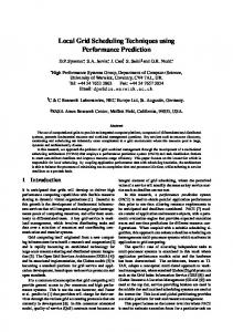
Example 1.6 (The Family of Shop Scheduling problems) The class of shop scheduling problem is characterized by a fixed subdivision of a task into subtasks. The subtasks are a priori determined in terms of their number and duration. In the shop scheduling settings, the whole coarse-grain task is called job, and is compound of a totally ordered set of operations. For this problem family, each operation is atomic, whereas a job can be preempted. Noticeable instances of this class of problems are Job-Shop, Flow-Shop and Open-Shop scheduling, outlined in the following. The Job-Shop Scheduling problem just consists in an instantiation of the scheduling problem within the shop environment. The only difference is that the compatibility matrix has only one non-zero entry for each task, i.e., a task must be assigned to a single and given processor. The Flow-Shop problem differs from Job-Shop by the fact that we schedule the jobs in a pipeline. That is, the processors are arranged in a ordered sequence, and each job should be completed on a given processor before being assigned to the next one. Finally, in the Open-Shop problem the precedence relation is dropped. Specifically, neither the order of jobs, nor the order of the tasks within each job are determined. In Figure 1.2 we report an example of a solution for a generic shop scheduling problem, represented as a processor schedule Gantt chart. This kind of schedule visualization is quite common in practice.

processors

10

1. Introduction to Scheduling Problems

σ( t 12) p1

t 21

t 12

t 32

j j

p

2

t

t

31

t

22

j

13

1

2

3

τ( t ) 23

p

3

t

11

t

t

23

makespan

σ( t 33)

33

time

Figure 1.2: A Gantt chart representation of a schedule for a Shop scheduling problem The diagram should be read as follows. The X axis represents the time scale and each time slot is delimited by means of vertical dashed lines. On the Y axis are reported the processors schedules, each on a separate row. On each row there are a set of bars that represent the set of tasks scheduled on that processor. Each bar spans for a variable length, which is equal to the length of the task. The arrangement of the tasks on a processor line is made accordingly to their starting times σ. As a final remark, we want to emphasize that in this thesis we deal with deterministic scheduling, which means that all the entities of the scheduling problem are known in advance. Another class of scheduling problems, that is not taken into account in this thesis, is the class of stochastic scheduling. This class of problems is characterized by the presence of uncertainty in some scheduling element. For example, the processing times in some manufacturing environments cannot be completely predicted in advance, but are subject to a probability distribution.

1.5

Timetabling Problems

An interesting subclass of scheduling problems is the category of timetabling problems, which is characterized by the fact that the precedence relation (T , ≺) is empty. This means that, in this case, the problem is to schedule the tasks regardless of their mutual time assignment, but looking only at the constraints for the assignment of resources. Furthermore, in most cases, timetabling problems deal with tasks having unitary length, i.e., each task is uniquely associated to a single time slot. Even the terminology for this problem class reflects these changes. In fact, we refer to events and periods instead of, respectively, tasks and processors. Moreover, the basic kind of resources are usually individuals who have to attend to events. We present now the basic version of the timetabling problem, also known as periods/events timetabling. Definition 1.8 (General Timetabling Problem) Given a set of n events E = {e1 , . . . , en }, a set of m resources R = {r1 , . . . , rm }, a set of p periods P = {1, . . . , p}, and an m × n matrix of resource requirements ρij , the general timetabling problem consists in assigning a period τi to each event ei in such a way that the following conditions are met: (1) no individual resource is required to be present for two or more events at the same time, i.e., τi = τi′ ⇔ ρij 6= ρi′ j (j = 1, . . . , m);

1.5. Timetabling Problems

11

(2) there must be sufficient other resources to service all the events at the times they have been scheduled. The assignment τ is called a timetable. The general timetabling problem can easily be modeled within the already presented Graph Coloring framework. The graph encoding is as follows: each event is associated to a vertex of the graph, and there is an edge between two vertices if they clash, i.e., the events cannot be scheduled in the same period because at least one individual has to attend both of them. Then, periods are regarded as colors, and the scheduling of events to periods is simply a coloring of the graph. Considerable attention has been devoted to automated timetabling during the last forty years. Starting with [67], many papers related to automated timetabling have been published in conference proceedings and journals. In addition, several applications have been developed and employed with good success. Example 1.7 (The family of Educational Timetabling problems) In this thesis we focus on the class of Educational Timetabling problems. These kind of problems consists in scheduling a sequence of events (typically lectures or examinations), involving teachers and students, in a prefixed period of time. The schedule must satisfy a set of constraints of various types, which involve, among others, avoiding the overlap of events with common participants, and not excessing the capacity of rooms. Usually the goal is to obtain solutions that minimize student and teacher’s workload. A large number of variants of Educational Timetabling problems have been proposed in the literature, which differ from each other by the type of events, the kind of institution involved (university or school) and the type and the relative influence of constraints. Noticeable examples of this class of problems are School Timetabling, Course Timetabling and Examination Timetabling. The latter two problems are discussed in detail in the applicative part of the thesis The common ground of these problems is that they all are combinatorial problems (search or optimization ones), are NP -hard, and are subject to similar types of constraints (overlap, availability, capacity, etc.). Additionally, almost all of them have been recognized to be genuinely “difficult on the average” in practical real-life cases. For this reason, such problems have not been addressed in a complete and satisfactory way yet, and are still a matter of theoretical research and experimental investigation.

12

1. Introduction to Scheduling Problems

2 Local Search The simplest way for presenting the intuition behind Local Search is the following: imagine a climber who is ascending a mountain on a foggy day1 . She can view the slope of the terrain close to her, but she cannot see where the top of the mountain is. Hence, her decisions about the way to go must rely only upon the slope information. The climber has to choose a strategy to cope with this situation, and a reasonable idea is, for example, choosing to go uphill at every step until she reaches a peak. However, because of the fog, she will never be sure whether the peak she has reached is the real summit of the mountain, or just a mid-level crest. Interpreting this metaphor within the optimization framework, we can view the mountain as described by the shape of the objective function. The choice among the possible actions for improving the objective function must be made by watching near or local solutions only. Finally, the inherent problem of this kind of search is that, in general, nobody can assure that the best solution found by the Local Search procedure is actually the globally best solution or only a socalled local optimum2 . Local Search is a family of general-purpose techniques for search and optimization problems, that are based on several variants of the simple idea presented above. In a way, each technique prescribes a different strategy for dealing with the foggy situation. The application of Local Search algorithms to optimization problems dates back to early 1960s [48]. Since that time the interest in this subject has considerably grown in the fields of Operations Research, Computer Science and Artificial Intelligence. Local Search algorithms are non-exhaustive in the sense that they do not guarantee to find a feasible (or optimal) solution, but they search non-systematically until a specific stop criterion is satisfied. Nevertheless, these techniques are very appealing because of their effectiveness and their widespread applicability. Some authors also classify other optimization paradigms as belonging to the Local Search family, such as Evolutionary Algorithms and Neural Networks. However, these paradigms are beyond the scope of this thesis and will not be presented. A complete presentation of these topics and their relationships with the Local Search framework is available, e.g., in [2]. In the rest of the chapter we will describe more formally the concepts behind this optimization paradigm, presenting the basic techniques proposed in the literature and some improvements over the basic strategies. Finally we will outline our attempt to systematize the class of composite strategies, based on the employment of more than one definition of proximity.

2.1

Local Search Basics

The basic setting for combinatorial problems presented in Section 1 must be slightly modified in order to take into account the characteristics of Local Search algorithms. To this aim we need to 1 In

any case, we do strongly advise the reader not to climb up mountains during bad weather conditions! in some restricted cases it is possible to prove some results that guarantee the convergence to a global optimum 2 However,

14

2. Local Search

define three entities, namely, the search space, the neighborhood relation, and the cost function. A combinatorial problem upon which these three entities are defined is called a Local Search problem. A given optimization problem can give rise to different Local Search problems for different definitions of these entities. Definition 2.1 (Search Space) Given a combinatorial optimization problem Π, we associate to each instance π of it a search space Sπ , with the following properties. 1) Each element s ∈ Sπ represents an element x ∈ S. 2) At least one optimal element of F is represented in Sπ . If the previous requirements are fulfilled, we say that we have a valid representation or valid formulation of the problem. For simplicity, we will write just S for Sπ when the instance π (and the corresponding problem Π) is clear from the context. Furthermore, we will refer to elements of S as solutions. In general, the search space Sπ and the set of solutions S of a problem are equal, but there are a few cases in which these entities differ. In such case we work on an indirect representation of the search space, and we require that the representation preserves the information about the optimal solutions. For example, for the family of Shop Scheduling problem, a common search space is the permutation of tasks on the different processors. This is an indirect representation of the schedule starting times, under the assumption of dealing with left-justified schedules3 . The encoding clearly preserves the optimal solutions when we are looking at minimizing the makespan. Definition 2.2 (Neighborhood Relation) Given a problem Π, an instance π and a search space S for it, we assign to each element s ∈ S a set N (s) ⊆ S of neighboring solutions of s. The set N (s) is called the neighborhood of s and each member s′ ∈ N (s) is called a neighbor of s. For each s the set N (s) needs not to be listed explicitly. In general it is implicitly defined by referring to a set of possible moves, which define transitions between solutions. Moves are usually defined in an intensional fashion, as local modifications of some part of s. The “locality” of moves (under a correspondingly appropriate definition of distance between solutions) is one of the key ingredients of local search, and actually it has also given the name to the whole search paradigm. Nevertheless, from the definition above there is no implication for the existence of “closeness” among neighbors, and actually complex neighborhood definitions can be used as well. Definition 2.3 (Cost Function) Given a search space S for an instance π of a problem Π, we define a cost function F , which associates to each element s ∈ S a value F (s) that assesses the quality of the solution. In practice, the co-domain of F is a well-founded totally ordered set, like the set of natural numbers or the non-negative reals. The cost function is used to drive the search toward good solutions of the search space and is used to select the move to perform at each step of the search. For search problems, the cost function F is generally based on the so-called distance to feasibility, which accounts for the number of constraints that are violated. For optimization problems, instead, F takes into account also the objective function of the problem. 3 Given a sequence of tasks represented as a permutation, the left-justified schedule is the schedule that comply with the sequence and assigns to each task its earliest possible starting time.

2.2. Local Search Algorithms

15

procedure Local Search(Search Space S, Neighborhood N , Cost Function F ); begin s0 := InitialSolution(S); i := 0; while (¬StopCriterion(si , i)) do begin m := SelectMove(si , F, N ); if (AcceptableMove(m, si , F )) then si+1 := si ◦ m; else si+1 := si ; i := i + 1 end end; Figure 2.1: The abstract local search procedure

In this case, the cost function is typically defined as a weighted sum of the value of the objective function and the distance to feasibility (which accounts for the constraints). Usually, the highest weight is assigned to the constraints, in order to give preference to feasibility over optimality. In some optimization problems, the search space can be defined in such a way that it represents only the feasible solutions. In this case, the cost function generally coincides with the objective function of the problem.

2.2

Local Search Algorithms

According to the abstract procedure reported in Figure 2.1, a Local Search algorithm starts from an initial solution s0 ∈ S, and iterates exploring (or navigating) the search space, using the moves associated with the neighborhood definition. At each step it makes a transition between one solution s to one of its neighbors s′ . When the algorithm makes the transition from s to s′ , we say that the corresponding move m has been accepted, and we also write that s′ is equal to s ◦ m. The selection of moves is based on the values of the cost function. However, the precise way in which this selection takes place depends on the specific Local Search technique, and is explained in the next section. Two important components of any Local Search algorithm are the choice of the initial solution and the stop criterion, which determines when the search phase is over and the best solution found is returned. Regarding the initial solution s0 , for some techniques, e.g., Simulated Annealing (Sect. 2.3.2), its construction is part of the algorithm, and thus it has to be done in a specific way. For other methods, s0 can be freely constructed by some algorithm or generated randomly. The stop criterion is generally part of the specific technique, and it is based either on specific qualities of the solution reached or on a maximum number of iterations. Both issues will be discussed for the specific techniques presented in the following. Notice that all these design issues belong to a higher conceptual level than the basic entities presented before. It is only assumed that a Local Search representation exists, and that it complies with the previously described properties. For this reason, Local Search algorithms are often referred as meta-heuristics, since they do not rely on the specific representation of the underlying problem. Furthermore, the description of the algorithms at an abstract level is an interesting characteristic that we profitably exploited in the design of EasyLocal++, the software tool for Local Search presented in Chapter 8.

16

2. Local Search

Abstract feature InitialSolution SelectMove AcceptableMove

Hill Climbing not specified random non-worsening

StopSearch

idle iterations

Simulated Annealing random random always improving, worsening with probability e−∆/T frozen system

Tabu Search not specified best non tabu always

idle iterations

Table 2.1: Characterization of the Basic Local Search techniques

2.3

Basic Local Search Techniques

Now, we are going to illustrate the three most popular Local Search techniques proposed in the literature: Hill Climbing, Simulated Annealing and Tabu Search. Hill Climbing relies on the basic idea chosen by the climber in the metaphor proposed above: at each step of the search a move that “leads uphill” is performed. Instead, Simulated Annealing and Tabu Search represent two essentially different approaches for improving this simple idea. Specifically, the former relies on probabilistic, memoryless decisions, whereas the latter is based on the use of a memory of previously visited solutions. Hence, the three methods correspond to three different search philosophies: simple, probabilistic-driven, and memory-based. The basic features of the techniques are summarized in Table 2.1; we now provide a more detailed description of them.

2.3.1

Hill Climbing

As mentioned, among Local Search techniques, the simplest ones are based on some forms of Hill Climbing. The term comes from the iterative improvement scheme employed: at each step of the search, a move that either improves the value of the objective function or reduces the distance to feasibility is selected4 . Since there is no common agreement on which is the precise characterization of the “Hill Climbing” techniques, in this thesis we denote with this term the whole family of techniques based on the idea of making only moves that either improve the cost function or leave its value unchanged (the so-called sideway moves). The most well-known form of Hill Climbing is the Steepest Hill Climbing (SHC) technique. At each iteration SHC selects, from the whole neighborhood N (s) of the current solution s, the element s′ = s ◦ m which has the minimum value of the cost function F . The procedure accepts the move m only if it is an improving one. Consequently, the search stops as soon as it reaches a local minimum. As an example, the GSAT procedure proposed in [119] for the solution of the Satisfiability problem is a variant of SHC. The difference stems from the fact that GSAT accepts also sideways moves and breaks ties arbitrarily. Therefore GSAT has the capability of navigating plateaus (i.e., large regions of the search space where the cost function is constant), whereas standard SHC is trapped, considering them as local minima. Another popular Hill Climbing technique is Random Hill Climbing (RHC). This technique selects at random (with or without a uniform probability distribution) one element s′ = s ◦ m of the set N (s) of neighbors of the current solution s. The move m is accepted, and thus s′ becomes the current solution for the next iteration if m improves or leaves equal the cost function, otherwise the solution remains unchanged for the next iteration. One remarkable Hill Climbing technique, which combines features of SHC and RHC, is the MinConflict Hill Climbing (MCHC) of Minton et al. [99]. MCHC is specifically designed for constraint satisfaction problems, and the moves are defined as value changes of one variable according to its domain. 4 Despite its name, this technique is applicable both to minimization and maximization problems. The strategy, in case of minimization problems, is to “descend” the hilly landscape looking for the lowest valley.

2.3. Basic Local Search Techniques

17

In MCHC, the selection of the move is divided into two phases, which are performed using two different strategies. Specifically, MCHC first looks randomly for one variable v of the current solution s that is involved in at least one constraint violation. Subsequently, it selects among the moves in N (s) that change only the value of v, the one that creates the minimum number of violations (arbitrarily breaking ties). Other forms of Hill Climbing, like for example the Fast Local Search technique of Tsang and Voudouris [129], can be regarded as improvements of the ones already presented. However, a complete discussion of these techniques falls beyond the scope of this thesis. Both RHC and MCHC accept the selected move if and only if the cost function value is improved or is left at the same value. Therefore, like GSAT, they navigate plateaus, but are trapped by strict local minima. Different stop criteria have been used for Hill Climbing procedures. The simplest one is based on the total number of iterations: the search is stopped when a predetermined number of steps has been performed. An improved version of this criterion is based on the number of iterations without improving the cost function value of the best solution found so far. This way, search trials that are exploring promising paths are let to run longer than those that are stuck in regions without good solutions. Other ad hoc early termination procedures are generally used such as stopping the iteration process if the cost function has crossed a certain value. In principle, Hill Climbing procedures could also stop when they reach a strict local minimum (i.e., a solution whose neighborhood is made up of solutions having greater cost). Unfortunately, though, in general they cannot recognize such a situation.

2.3.2

Simulated Annealing

Simulated Annealing was proposed by Kirkpatrick et al. [83] and Cerny [29] and extensively studied by Aarts and Korst [3], van Laarhoven and Aarts [132] among other researchers. The method got that name after an analogy with a simulated controlled cooling of a collection of hot vibrating atoms. The idea is based on accepting non-improving moves with probability that decreases with time. The process starts by creating a random initial solution s0 . The main procedure consists of a loop that randomly generates at each iteration a neighbor of the current solution. Given a move m, we denote with ∆ the difference in the cost function between the new solution and the current one, i.e., ∆ = f (s ◦ m) − f (s). If ∆ ≤ 0 the new solution is accepted and becomes the current one. Conversely, if ∆ > 0 the new solution is accepted with probability e−∆/T , where T is a parameter, called the temperature. The temperature T is initially set to an appropriately high value T0 . After a fixed number of iterations, the temperature is decreased by the cooling rate α, so that at each cooling step n, Tn = α × Tn−1 . In general α is in the range 0.8 < α < 1. The procedure stops when the temperature reaches a low-temperature region, that is when no solution that increases the cost function is accepted anymore. In this case we say that the system is frozen. Note that for “low temperatures” the procedure reduces to an RHC, therefore the final state obtained by Simulated Annealing will clearly be a local optimum. The control parameters of the procedure are the cooling rate α, the number of moves sampled at each temperature n, and the starting temperature T0 . Since the state change in the Simulated Annealing depends only on the previous state and in a randomly drawn transition, the behavior of the algorithm can be modeled and analyzed by means of Markov Chains [1]. Under the hypotheses of stationary distribution, it is possible to assure the asymptotic convergence of this technique to a global optimum Among others, we remark the works of Johnson et al. [76, 77] on this subject. They discuss in detail the application of Simulated Annealing to a wide range of optimization problems and the impact of different design choices in the performance of the algorithms. The one presented above is the most common form of Simulated Annealing. Nevertheless, many variants of this scheme have been proposed for Simulated Annealing. For example, the way the

18

2. Local Search

temperature is decreased, i.e. the cooling schedule, can be different from the one mentioned above, which is called geometric and is based on the parameter α. For example, two other cooling schemes, called polynomial and efficient are described in [1]. We do not discuss them in detail, but we just mention that they introduce a very limited form of memory. In fact, they are both based on monitoring the quality of the solutions visited at the given temperature Tn , and choosing the new temperature accordingly. Specifically, in the polynomial scheme, the new temperature Tn+1 is chosen on the basis of the standard deviation of the cost function in all solutions at temperature Tn . Similarly, in the efficient scheme, Tn+1 is based on the number of accepted moves at temperature Tn . Another kind of schedule, called adaptive [49], allows also of reheating the system, depending on some statistics of the cost function (mainly the standard deviation of the cost changes).

2.3.3

Tabu Search

Tabu Search was proposed by Glover [60–62] in the late 1980s, and since then it has been employed by many researchers for solving problems in different domains [28, 33, 37, 59, 64, 70, 112]. As sketched in the beginning of Section 2.3, Tabu Search is a method in which a fundamental role is played by keeping track of features of previously visited solutions. We discuss in this section only a basic version of Tabu Search, which makes use of memory in a limited way. Some more complex features will be briefly discussed at the end of the Section, but for an exhaustive treatment of Tabu Search we refer to the recent, comprehensive book on the topic [65]. The basic mechanism of Tabu Search is quite simple: at each iteration a subset Q ⊆ N (s) of the neighborhood of the current solution s is explored. The member of Q that gives the minimum value of the cost function becomes the new current solution independently of the fact that its value is better or worse than the value of s. To prevent cycling, there is a so-called tabu list, i.e., a list of moves that are forbidden to be performed. The tabu list comprises the last k moves, where k is a parameter of the method, and it is run as a queue; that is, whenever a new move is accepted as the new current solution, the oldest one is discarded. Notice that moves, not solutions, are asserted to be tabu. Therefore, a move m can be tabu even if, when applied to the current solution s, it leads to an unvisited solution. In other words, the basic Tabu Search scheme avoids visiting not only previous solutions, but also solutions that share features with the already visited ones. This mechanism prevents cycling, but in its simple form it can overlook good solutions. For this reason, there is also a mechanism called aspiration criterion that overrides the tabu status of a move: if in a solution s a move m gives a large improvement of the cost function, the solution s ◦ m is accepted as the new current one regardless of its tabu status. More precisely, this mechanism makes use of an aspiration function A. For each value t of the cost function, A computes the cost value that the algorithm aspires to reach starting from t. Given a current solution s, the cost function F , and the best neighbor solution s′ ∈ Q, if F (s′ ) ≤ A(F (s)), then s′ becomes the new current solution, even if the move m that leads to s′ has a tabu status. However, other kinds of aspiration functions, not generally related to the cost function, are also considered in some implementations. In some proposals, it is not the move itself but rather some attributes of it to be considered tabu. The attributes that make a move tabu are generally known as tabu-active ones. The choice of the tabu-active attributes are obviously dependent on the specific problem. The Tabu Search procedure stops either when the number of iterations reaches a given value or when the value of the cost function in the current solution reaches a given lower bound. The main control parameters of the basic Tabu Search procedure are: the length of the tabu list, the aspiration function A, and the cardinality and definition of the set Q of neighbor solutions tested at each iteration. Notice that the tabu list needs not to be physically implemented as a list. More sophisticated data structures can be used to improve the efficiency of checking the tabu status of a move. For example, some hashing mechanisms are used in [142].

2.4. Improvements on the Basic Techniques

19

One of the key issues of Tabu Search is the tabu tenure mechanism, i.e., the way in which we fix the number of iterations that a move should be considered as tabu. The basic mechanism described above, which is based on the fixed-length tabu list, has been refined and improved by several authors with the purpose of increasing the robustness of the algorithms. A first improvement, proposed by Taillard [124] and commonly accepted, is the employment of a tabu list of variable size. Specifically, the size of the tabu list is kept at a given value for a fixed number of iterations, and then it is changed. For setting the new length, there is a set of candidate lengths, and they are used circularly. A further improvement of this idea is the one proposed by Gendreau et al. [59]: each performed move is inserted in the tabu list together with the number of iterations tabu iter that it is going to be kept in the list. The number tabu iter is randomly selected between two given parameters tmin and tmax (with tmin ≤ tmax ). Each time a new move is inserted in the list, the value tabu iter of all the moves in the list is updated (i.e. decremented), and when it gets to 0, the move is removed. More complex prohibition mechanisms are based on some form of long term memory. For example in the frequency based tabu list a table of frequencies of accepted moves is maintained and a move is regarded as tabu if its frequency is greater than a given threshold. This way, cycles whose length is greater than the tabu list can be prevented. Regarding the aspiration function, we have mentioned that several criteria have been proposed in the literature. The most common one is the following: if a move leads to a solution that is better than the current best solution found so far, it is accepted even if it is tabu. In other words, assuming s∗ is the current best solution, the aspiration function A is such that A(F (s)) = F (s∗ )− ǫ for all s. In some cases, the aspiration mechanism is used to protect the search from the possibility that in a given state all moves are tabu. In such cases, the aspiration function is set in such a way that at least one move fulfills its criterion, and its tabu status is removed. In other cases, the aspiration mechanism is set in such a way that, if a move with a big impact on the solution is performed, the tabu status of other lower-influence moves is dropped. The underlying idea is that after a big change, the effect of moves has changed completely, therefore there is no reason to keep them tabu. Other types of aspiration functions are defined in [65].

2.4

Improvements on the Basic Techniques

One of the main issues of local search techniques is the way they deal with the local minima of the cost function. Even if the search procedure employs some specific mechanism for escaping them (like Simulated Annealing or Tabu Search), a local minimum still behaves as a sort of attractor. Intuitively, when a trajectory moves away from a local minimum, it steps through a set of “near” solutions. Therefore, even though it is not allowed to go back to the minimum itself, the trajectory still tends to stay in the region where the local minimum is located, instead of moving toward a “farther” region 5 . For this reason, the search procedure needs to use some form of diversification strategy that allows the search trajectories not only to escape a local minimum, but to move “far away” from it, in order to avoid this sort of chaotic trapping around the local minimum. However, for practical problems the objective function is usually correlated in neighbors (and near) solutions. Therefore, once a good solution is found, it is reasonable to search in its proximity to find a better one. For this reason, when a local minimum is reached the search should be in some way intensified around it. In conclusion, the search algorithm should be able to balance the two conflicting objectives: it should diversify and intensify by moving outside the attraction area of already visited local minima, but not too far from it. Several strategies have been proposed in the literature to solve this issue by giving the appropriate quantity of intensification and diversification in different phases of the search (see [65]). 5 We remark that here the quoted terms are used in an intuitive way, without referring to any metric or distance. A more formal discussion is given, for example, in [8].

20

2. Local Search

One example of such a strategy is the shifting penalty (see, e.g., [59]), which is a mechanism that changes continuously the shape of the cost function in an adaptive manner. This way, it causes the local search algorithm to visit solutions that have a different structure than the previously visited ones. In detail, the constraints which are satisfied for a given number of iterations will be relaxed in order to allow the exploration of solutions where those constraints do not hold. Conversely, if some constraint is not satisfied for a long time, it is tightened, with the aim of driving the search toward its satisfaction. Another control knob that can be used specifically for the Tabu Search technique is the length of the tabu list. The dynamic tabu list approach adaptively modifies the tabu list length in the following way: if the sequence of the last performed moves is improving the cost function, then the tabu list length is shortened to intensify the search; otherwise, if a sequence of moves induces a degradation, the length of the tabu list is extended to escape from that region of the search space. As it has already been noticed, Local Search meta-heuristics belong to an abstract level with respect to the underlying Local Search problem. For this reason, Local Search techniques can be easily composed and hybridized with other methods. In addition, the Local Search paradigm can be regarded as a useful laboratory for the study of learning mechanisms, which can bias the search toward more promising regions of the search space. In the following we present some attempts to investigate the proposed issues presented in the literature.

2.5

Local Search & Learning

One characteristic of some Local Search techniques, namely Hill Climbing and Simulated Annealing, is the fact that they are completely oblivious. That is, they do not maintain any information about the past history of the search. Only a limited form of memory is used in Tabu Search through the tabu list mechanism, which preserves track of the last performed moves. On the contrary, it is a common intuition that during search there is a lot of additional information, gathered from the trajectory followed and from the evaluations made, that could be learned. Such information could then be used at a later stage of the search. For example, as claimed by Battiti in [8], it should be possible to learn, with a reasonable overhead of computational time, some parts of the objective function landscape 6 in order to improve search effectiveness. This information can be used either to tune on-line the search parameters (e.g., the tabu list length) or to model the cost function and/or the neighborhood relation. We refer to this kind of learning as adaptive learning, because at each step of the search some components are modified or adapted in order to take into account the new information. In this kind of learning, the search space becomes a search environment. The learning mechanism basically collects features from the environment and reacts upon them (for example in a reinforcement learning fashion [81]). An example of this kind of techniques is the Guided Local Search (GLS) [137]. GLS uses an augmented cost function, which includes a component that takes care of solution features. This component is adaptively modified during the search, according to a given set of modification actions. An alternative approach of learning is what we call predictive learning. In [11], Boyan and Moore propose an algorithm called STAGE. This technique learns to predict the outcome of a search as a function of state features along a search trajectory. The algorithm relies on the exploitation of statistical models of the features built during the search, considering the search as a Markov Decision Process. The prediction is then used for modifying the cost function for the purpose of biasing search trajectories toward better optima. 6 With

this term we intend the plot of the cost function over the variable assignments.

2.6. Composite Local Search

2.6

21

Composite Local Search

One of the attractive properties of the Local Search paradigm is that different techniques can be combined and alternated to give rise to complex algorithms. Several approaches of combination have been proposed over the years; for example, the effectiveness of alternating two Local Search algorithms, called tandem search, has been stressed by several authors (see, e.g., [65]). Specifically, when one of the two algorithms (usually the second one) is not used with the aim of improving the cost function, but rather for diversifying the search region, this pattern is called Iterated Local Search (see, e.g., [123]). In this case the second algorithm is normally called the mutation operator or the kick move. Another example of composition of basic techniques is the WalkSAT algorithm for the Satisfiability problem [118]. It alternates a Local Search phase with a random perturbation phase (called random walk, hence the name of the technique) that is used to escape the local optimum and to start again the search in a new region of the search space. A completely different yet relatively unexplored approach relies on the change of neighborhood during the search. Hansen and Mladenovi´c recently propose what they called Variable Neighborhood Search (VNS) [68]. Differently from other meta-heuristics, VNS does not follow a trajectory but explores increasingly distant neighborhoods of the current solution (where the distance is related to some metric that induces a neighborhood). When an improvement in the cost function is found (regardless of the distance), the new solution becomes the starting point for the new search step. In some sense the family of neighborhoods acts as macro moves in the classical Local Search setting, and describes a family of methods. Furthermore, VNS is independent of the particular meta-heuristic employed and therefore can be coupled with different techniques.

Multi-Neighborhood Search The aforementioned approaches can be neatly classified according to the level of granularity they belong to. In fact, both the tandem and the WalkSAT approaches aim at combining whole algorithms (either directly based on Local Search or not), whereas the VNS strategy deals with neighborhood combination at a finer level of granularity. In our recent work we attempt to systematize these ideas in a common framework. In [42] we propose a set of operators for combining neighborhoods and algorithms that generalizes the aforementioned techniques. We name this approach Multi-Neighborhood Local Search and we will present it in detail in Chapter 3. Moreover, we exemplify its use in the solution of various scheduling problems throughout this thesis. The idea behind Multi-Neighborhood Search is to define a set of operators for combining neighborhoods (namely the neighborhood union and the neighborhood composition) and basic techniques based on different neighborhoods (what we call token-ring search). Furthermore, with these operators it is possible to define additional Local Search components that we call kickers which deal with perturbation in the spirit of random walks of the WalkSAT algorithm.

2.7

Hybrid Techniques

As mentioned earlier, the Local Search techniques can be profitably hybridized with other methods, giving rise to more powerful solving strategies. Even though Local Search has been successfully combined with other incomplete methods, such as Genetic Algorithms, in this section we restrict our attention to the employment of Local Search in joint action with the class of constructive methods and dealing with partial solutions.

2.7.1

Local Search & Constructive methods

There is a variety of techniques for combinatorial optimization problems which are based on the use in tandem of a constructive method followed by a Local Search step.

22

2. Local Search

For example, Yoshikawa et al. [143] combine a sophisticated greedy algorithm, called ReallyFully-Lookahead, for finding the initial solution and a Local Search procedure for the optimization phase. The Local Search algorithm employed is the Min-Conflict Hill-Climbing (MCHC), defined by Minton et al. [99]. In [122], Solotorevsky et al. employ a propose-and-revise rule-based approach to the Course Timetabling problem. The solution is built by means of the Assignment Rules. When the construction reaches a dead-end, the so-called Local Change Rules come into play so as to find a possible assignment for the unscheduled activity. However, the authors only perform a single step before restarting the construction, and their aim is only to accommodate the pending activity, without any look-ahead mechanism. Other researchers, like Feo and Resende in the GRASP procedure [50], propose an iterative scheme that uses the propose-and-revise approach as an inner loop. Starting with a constructive method, a Local Search scheme is later applied. Some kind of adaptation will guide the constructive phase to a new attempt that again will be followed by a local-search step. Glover et al. [63] present an adaptive depth-first search procedure that combines elements of Tabu Search and Branch & Bound for the solution of the min-Graph Coloring problem. They build an initial solution through a greedy heuristic (called DANGER), and then they try to improve it using Tabu Search to control the backtracking mechanism. The Tabu Search phase prevents the algorithm to fall in already visited local optima by imposing additional backtracking steps. In the algorithm the “degree” of Local Search may be controlled by a parameter that ranges from a pure Branch & Bound algorithm to a pure Tabu Search one.

2.7.2

Local Search on Partial Solutions

In [113] Schaerf proposes a more complex way of combining (backtracking-free) constructive methods and Local Search techniques. The technique incrementally constructs the solution, performing a Local Search run each time the construction reaches a dead-end. Local Search is therefore performed on the space of partial solutions and is guided by a cost function based on three components: the distance to feasibility of the partial solution, a look-ahead factor, and (for optimization problems) a lower bound of the objective function. In order to improve search effectiveness, this technique makes use of an adaptive relaxation of constraints and an interleaving of different look-ahead factors. The technique has been successfully applied on two real-life problems: university course scheduling and sport tournament scheduling. A variant of this technique, called Generalized Local Search, is used in [116] for the solution of the employee timetabling problem. Another approach was employed in [144] where the authors combine constructive and Local Search methods in a different way. Their method finds a partial solution using Local Search, and then explores all its possible completions using a backtracking-based algorithm. Therefore, the authors also make use of Local Search on partial solutions, but they have no notion similar to the look-ahead factor in [113].

3 Multi-Neighborhood Search One of the most critical features of Local Search is the definition of the neighborhood structure. In fact, for most popular problems, many different neighborhoods have been considered and experimented. For example, at least ten different kinds of neighborhood have appeared in the literature for the Job-Shop Scheduling problem (see [131] for a recent review). Moreover, for most common problems, there is more than one neighborhood structure that is sufficiently natural and intuitive to deserve systematic investigation. We believe that the exploitation of different neighborhood structures, or even different metaheuristics, in a compound Local Search strategy can improve the results with respect to the algorithms that use only a single structure or technique. An evidence of this conjecture is provided in Section 9.6.2, where we present the results of a compound strategy for the Graph Coloring problem. Even though in that experiment we employ a single neighborhood function, we show that the use of more than one Local Search technique in a compound strategy outperforms the basic algorithms. The main motivation for considering combination of diverse neighborhoods is related to the diversification of search needed to escape from local minima. In fact a solution that is a local minimum for a given neighborhood definition, is not necessarily a local minimum for another one. For this reason, an algorithm that uses both has more chances to move toward better solutions. More generally, the use of different neighborhoods may lead to trajectories that make the overall search more effective. However, so far little effort has been devoted to the combination of more than one neighborhood function inside a single Local Search algorithm (see Section 2.6). In our recent work [38, 42] we attempted to overcome this lack and we have formally defined and investigated some ways to combine different neighborhoods and algorithms. We defined a set of operators that automatically compound basic neighborhoods, and a solving strategy that combines several algorithms, possibly based on different neighborhoods. We named this approach Multi-Neighborhood Search. In this chapter we provide a formal description of the Multi-Neighborhood Search framework and we describe its use in the solution of an actual scheduling problem, namely the Course Timetabling problem.

3.1

Multi-Neighborhood Operators

Consider an instance π of a search or optimization problem Π, a search space S for it and a set k of neighborhood functions N1 , . . . , Nk defined on S. The functions Ni are obviously problem-dependent, and are defined by the person who investigates the problem. Though there are many ways to combine different neighborhoods, in this work we formally define and investigate the following three: Neighborhood union: we consider as compound neighborhood the union of many neighborhoods in the set-theoretical sense. The Local Search algorithms based on this neighborhood select, at each iteration, a move belonging to any of the components.

24

3. Multi-Neighborhood Search

N (s i ) 2

si

si N (s i )

N (s i )

1

1

N (s i ) 2

Figure 3.1: Neighborhood Union Neighborhood composition: the neighborhood is composed of chains of moves belonging to different neighborhoods. The types of the moves in the chain are fixed, and are based on the order of composition. Neighborhood total composition: is a more general case of neighborhood union and composition. As with the composition operator, the atomic moves are chains of moves. However, in this case, the moves in the chain can belong to any of the neighborhoods employed, regardless of the order of composition. In order to define these operators we have to prescribe how the elements of the compound neighborhood are generated, starting from the elements of the basic neighborhoods. Additionally, according to the concepts presented in Section 2.2, for providing a valid definition of the compound neighborhoods we need also to define the strategies for their exploration (i.e., the criterion for selecting a random move in the neighborhood and the definition of the move inverse).

3.1.1

Neighborhood Union

We start presenting the most straightforward combination operator, i.e., the neighborhood union. A pictorial representation of this operator is reported in Figure 3.1, whereas its formal definition is as follows. Definition 3.1 (Neighborhood Union) Given k neighborhood functions N1 , . . . , Nk , we call neighborhood union, written N1 ⊕ · · · ⊕ Nk , the neighborhood function such that, for each state s, the set N1 ⊕ · · · ⊕ Nk (s) is equal to N1 (s) ∪ · · · ∪ Nk (s). A member of this neighborhood is simply a move m ∈ Ni for a suitable index i. A random element in the neighborhood union N1 ⊕ · · · ⊕ Nk is selected at random from any of the Ni . The thorough exploration of the N1 ⊕ · · · ⊕ Nk is performed by exhaustively exploring each Ni and selecting the overall best solution. The definition of inverse of a move, related to the prohibition mechanism of Tabu Search, is the following. Given a move m ∈ N1 ⊕ · · · ⊕ Nk , we have that m ∈ Ni for a suitable index i. If we denote with m−1 the inverse of m in Ni , we consider the move m−1 as inverse also in the i i compound neighborhood N1 ⊕ · · · ⊕ Nk . Notice that, in this case, the order of the neighborhoods in the combination is not relevant and it is not worth to repeat the same neighborhood more than once, since the set union is an associative, commutative and idempotent operator. Furthermore, according to this definition, there are several possible choices for the selection of a random move in the neighborhood union. In fact, the simplest random distribution for selecting a move in N1 ⊕ · · · ⊕ Nk from a state s first selects uniformly a random i (with 1 ≤ i ≤ k), and then selects a random state s′ ∈ Ni (s) as to the random distribution associated with Ni . In this case, the selection in the neighborhood union is not uniform, because it is not weighted based on the cardinality of the sets Ni (s). However, this strategy could be unsatisfactory for some applications. In such cases the random distribution for selecting the neighborhood can change by taking into account also the size of each

3.1. Multi-Neighborhood Operators

25

N (s i ) 2

si N (s i ) 1

si

N (s i ) 1

N (s i ) 2

Figure 3.2: Neighborhood Composition neighborhood that take part in the union.

3.1.2

Neighborhood Composition

Now we move to neighborhood composition, depicted in Figure 3.2. The formal definition of the operator is as follows. Definition 3.2 (Neighborhood Composition) Given k neighborhood functions N1 , . . . , Nk , we call neighborhood composition, denoted by N1 ⊗ · · · ⊗ Nk , the neighborhood function defined as follows. Given two states sa and sb , then sb belongs to N1 ⊗ · · · ⊗ Nk (sa ) if there exist k − 1 states s1 , . . . sk−1 such that s1 ∈ N1 (sa ), s2 ∈ N2 (s1 ), . . . , and sb ∈ Nk (sk−1 ). Intuitively, a composite move is an ordered sequence of moves belonging to the component neighborhoods, i.e., m = m1 m2 . . . mk with mi ∈ Ni . The strategy for selecting a random move in the compound neighborhood N1 ⊗· · ·⊗Nk consists in drawing a random move mi for each component neighborhood Ni (1 ≤ i ≤ k). The complete exploration of the neighborhood is obtained by exploring in inverse lexicographic ordering each component neighborhood Ni . In other words, given a move m = m1 m2 . . . mj . . . mk its successor is m′ = m1 m2 . . . m′j . . . mk , where m′j is the successor of mj in the exploration of the neighborhood Nj (for all 1 ≤ j ≤ k). Concerning the definition of inverse, given a move m = m1 m2 . . . mk belonging to the composite neighborhood N1 ⊗ · · · ⊗ Nk we forbid all the moves m′ = m′1 m′2 . . . m′k such that m′i = m−1 for i some i = 1, . . . , k. It is worth noticing that, differently from the union operator, the order of the Ni for composition is relevant, therefore it is meaningful to repeat the same Ni in the composition.

3.1.3

Total Neighborhood Composition

The total neighborhood composition generalizes both the concepts of neighborhood union and neighborhood composition presented above. A pictorial view of the operator is in Figure 3.3, whereas the formal definition of total neighborhood composition is as follows. Definition 3.3 (Total Neighborhood Composition)

26

3. Multi-Neighborhood Search

N (s i ) 2

si N (s i ) 1

si

N (s i ), N (s i )

2

1

2

Figure 3.3: Total Neighborhood Composition Given k neighborhoods functions N1 , . . . , Nk , and an integer h, we call total neighborhood composition of step h the union of h possible compositions (also with repetitions) of all k neighborhoods. We denote a total composition by ⊙h N1 , . . . , Nk . A move in this neighborhood is an ordered sequence of h moves m1 m2 . . . mh such that mi ∈ N1 ⊕ · · · ⊕ Nk . A random move in the total composite neighborhood can be drawn by picking a random move in the union N1 ⊕ · · · ⊕ Nk for each element mi (1 ≤ i ≤ h) of the move sequence. As in the case of simple neighborhood composition, the exhaustive exploration of the total composite neighborhood is performed by exploring in inverse lexicographic ordering the whole union neighborhood for each move mi (1 ≤ i ≤ h) in the sequence. The inverse of a move m = m1 m2 . . . mh that belongs to a total composition ⊙h N1 , . . . , Nk is the sequence of inverses of the h constituent moves taken in the reverse order, that is m−1 = −1 −1 m−1 h . . . m2 m 1 .

3.2

Multi-Neighborhood Solving Strategies

So far we have presented some operators that combine sets of base neighborhoods in order to build a new composite neighborhood. Then, the resulting neighborhood can be plugged into any metaheuristic giving rise to one complete Local Search algorithm. However, at a higher abstraction level, it is possible also to combine whole algorithms that make use of different neighborhood functions. Consider again a set k of neighborhood functions N1 , . . . , Nk defined on a search space S. Given also a set of n Local Search techniques, we can define k × n different search algorithms ti , called searcher s, by providing each technique with any neighborhood function. A searcher can either be a basic Local Search technique (e.g., Hill Climbing, Simulated Annealing, etc.) or a special purpose Local Search component used for intensification or diversification (like the Kickers presented below). In the following, the searchers based on a basic Local Search algorithm are called runners. A solving strategy controls the search of a set of searchers ti . For example, such a strategy prescribes in which order the algorithms ti should be activated, or under which conditions to accept their outcomes, and so on. This concept corresponds the notion of solver in the EasyLocal++ framework (see Section 8.1.5). In this thesis we experimented only with a simple solving strategy, which turned out to be very effective in the solution of practical problems. The strategy is named token-ring search and is

3.3. Multi-Neighborhood Kickers

27

t1 t2

s0

t3

t1 t2

Search Space

t3

sn

Figure 3.4: Token-Ring Search presented below.

3.2.1

Token-Ring Search

The token-ring search is a sequential solving strategy for combining Local Search algorithms, possibly based on different neighborhood functions. Given an initial state and a set of algorithms, the token-ring search makes circularly a run of each algorithm, always starting from the best solution found by the previous one. An illustration of token-ring search is provided in Figure 3.4, while the formal definition of token-ring search is as follows. Definition 3.4 (Token-Ring Search) Given an initial state s0 , and a set of q searchers t1 , . . . , tq (possibly based on different neighborhood functions), the token-ring search, denoted by t1 ⊲ · · · ⊲ tq , makes circularly a run of all ti . Each searcher ti always starts from the final solution of the previous searcher ti−1 (or tq if i = 1). The token-ring search keeps track of the global best state, and it stops when performs a fixed number of rounds without an improvement of this global best. Each component searcher ti stops according to its own specific criterion. Many specific cases of the general idea of the token-ring strategy have been studied in the literature. For example, Hansen and Mladenovi´c [68] explore the case in which each searcher ti adopts a neighborhood of size larger than ti−1 . The effectiveness of token-ring search for two searchers has been stressed by several authors (see [65]). For example, the alternation of a Tabu Search using a small neighborhood with Hill Climbing using a larger neighborhood has been used by Schaerf [112] for the high-school timetabling problem. Specifically, when one of the two searchers, say t2 , is not used with the aim of improving the cost function, but rather for diversifying the search region, this idea falls under the name of Iterated Local Search (see, e.g., [123]). In this case the run with t2 is normally called the mutation operator or the kick move.

3.3

Multi-Neighborhood Kickers

As stressed by several authors (see, e.g., [93]), local search can benefit from alternating regular runs with some perturbations that allow the search to escape from the attraction area of a local minimum.

28

3. Multi-Neighborhood Search

Kick

s1 Synergic moves

s0 Figure 3.5: Kicks In the Multi-Neighborhood settings, we define a form of perturbation, that we name kick, in terms of neighborhood compositions. A kicker is a special-purpose searcher that makes just one single move, and uses a neighborhood composition (total or simple) of a relatively long length. A kicker can perform either a random kick, i.e., a random sequence of moves, or a best kick, which means an exhaustive exploration of the composite neighborhood searching for the best sequence. Random kicks roughly correspond to the notion of random walk used in [118]. The notion of best kicks is based on the idea of ejection chains (see, e.g., [109]), and generalizes this concept to generic chains of moves (from different neighborhoods). Experiments with kickers as part of a token-ring search, called Run & Kick, are shown in our case study (Chapter 4), and, as highlighted in Section 4.5, the use of best kicks turned out to be very effective in our test instances. Notice that the cardinality of a composition is the product of the cardinalities of all the base neighborhoods, therefore if the base neighborhoods have some few thousand members, the computation of the best kick for a composition of length 3 or more is normally intractable. In order to reduce this complexity, we introduce the problem-dependent notion of synergic moves. For every pair of neighborhood functions N1 and N2 , the user might define a set of constraints that specifies whether two moves m1 and m2 , in N1 and N2 respectively, are synergic or not. This relationship is typically based on equality constraints of some variables that represent the move features. If no constraint is added, the kicker assumes that all moves are synergic. The concept of synergy is illustrated in Figure 3.5. A move sequence belonging to the neighborhood composition is evaluated only if all pairs of adjacent moves are synergic. The intuition behind this idea is that a combination of moves, which are not all focused on the same features of the current state s, have little chance to produce improvements. In that case, in fact, the improvements would have been found by one of the runners that make one step at the time. Conversely, a good sequence of “coordinated” moves can be easily overlooked by a runner based on a simple neighborhood function. In order to build kicks, i.e., chains of synergic moves, the kicker employs a constraint-based backtracking algorithm that builds it starting from the current state s, along the lines presented in [108]. Differently from [108], however, all variables describing a move are instantiated simultaneously, and backtracking takes places only at “move granularity” rather that at the level of each individual variable. That is, the algorithm backtracks at level i if the current move mi has no synergic move in the neighborhood Ni+1 that is feasible if applied in the state reached from s executing the moves of the partial sequence built up to level i. Different definition of synergy are possible for a given problem but, in general, there is a tradeoff between the time necessary to explore the neighborhood and the probability to find good moves. In the case study reported in Chapter 4, we experiment with two different definitions of synergy and compare their results. The reader may wonder why the seemingly computationally expensive random kicks improve over a simple restart from a random initial position. An intuitive reason of this behavior is that a multi-start strategy always restarts from scratch, throwing away possibly useful information gathered during the search (not only the state reached so far but, for example, also the memory employed in the tabu search algorithm). By contrast, the random kicks introduce only some local

3.4. Discussion

29

perturbations and have more chance to retain good solution qualities.

3.4

Discussion

We presented a novel approach for combining different neighborhoods for a given Local Search problem, that generalizes previous ideas presented in the literature. The Multi-Neighborhood Search framework is based on a set of operators for neighborhood combination and in a solving strategy that interleaves basic algorithms possibly equipped with different neighborhood structures. Furthermore we define a Local Search component, called kicker, that is meant to implement a sort of perturbation mechanism based on neighborhood composition. The benefits of the proposed approach resides in the complete generality of our neighborhood operators, in the sense that, given the basic neighborhood functions, the synthesis of the proposed algorithms requires only the definition of the synergy constraint, but no further domain knowledge. Furthermore, as mentioned above, with respect to other Multi-Neighborhood meta-heuristics, such as Variable Neighborhood Search [68] and Iterated Local Search [93], we have tried to give a more general picture in which these previous (successful) proposals fit naturally. Our software tool presented in Chapter 8, generates automatically the code for exploration of composite neighborhood starting from the code for the basic ones. This is very important, from the practical point of view, so that the test for composite techniques is very inexpensive not only in terms of design efforts, but also it terms of human programming resources. In the remaining of the thesis we will extensively use the operators and the strategies presented in this chapter.

30

3. Multi-Neighborhood Search

II Applications

4 Course Timetabling: a Case Study in Multi-Neighborhood Search The university Course Timetabling problem consists in the weekly scheduling of a set of lectures for several university courses within a given number of rooms and time periods. There are various formulations of Course Timetabling (see, e.g., [114]), which differ from each other mostly for the (hard) constraints and the objectives (or soft constraints) they consider. Constraints mainly concern the overlapping of lectures belonging to the same curriculum (i.e., that have students in common), and the simultaneous assignment of more than one lecture to the same room. Objectives are related to the aim of obtaining a compact schedule of lectures belonging to the same curriculum, and to the conflicting goal of spreading the lectures of the same course in a minimum number of days. In this chapter we present an investigation of Multi-Neighborhood Search methods (see Chapter 3) in the domain of Course Timetabling. For the sake of generality, in this work we consider a basic version of the problem. We consider this study as a first step toward a full understanding of the capabilities of MultiNeighborhood techniques.

4.1

Problem Statement

The Course Timetabling problem is a specialization of the general timetabling problem presented in Section 1.5. Now we provide a more formal statement of the problem describing the entities involved and the constraints to be satisfied. Definition 4.1 (The Course Timetabling problem) There are given a set of q courses, C = {c1 , . . . , cq }, a set of p periods, P = {1, . . . , p}, and a set of m rooms, R = {r1 , . . . , rm }: each course ci consists of li lectures to be scheduled in distinct time periods, and is attended by si students. Each room rj has a capacity capj , expressed in terms of number of seats. There are also n groups of courses, G1 , . . . , Gn called curricula, such that any pair of courses belonging to a curriculum Gi have students in common. The output of the problem is an integer-valued q × p matrix T , such that Tik = j (with 1 ≤ j ≤ m) means that course ci has a lecture in room rj at period k, and Tik = 0 means that course ci has no class in period k. We search for the matrix T such that the following hard constraints are satisfied, and the violations of the soft ones are minimized1 : (1) Lectures (hard): The number of lectures of course ci must be exactly li . 1 Hard constraints must be always satisfied in the final solution of the problem. Conversely, soft constraints can be violated, but at the price of deteriorating the solution quality.

34

4. Course Timetabling: a Case Study in Multi-Neighborhood Search

(2) Room Occupancy (hard): Two distinct lectures cannot take place in the same room in the same period. Furthermore, each lecture cannot take place in more than one room. (3) Conflicts (hard): Lectures of courses in the same curriculum must be all scheduled at different times. Similarly, lectures of courses taught by the same teacher must also be scheduled at different times. To the take into account these constraints, we define a conflict matrix CM of size q × q, such that cmij = 1 if there is a clash between the courses ci and cj , cmij = 0 otherwise. (4) Availabilities (hard): Teachers might be not available for some periods. We define an availability matrix A of size q × p, such that aik = 1 if lectures of course ci can be scheduled at period k, aik = 0 otherwise. (5) Room Capacity (soft): The number of students that attend a course must be less than or equal to the number of seats of all the rooms that host its lectures. (6) Minimum working days (soft): The set of periods p is split in w days of p/w periods each (assuming p divisible by w). Each period therefore belongs to a specific week day. The lectures of each course ci must be spread into a minimum number of days di (with di ≤ ki and di ≤ w).

(7) Curriculum compactness (soft): The daily schedule of a curriculum should be as much compact as possible, avoiding gaps between courses. A gap is a free period between two lectures scheduled in the same day and that belong to the same curriculum. Overnight gaps, instead, are allowed. That is, we admit free periods between two courses scheduled in different days. A simpler version of the Course Timetabling problem, that does not involve room assignment, can be easily shown to be NP-hard through a reduction from the k -Graph Coloring problem.

4.2

Search Space, Cost Function and Initial State

In order to solve Course Timetabling by Local Search, first we have to define the basic Local Search entities, namely the search space, the cost function and the strategy for generating the initial solution. Our search space is composed of all the assignment matrices Tik for which the constraints (1) and (4) hold. States for which the hard constraints (2) and (3) do not hold are allowed, but are considerably penalized within the cost function. The cost function is thus a weighted sum of the violations of the aforementioned hard constraints plus the violations of the soft constraints (5) – (7). The weight of constraint type (5) is the number of students without a seat, whereas the weight of constraint types (6) and (7) is fixed to 5 and 2, respectively, to reflect their relative importance in our institution. Furthermore, as sketched above, in order to give precedence to feasibility over the objectives, hard constraints are assigned the weight 1000, that is a value greater than the maximum value of soft constraints violations. In detail, if we denote with fi (T ) the measure of violation of the constraint (i) we choose F (T ) = 1000 · (f2 (T ) + f3 (T )) + f5 (T ) + f6 (T ) + f7 (T ). The initial solution is selected at random. That is, we create a random matrix T that satisfies constraints (1) and (4). This is made by assigning each lecture of a course to a randomly selected available period, and to a random room, neglecting the fact whether the lectures are assigned to the same period. The time-complexity of the construction of the matrix is linear in the number of lectures.

4.3. Neighborhood functions

4.3

35

Neighborhood functions

Now we move to the definition of the neighborhood structures for this problem, which constitute the core of this case study. In the Course Timetabling problem, we are dealing with the assignment of a lecture to two kinds of resources: the time periods and the rooms. Therefore, one can very intuitively define two basic neighborhood structures which deal separately with each one of these components. We call these neighborhoods Time and Room (or simply T and R for short) respectively. The first neighborhood is defined by simply changing the period assigned to a lecture of a given course to a new one that satisfies the constraints (4). A move of the Time type is identified by a triple of variables hC, P, Qi, where C represent a course, P and Q are the old and the new periods of the lecture, respectively. The Room neighborhood, instead, is defined by changing the room assigned to a lecture in a given period. A move of this type is identified by a triple of variables hC, P, Ri, where C is a course, P is a period, and R is the new room assigned to the lecture. Obviously, there are some constraints (part of the so-called interface constraints in [108]) for a given move m to be applicable. In detail, a Time move hC = ci , P = k1 , Q = k2 i is feasible in a given state only if in that state the course ci has a lecture at time k1 , it has no lecture at time k2 , and the teacher of ci is available at k2 . Instead, we consider a Room move hC = ci , P = k, R = rj i as applicable in a state if the course ci has a lecture at time k which is assigned to a room rj ′ with j 6= j ′ . Given these definitions, it is worth noticing that each kind of move affects only some components of the cost function and leaves the other unchanged. Specifically, the MoveTime influences the conflicts among curricula, the occupancy of rooms in a given period and the spreading of the courses in a minimum amount of working days (components f2 , f3 and f6 ) but it does not affect the room capacity violation (the component f5 ). A similar observation applies to the MoveRoom neighborhood which does not affect the spreading of the courses in a minimum number of days (component f7 ). As a result, it is relatively easy to write two explicit formulas for the evaluation of the difference of the cost function among a given state and the state obtained after the application of the move. These formulas speed up considerably the neighborhood exploration in local search algorithms. Given these basic neighborhoods we define the neighborhood union Time⊕Room whose moves are either a Time or a Room. Conversely, the neighborhood composition Time⊗Room involves both the resources at once. For the total composite neighborhood, we define a move hC1 , P1 , Q1 i of type Time and a move hC2 , P2 , R2 i of type Room as synergic under the constraints C1 = C2 ∧ Q1 = P2 . This way, the latter move could also be identified by a 4-tuple hCi , Pold , Pnew , Rnew i. Concerning the size of these neighborhoods, it is easy to see that the basic move define a neighborhood of size O(n2 ) and O(m2 ) (respectively for the Time and the Room neighborhoods), the Time⊕Room neighborhood has size O(m2 + n2 ), whereas the Time⊗Room move induces a neighborhood of size O(n2 m2 ). These considerations imply that even with a small number of rooms (10-15), the total composition neighborhood is at least two orders of magnitude bigger than the other ones, and this fact directly impacts on the running time of the Local Search algorithms that result from these neighborhood structures.

4.4

Runners and Kickers

We define 8 runners, obtained by equipping Hill Climbing and Tabu Search with the four neighborhoods: Time, Room, Time⊕Room, and Time⊗Room. We define also two kickers both based on the total composition ⊙h Time,Room of the basic neighborhoods. The two kickers differ by the definition of the synergic moves for the four combinations. The first one, presented above, is more strict and requires that the moves “insist” on the same period and on the same room. The second one is more relaxed and allows also combinations

36

4. Course Timetabling: a Case Study in Multi-Neighborhood Search

of moves on different rooms. In our experimentation, we employ these kickers with random kicks of size h = 10 and h = 20, and best kicks with h = 2 or h = 3 steps. All the proposed runners and kickers are combined in various token-ring strategies, as described in the next section.

4.5

Experimental Results

Now we present the results obtained by systematically applying the neighborhood structures presented in the previous section. To our knowledge no benchmark instance for the Course Timetabling problem has so far been made available in the scientific community. For this reason we decided to test our algorithms with four real-world instances from the School of Engineering of our university, which will be made available through the web2 . Real data have been simplified to adapt to the problem version of this work, but the overall structure of the instances is not affected by the simplification. The main features of these instances are reported in Table 4.1. All of them have to be scheduled in 5 days of 4 or 5 periods each. Instance 1 2 3 4

q 46 52 56 55

p 20 20 20 25

P

i li 207 223 252 250

m 12 12 13 10

Conflicts 4.63% 4.75% 4.61% 4.78%

Occupancy 86.25% 92.91% 96.92% 100.00%

Table 4.1: Features of the instances used in the experiments P The column denoted by i li reports the overall number of lectures, while the columns “Conflicts” and “Occupancy” show the density of the conflict matrix, and the percentage of occupancy P of the rooms ( i li /(m · p)), respectively. The first feature is a measure of instance size, whereas the other two are the main indicators of instance constrainedness. It is worth noticing that these are relatively large instances for Course Timetabling. In fact, bigger instances, up to our knowledge, are normally solved using some a priori decomposition. In the following we present the results of the Multi-Neighborhood algorithms built upon the proposed neighborhood structures. The algorithms are coded in C++ and have been tested on a PC running Linux equipped with an AMD Athlon 1.5 GHz processor and 384 Mb of central memory. In order to obtain a fair comparison among all algorithms, we fix an upper bound on the overall computational time (600 seconds per instance) of each solver during multiple trials, and we record the best value found up to that time. This way, each algorithm can take advantage of a multi-start strategy proportionally with its speed, thus having increased chances to reach a good local minimum.

4.6

Multi-Neighborhood Search

We ran the Hill Climbing and Tabu Search Multi-Neighborhood algorithms on the three instances with the best parameter settings found in a preliminary test phase. Namely, the tabu list is dynamic and the tabu tenure varies from 20 to 30, that is, the number of steps a move is kept in the tabu list is drawn uniformly from that range. Concerning the number of idle iterations allowed, it is 1 million for Hill Climbing and 1000 for Tabu Search. All algorithms succeed in finding a feasible solution for all trials. The best values of the objective function found by the algorithms are summarized in Table 4.2. In the table we denote with HC and TS the Hill Climbing and Tabu Search algorithms respectively. Furthermore, we indicate the neighborhood employed by each technique in parentheses. The best results found by each technique are highlighted in bold face. 2 On

the web-site of the Local++ project at the URL: http://www.diegm.uniud.it/schaerf/projects/local++.

4.7. Multi-Neighborhood Run & Kick

37

Instance 1 2 3 4

HC(T⊕R) 288 18 72 140

HC(T⊗R) 285 22 169 159

HC(T)⊲HC(R) 295 101 157 255

Instance 1 2 3 4

TS(T⊕R) 238 35 98 150

TS(T⊗R) 277 175 137 150

TS(T)⊲TS(R) 434 262 488 2095

Table 4.2: Results for the Multi-Neighborhood Hill Climbing and Tabu Search algorithms From the results, it turns out that the Hill Climbing algorithms are superior to the Tabu Search ones for three out of four instances. Concerning the comparison of neighborhood operators, the best results are obtained by the Time⊕Room neighborhood for both Hill Climbing and Tabu Search. Notice that the full exploration of Time⊗Room performed by Tabu Search does not give good results. This highlights the trade-off between the steepness of search and the computational cost. This result for Tabu Search is somehow surprising. Indeed, one may intuitively think that a thorough neighborhood (such the Time⊗Room one) should have better chances to find good solutions. This counterintuitive result, however, justifies a complete neighborhood investigation also for other problems.

4.7

Multi-Neighborhood Run & Kick

In this section, we evaluate the effect of ⊙h Time,Room kickers in joint action (i.e., token-ring) with the proposed Local Search algorithms. We have fixed the parameters of Hill Climbing and Tabu Search to the best ones found in the previous experiment and we iterate a search phase with a kick until no better solution is found. We take into account 3 types of kicks. The first two are best kicks with the strict and the more relaxed definition of move synergy (denoted in Tables 4.3 and 4.4 by b and b∗ , respectively). To the aim of maintaining the computation time under an acceptable level we experiment these kickers only with step h = 2 and h = 3. We compare these kicks with random kicks of length h = 10 and h = 20 (denoted in Tables 4.3 and 4.4 by r, with the length of the kick). In preliminary experiments, we have found that shorter random walks are almost always undone by the Local Search algorithms in token-ring alternation with the kicker. On the contrary, longer walks perturb too much the solution leading to a waste of computation time. The results of the Multi-Neighborhood Run & Kick are reported in Tables 4.3 and 4.4. In the column “Kick” is reported the length of the kick and the selection mechanism employed. For each technique we list the best state found and the percentage of improvement obtained by Run & Kick with respect to the corresponding plain algorithm presented in the previous section. As before, the best results for each instance are printed in bold face. Comparing these results with those of the previous table, we see that the use of kickers provides a remarkable improvement on the algorithms. Specifically, kickers implementing the best kick strategy of length 2 increase the ability of the Local Search algorithms independently of the search technique employed. Unfortunately, the same conclusion does not hold for the best kicks of length 3. In fact, the time limit granted to the algorithms makes possible only to perform a single best kick of this length at early stages in the search. Therefore, for instances of this size the improvement in the search made by these kicks is hidden because of their high computational cost.

38

4. Course Timetabling: a Case Study in Multi-Neighborhood Search

Instance 1 1 1 1 1 1 2 2 2 2 2 2 3 3 3 3 3 3 4 4 4 4 4 4

Kick b2 b∗2 b3 b∗3 r10 r20 b2 b∗2 b3 b3∗ r10 r20 b2 b∗2 b3 b∗3 r10 r20 b2 b∗2 b3 b∗3 r10 r20

HC(T⊕R) 207 -28.1% 206 -28.5% 271 -5.9% 341 +18.4% 271 -5.9% 284 -1.4% 18 0.0% 18 0.0% 71 +294% 79 +339% 19 +5.6% 24 +33.3% 64 -11.1% 55 -23.6% 182 +153% 235 +226% 94 +30.6% 95 +31.9% 132 -5.71% 139 -0.71% 250 +78.57% 180 +28.57% 115 -17.86% 130 -7.14%

HC(T⊗R) 212 -25.6% 217 -23.9% 518 +81.8% 515 +116% 275 -3.5% 294 +3.2% 21 -4.6% 17 -22.7% 67 +205% 92 +318% 21 -4.6% 19 -13.6% 94 -44.4% 87 -48.5% 329 +94.7% 436 +158% 202 +19.5% 113 -33.1% 146 -8.18% 151 -5.03% 565 +255.35% 3417 +2049.06% 250 +57.23% 172 +8.18%

HC(T)⊲HC(R) 200 -32.2% 203 -31.2% 439 +48.8% 773 +171% 414 +30.3% 440 +49.2% 27 -73.3% 23 -77.2% 239 +137% 481 +376% 156 +54.5% 182 +80.2% 78 -50.3% 79 -49.7% 853 +443% 1632 +940% 206 +31.2% 181 +15.3% 113 -55.69% 142 -44.31% 1242 +387.06% 19267 +7455.69% 3292 +1190.98% 4344 +1603.53%

Table 4.3: Results for the Hill Climbing + Kick algorithms Furthermore, it is possible to see that for Tabu Search the random kick strategy obtains moderate improvements in joint action with T⊕R and T⊗R neighborhoods, favoring a diversification of the search. Conversely, the behavior of the Hill Climbing algorithms with this kind of kicks is not uniform, and deserves further investigation. Concerning the influence of different synergy definitions, it is possible to see that the more strict one has a positive effect in joint action with Tabu Search, while it seems to have little or no impact with Hill Climbing. In our opinion this is related to the thoroughness of neighborhood exploration performed by Tabu Search. Another effect of the Run & Kick strategy, which is not shown in the tables, is the improvement of algorithm robustness measured in terms of standard deviations of the results. In other words, the outcomes of the single trials aggregate toward the average value, while they are more scattered with the plain algorithm only.

4.8

Discussion

We have presented a thorough analysis on a set of Local Search algorithms that exploit the MultiNeighborhood approach. The proposed algorithms are based on the Hill Climbing and Tabu Search meta-heuristics equipped with several combinations of two complementary neighborhood definitions. Furthermore, we defined two kicker components, based on the total composition neighborhood, in order to improve the search effectiveness. The two kickers differ by the synergy definition employed. The results show that the algorithms equipped with the kickers improve the results of the basic Multi-Neighborhood algorithms and increase the degree of robustness of the solving procedure. Concerning a comparison with the standard Local Search methods for Course Timetabling,

4.8. Discussion

Instance 1 1 1 1 1 1 2 2 2 2 2 2 3 3 3 3 3 3 4 4 4 4 4 4

39

Kick b2 b∗2 b3 b∗3 r10 r20 b2 b∗2 3b b∗3 r10 r20 b2 b∗2 b3 b∗3 r10 r20 b2 b∗2 b3 b∗3 r10 r20

TS(T⊕R) 208 -12.6% 208 -12.6% 287 +20.6% 273 +14.7% 265 +11.3% 220 -7.6% 13 -62.9% 18 -48.6% 82 +134% 97 +177% 17 -51.4% 20 -42.9% 76 -22.5% 78 -20.4% 227 +132% 259 +164% 71 -27.6% 72 -26.5% 78 -48.00% 87 -42.00% 103 -31.33% 177 +18.00% 134 -10.67% 101 -32.67%

TS(T⊗R) 214 -22.7% 210 -24.2% 424 + 53.1% 464 +67.5% 314 +13.4% 274 -1.1% 40 -77.1% 34 -80.6% 445 +154% 798 +356% 40 -77.1% 32 -81.7% 83 -50.9% 97 -42.6% 312 +127% 476 +248% 147 -13.0% 139 -17.8% 99 -34.00% 126 -16.00% 201 +34.00% 2189 +1359.33% 123 -18.00% 159 +6.00 %

TS(T)⊲TS(R) 210 -57.0% 226 -53.7% 347 -20.0% 399 -8.1% 546 +11.9% 569 +16.6% 27 -89.7% 47 -82.1% 491 +87.4% 1703 +550% 544 +108% 726 +177% 101 -79.3% 145 -70.3% 1019 +109% 1348 +176% 832 +70.5% 966 +98.0% 105 -94.99% 88 -95.80% 1356 -35.27% 12020 +473.75% 4105 +95.94% 4324 +106.40%

Table 4.4: Results for the Tabu Search + Kick algorithms the typical way to solve the problem is by decomposition [87]. At first, the lectures are scheduled neglecting the room assignment. Afterwards, the rooms are assigned to each lecture according to the scheduled period. In our framework, this would correspond to a token-ring A(Time)⊲A(Room)3 with one single round, and with the initial solution in which all lectures are in the same room. Experiments show that this choice gives much worse results than those presented in this chapter. Finally, we want to remark that, for the Course Timetabling problem, it is natural to compose the neighborhoods because they are complementary, as they work on different features of the current state (the search space is not connected under them). However, results with other problems (e.g. the Examination Timetabling problem, see Sections 5.3.2 and 5.5.3) show that Multi-Neighborhood search helps also for problems that have completely unrelated neighborhoods, and therefore could also be solved relying on a single neighborhood function.

3 With

A(·) we denote one of the Local Search techniques employed. In this example, A ∈ {TS, HC}

40

4. Course Timetabling: a Case Study in Multi-Neighborhood Search

5 Local Search for Examination Timetabling problems The Examination Timetabling problem is a combinatorial optimization problem that commonly arises in universities and other academic institutions [23]. Basically, the problem consists in scheduling a certain number of exams (one for each course) in a given number of time periods, so that no student is involved in more than one examination at a time. The assignment of exams to days, and further to time slots within the single day, is subject also to constraints on availabilities, fair spreading of the student workload, and room capacities. Yet, these constraints usually depend on the specific examination rules of the institution involved. Since the early 1960s, different variants of the Examination Timetabling problem have been proposed in the literature (see [24, 114] for recent surveys). These proposals differ from each other on the basis of the type of constraints and objectives taken into account. Constraints involve room capacity and teacher availability, whereas objectives mainly regard the minimization of students’ workload. In this chapter, we present our research on the development of a family of solution algorithms for some variants of the Examination Timetabling problem. Our algorithms are based on Local Search, and use several features imported from the literature on the Graph Coloring problem. The investigation of different versions of the problem allowed us not only to obtain a more flexible application, but also to understand the general structure of the problem family. As a consequence, we were able to perform a robust parameter tuning and to compare our results with most of the previous ones, obtained on different versions of the problem.

5.1

Problem Statement

After the intuitive definition of the problem presented above, now we provide a more formal statement of the Examination Timetabling problem. We proceed in stages: first we state the basic version of the problem and then we describe additional constraints and objectives that have been added in the most common formulations. Definition 5.1 (Basic Examination Timetabling problem) There are given a set of n exams E = {e1 , . . . , en }, a set of q students S = {s1 , . . . , sq }, and a set of p time slots (or periods) P = {1, . . . , p}. Consecutive time slots lie one unit apart. However, the time distance between periods is not homogeneous due to lunch breaks and nights. This fact is taken into account in second-order conflicts as explained below. There is a binary enrollment matrix Cn×q , which tells which exams the students plan to attend; i.e., cij = 1 if and only if student sj wants to attend exam ei .

42

5. Local Search for Examination Timetabling problems

The basic version of Examination Timetabling is the problem of assigning examinations to time slots avoiding exam overlapping. The assignment is represented by a binary matrix Tn×p such that tik = 1 if and only if exam ei is assigned to period k. The corresponding mathematical formulation is the following. find tik p X tik = 1 s.t.

(i = 1, . . . , n; k = 1, . . . , p) (i = 1, . . . , n)

(5.1)

tik tjk cih cjh = 0

(k = 1, . . . , p; i, j = 1, . . . , n; i 6= j)

(5.2)

(i = 1, . . . , n; k = 1, . . . , p)

(5.3)

k=1

q X

h=1

tik = 0 or 1

In the definition above, the Constraints (5.1) state that each exam must be assigned exactly to one time slot, whereas the Constraints (5.2) state that no student shall attend two exams scheduled at the same time slot. It is easy to recognize that this basic version of the Examination Timetabling problem is a variant of the well-known NP -complete k -Graph Coloring problem. The precise encoding between these problems is presented in Section 5.3.

5.1.1

Additional Hard Constraints

Many different types of hard and soft constraints have been considered in the literature on Examination Timetabling. The hard ones that we take into account are the following. Capacity: On the basis of the rooms availability, we have a capacity array L = (l1 , . . . , lp ), which represents the number of available seats. For each time slot k, the value lk is an upper bound of the total number of students that can be examined at period k. The capacity constraints can be expressed as follows. q n X X

cih tik ≤ lk

(k = 1, . . . , p)

(5.4)

i=1 h=1

Notice that in this constraint we do not take into account the number of rooms, but only the total number of seats available in that period. This is reasonable under the assumption that more than one exam can take place in the same room. Alternative formulations that assign one exam per room are discussed in Section 5.1.3. Preassignments and Unavailabilities: An exam ei has to be necessarily scheduled in a given time slot k, or, conversely, may not be scheduled in such a time slot. These constraints are added to the formulation by simply imposing tik to be 1 or 0, respectively.

5.1.2

Objectives

We now describe the soft constraints, that contribute, with their associated weights, to the objective function to be minimized. Second-Order Conflicts: A student should not take two exams in consecutive periods. To this aim, we include in the objective function a component that counts the number of times a student has to sit for a pair of exams scheduled at adjacent periods. Many versions of this constraint type have been considered in the literature, according to the actual time distance between periods:

5.1. Problem Statement

43

1. Equally penalize second-order conflicting exams. 2. Penalize overnight (the last exam of the evening and the first one of the morning after) adjacent periods less than all others [17]. 3. Penalize the exams just before and just after lunch less than other same-day exams, do not penalize overnight conflicts [32]. All these constraints can be expressed by identifying the binary relations R between pairs of periods that must be penalized if a conflict is present, and by associating them a weight ωR . Then, for each relation R the objective to be optimized is min

X

q n n X X X

ωR tik1 tjk2 cih cjk

(k1 ,k2 )∈R i=1 j=1,j6=i h=1

In the case of the first version of this constraint, the relation R is given by (k1 , k2 ) ∈ R iff k2 = k1 + 1, while in the other two cases R identifies precisely the pairs (k1 , k2 ) of overnight or near-to-lunch periods. Higher-Order Conflicts: This constraint penalizes also the fact that a student takes two exams in periods at distance three, four, or five. Specifically, it assigns a proximity cost ωi whenever a student has to attend two exams scheduled within i time slots. The cost of each conflict is thus multiplied by the number of students involved in both examinations. The formulation proposed in [26] employs a set of weights that logarithmically decrease from 16 to 1 as follows: ω1 = 16, ω2 = 8, ω3 = 4, ω4 = 2, ω5 = 1. Similarly to the previous constraint, the objective can be expressed as min

p−l X q 5 X n n X X X

ωl tik tjk+l cih cjk

l=1 i=1 j=1,j6=i k=1 h=1

Preferences: Preferences can be given by teachers and student for scheduling exams to given periods. This is the soft version of preassignments and unavailability. A possible way for taking into account this objective is the following. We can define a preference matrix Mn×q×p that measures the degree of acceptability of a given schedule. Specifically, each entry of the matrix mihk is a real number in the range [0, 1] that states to what extent the assignment of exam ei to period k is desirable for the student sh . The value 0 represents a fully desirable situation, while the value 1 stays for an assignment that should be avoided. The objective component for this constraint is min

q X p n X X

tik mijk

i=1 h=1 k=1

5.1.3

Other Variants of the Problem

In this work we have considered many versions of the problem, which differ from each other based on which version of hard and soft constraints presented so far are taken into account. However, for the purpose of giving a complete picture on the Examination Timetabling problem, we now briefly discuss some variants of the problem and different constraint types not considered in this thesis. Room assignment: Some authors (see, e.g., [25]) allow only one exam per room in a given period. In this case, then exams must be assigned not only to periods, but also to rooms.

44

5. Local Search for Examination Timetabling problems

The assignment must be done on the basis of the number of students taking the exams and the capacity of each room. The proposed mathematical model should be changed in order to take into account also the room assignment problem. Namely, we add the data a set of d rooms H = {h1 , . . . , hd }, and we look also for a new assignment matrix Rn×d , such that rij = 1 if and only if exam ei is scheduled in room hj . This new component of the problem is often referred as roomtabling problem. Special rooms: Some other authors (see, e.g., [87]) consider also different types of rooms, and exams that may only be held in certain types of rooms. Similarly to the case of period preferences, we can define a binary matrix that encodes whether an exam could be assigned to a given room. In addition, some exams may be split into two or more rooms, in case the students do not fit in one single room. Exams of variable length: Exams may have length that do not fit in one single time slot. In this case exams must be assigned consecutive time slots. Minimize the length of the session: We have assumed that the session has a fixed length. However, we may also want to minimize the number of periods required to accomplish all the exams. In that case, the number of periods p becomes part of the objective function. Other higher-order conflicts: Carter et al. [25] generalize the higher-order constraints and consider a penalty the fact that a student is forced to take x exams in y consecutive periods. Differently from all the other constraints, by taking into account this formulation of the higher-order conflicts it is not possible to directly encode the problem in the Graph Coloring settings. In fact, for all the other constraints, the relationship between exams is binary, and can be easily mapped on the graph structure. Conversely, in this case the relation is y-ary, and therefore needs a hyper-graph structure in order to be defined. We conclude here our presentation of the Examination Timetabling problem. Now we move to a discussion of the approaches to this problem that have appeared in the literature.

5.2

Solution Methods and Techniques

In this section we give an overview of the approaches to the solution of the Examination Timetabling problem proposed in the literature. We classify the approaches according to the solution methods they follow and we present them roughly following the chronological order of the papers. Unfortunately, most of these approaches deal with their own version of the problem and, as a consequence, their results are hardly comparable. However, a few papers present results on a set of public benchmarks (even though employing slightly different formulations of the objective function) making some comparison of the approaches possible. In the experimental part of this chapter, we primarily focus on these formulations.

5.2.1

Constructive Heuristics

Constructive heuristics usually try to fill up a complete timetable dealing with one examination at a time as far as they do reach a dead-end in which a conflict arises. At that point, depending on the implemented strategy, the heuristic can either backtrack or try to remove the conflict by means of exam swaps, mimicking the way a human operator would act. In the former case, the heuristic gives rise to a complete method at the price of an exponential worst-case time performance. Conversely, in the latter case the algorithm looses its completeness, but greediness can assure to keep computing times under a reasonable level.

5.2. Solution Methods and Techniques

45

Several constructive heuristics for Examination Timetabling were proposed since the mid 1960s by Cole and Broder [13, 31], and thereafter developed for applications in specific universities [55, 140]. Among others, Wood, and Welsh and Powell pointed out the connections between Examination Timetabling and Graph Coloring [138, 141]. More recently, also Mehta applied a modified DSATUR method [12] (i.e., a dynamic ordering heuristic) to a specific Examination Timetabling encoding. Unfortunately, these early approaches are not completely satisfactory since they are not able to handle some of the various types of constraints presented in the previous section. Indeed, for example, there is no direct translation of complex second-order constraints in the Graph Coloring framework. Furthermore, in these algorithms the room assignment is usually neglected. An attempt to overcome the limitations of the early Graph Coloring approaches was proposed by Carter et al. [26]. These authors extensively studied the performance of several Graph Coloring based heuristics in joint action with backtracking, and reported very competitive computational results on a set of benchmarks. Furthermore, their algorithms deal also with most of the constraints presented so far. In recent years, also special-purpose methods have been proposed with the aim of obtaining more flexible algorithms. For example the approach followed by Laporte and Desroches [87], and refined by Carter et al. [25], deals also with a form of second-order conflicts, and room allocation. The algorithm proceeds in three stages: 1. find a feasible solution; 2. improve the solution; 3. allocate the rooms (allowing more than one exam per room). The first stage iteratively schedules exams looking at the increase of the objective function caused by the assignment. When the algorithm reaches a dead-end, one or more already scheduled exams are rescheduled. The algorithm does not deal with infeasible solutions by preventing the reschedule of exams that could introduce new infeasibilities. The schedule for the exams that cannot be moved is undone. However, in order to prevent cycling, a maximum number of undone steps is allowed and a list of undone moves is kept and maintained in the spirit of the tabu list. Afterwards, in the second stage, the solution is improved by means of a Steepest Descent Local Search method. The procedure stops when it reaches a local minimum. Finally, in stage three, the algorithm assigns the exams to rooms according to the following strategy. The procedure manages two lists of items: the rooms with their capacity and the exams with the number of students enrolled. It iteratively assigns the exams with the largest number of students to the largest room available. If the exam fits perfectly in the room, both of them are dropped from the list. If the room is too large, then the exam is eliminated from the list and the room capacity is updated by subtracting the number of students enrolled to the exam just assigned. Conversely, if the room is not big enough for all the students enrolled to the current exam, then the room is eliminated and the number of students of the current exam is updated by subtracting the capacity of the room.

5.2.2

Local Search

The application of Local Search to the Examination Timetabling problem is quite recent. In fact, up to our knowledge, Johnson [74], in 1990, was the first who employed a Simulated Annealing algorithm for tackling the specific Examination Timetabling problem of the University of the South Pacific. Still, the annealing algorithm was only an improving procedure of the algorithm, given that the initial solution was built by means of a greedy heuristic. One year later, Hertz proposed a Tabu Search algorithm for Examination Timetabling that makes use of a simple “change” neighborhood [69]. In other words, the move he considered consists in moving a single exam to a new period. Since the size of this neighborhood can be quite large, he employed a sampling exploration strategy which explores only 1/2 · |E| neighbors at each step (where |E| is the number of examinations to be scheduled).

46

5. Local Search for Examination Timetabling problems

Since 1995 the interest on this subject manifested by the Local Search community has grown, thanks also to the PATAT series of conferences [14–16, 20]. In the first conference, Thompson and Dowsland proposed a family of Simulated Annealing algorithms based on different neighborhood structures. Furthermore, they investigated the impact of different cooling schedules on the performance of the resulting algorithms. In the subsequent editions of the conference, other notable papers dealing with Local Search approaches for Examination Timetabling were proposed e.g. by White and Xie and Burke and Newall. In [139], White and Xie employed a long-term memory in joint action with a Tabu Search algorithm. Furthermore, they discussed in detail a method for estimating the appropriate length of the longer-term tabu list based on a quantitative analysis of the instances. Burke and Newall [18] presented experimental results on a combined hybrid approach which integrates a set of Local Search algorithms with the constructive techniques presented by Carter et al. [26]. In this approach, the Local Search is used with the aim of improving the solution constructed by the greedy algorithm. The Local Search algorithms employed in the experimentation are Hill Climbing, Simulated Annealing, and a novel algorithm called Degraded Ceiling.

5.2.3

Integer Programming

As far as we know, there is no Integer Programming formulation devised specifically for the general version of the Examination Timetabling problem. The reason of this lack is due to the belief that the mathematical formulation of the problems gives rise to a number of variables and constraints that becomes huge for practical problems (as advocated in [23]). However, some attempts for reducing the size of the problem were proposed in the literature. For example, Lennon in [92] reduced the search space by employing Integer Programming only to schedule the most difficult exams. Then he used a heuristic to schedule the remaining exams. Balakrishnan et al. [5] took into account also second-order conflicts in their formulation. They combined a network model with a Lagrangian relaxation technique, in order to calculate lower bounds for the network model. Their procedure iteratively calculates new solutions and new lower bounds, as long they are close enough (i.e., they improve) or the procedure exceeds a maximum number of iterations allowed.

5.2.4

Constraint Based Methods

The application of the Constraint Programming paradigm to the Examination Timetabling problem dates to the beginning of the 1990s and counts relatively few attempts. Up to our knowledge, the first Constraint Programming proposal for Examination Timetabling is due to Kang and White. In [82], they present a simple CLP model of the Examination Timetabling and they encode it in PROLOG. However, the completeness of PROLOG is overridden by a heuristic that prunes the search space by allowing only a limited number of attempts to reschedule conflicting examinations. Later, Boizumault et al. [9] looked at the modeling in the CLP language CHIP. Furthermore, they describe the use of the global cumulative constraint which restricts the amount of any resource being used at once. A very recent and successful approach, instead, is based on the combination of Constraint Programming with Local Search. In 2002, at the 4th PATAT conference, Merlot et al.[97] presented an hybrid algorithm developed for the Examination Timetabling problem at the University of Melbourne, Australia, which outperforms all the existing approaches on a set of benchmarks. In this algorithm, the aim of Constraint Programming is to obtain a feasible timetable that is then refined by means of Simulated Annealing and further improved by Hill Climbing. The two Local Search procedures use different neighborhoods taken from the Graph Coloring literature.

5.3. Local Search for Examination Timetabling

5.2.5

47

Evolutionary Methods

The most prominent class of methods for Examination Timetabling is the one of Evolutionary Methods, which can be considered as the current main stream for tackling this problem. Since early 1990s, Genetic Algorithms have been applied to Examination Timetabling by several authors (e.g., by Corne et al., and Paechter [32, 105]). The chromosome definition employed by Corne et al. is a direct encoding of the timetable. Each chromosome is simply a list of length n of integers between 1 and p. The ith gene (i.e., the ith entry of the list) represents the period at which the exam ei is scheduled. Paechter, instead, took a slightly different approach in which the gene for each exam includes also domain knowledge about how to search for a new period if, after crossover, the exam would have been involved in a conflict. Ross et al. [111], in a recent survey, collected their experience in Genetic Algorithms applied to Examination Timetabling. They discuss the issues related to the representation of solutions into genes and chromosomes, and suggest future directions for this research stream. The class of Memetic Algorithms represents an evolution of the Genetic Algorithms that incorporates also some form of domain knowledge expressed in term of a Local Search procedure. Among others, notable works about Memetic Algorithms applied to the Examination Timetabling problem were proposed by Burke and Newall and Burke et al. [17, 19]. They propose a Memetic Algorithm that makes use of a direct encoding of the solution as outlined before, but after the application of genetic operators they employ an Hill Climbing procedure in order to reach a locally optimal solution. Moreover, in [17] they combine the Memetic Algorithm with a decomposition strategy inspired by the constructive heuristics investigated by Carter et al. [26] further improving their results. Very recently other classes of Evolutionary Algorithms were applied to Examination Timetabling. In the 4th PATAT conference Dowsland et al. [47] presented an algorithm based on the Ant Colony Optimization paradigm [46] and Casey and Thompson [27] proposed a GRASP algorithm for Examination Timetabling.

5.3

Local Search for Examination Timetabling

Now, we present a set of Tabu Search algorithms for Examination Timetabling, along the lines of the Tabu Search algorithm for Graph Coloring proposed in [70] by Hertz and de Werra, and applied to Tabu Search by Hertz [69] (see [41]). Afterwards, we show an additional neighborhood structure which is added to the previous algorithm employing a Multi-Neighborhood approach (see [38]). In Section 5.5.3 we will see that the Multi-Neighborhood algorithm gives better results than the basic one. As already mentioned, Examination Timetabling is an extension of the Graph Coloring problem. Since in our research we rely on the graph representation of the problem, we now give the formal definition of the encoding. Nevertheless, in order to represent additional constraints, we extend the graph encoding with an edge-weight and a node-weight function. The former represents the number of students involved in two conflicting examinations, while the latter indicates the number of students enrolled in each examination. Definition 5.2 (Weighted Graph Coloring encoding of Examination Timetabling) Given an instance of the Examination Timetabling problem, where E is the set of exams, S the set of students, P the set of periods, and C the enrollment matrix as in Definition 5.1, we define a weighted graph encoding G = (V, E, wV , wE ) of the problem as follows: 1. To each exam ei ∈ E we associate a vertex vi ∈ V. 2. The weight wV of each vertex vi is given by wV (vi ) =

Pq

j=1 cij .

3. For each (unordered) pair of distinct vertices {vi1 , vi2 }, we create an edge {vi1 , vi2 } ∈ E if there exists a student sj such that ci1 j = ci2 j = 1.

48

5. Local Search for Examination Timetabling problems

4. The weight wE of an edge (vi1 , vi2 ) ∈ E is given by wE (vi1 , vi2 ) =

Pq

j=1 ci1 j ci2 j .

5. The timetable tik is represented by means of a function τ : VG → P , such that τ (vi ) = k if and only if tik = 1. 6. Constraints (5.2) are translated in the condition that τ is subject to (vi1 , vi2 ) ⇒ τ (vi1 ) 6= τ (vi2 ). This way, the basic problem becomes to assign a period k to each vertex vi , through the function τ , in such a way that τ (vi1 ) 6= τ (vi2 ) if (vi1 , vi2 ) ∈ EG . Notice that, in the proposed Graph Coloring formulation, the constraints (5.1) assure that the function τ is well defined, since in the timetable t only one entry k for each i is assigned value 1. The use of the weight functions makes possible to express the capacity constraints and the second-order conflicts in a compact way. In fact, the constraints on the overall capacity lk granted to a period k can be translated in X wV (v) ≤ lk v∈V,τ (v)=k

Furthermore, the formulation of the simplest version of second-order conflicts can be expressed as X wE (u, v) min (u,v)∈V,|τ (u)−τ (v)|=1

Now, we move to the presentation of our algorithms. To this aim we have first to describe the Local Search features employed in our research, namely the search space, the cost function and the neighborhood relations.

5.3.1

Search Space and Cost Function

Following [70], we consider a formulation of the search space composed of all complete timetables, including the infeasible ones. That is, we regard as states the timetables τ regardless whether the condition (vi1 , vi2 ) ⇒ τ (vi1 ) 6= τ (vi2 ) holds. Additionally, the only constraints that we impose to be satisfied in all states of the search space are the unavailabilities and preassignments. This can be easily obtained generating initial solutions that satisfy these constraints, and forbidding moves that lead to states that violate them. The cost function employed by our algorithms is a hierarchical one, in the sense that it is a linear combination of hard and soft constraints with the weight for hard constraints larger than the sum of all weights of the soft ones. The precise formulation of the cost function depends on the version of the Examination Timetabling problem at hand and will be discussed in the experimental section. However, generally speaking, in our experience the simple strategy of assigning fixed weights to the hard and the soft components does not work well. Therefore, during the search, the weight ω of each component (either hard or soft) is let varying according to the so-called shifting penalty mechanism (see, e.g., [59]): • If for K consecutive iterations all constraints of that component are satisfied, then ω is divided by a factor γ randomly chosen between 1.5 and 2. • If for H consecutive iterations all constraints of that component are not satisfied, then the corresponding weight is multiplied by a random factor in the same range. • Otherwise, the weight is left unchanged.

5.3. Local Search for Examination Timetabling

49

The values H and K are parameters of the algorithm (and their values are usually between 2 and 20). This mechanism changes continuously the shape of the cost function in an adaptive way, thus causing Tabu Search to visit solutions that have a different structure than the previously visited ones.

5.3.2

Neighborhood Relations

In our research we consider two neighborhood relations. The first one, called Recolor, comes directly from the Graph Coloring literature. Two states are neighbors under the Recolor neighborhood relation if they differ for the period assigned to a single course. However, as we are going to explain, at each state, only the courses involved in at least one violation (either hard or soft) are considered, in order to focus only on the exams which contribute to the cost function. This neighborhood alone was employed in [41]. In addition, in [38] we employ also a second kind of moves, called Shake. This neighborhood is defined in terms of macro moves which exchange the periods of two whole groups of courses at once. The Recolor neighborhood As sketched above, in the Recolor neighborhood we consider two states as neighbors if they differ for the period assigned to a single exam. The formal definition of the Recolor move is as follows: Definition 5.3 (Recolor move) A Recolor move is identified by a triple hvj , kold , knew i, where vj is an exam and kold and knew are the old and the new period assigned to vj . Its meaning is to change the period of the exam vj to the new value knew . Given the timetable τ , such that τ (vj ) = kold , the outcome of applying the Recolor move hvj , kold , knew i on τ is the new timetable τ ′ such that ′

τ (vi ) =

(

knew if i = j τ (vi ) otherwise

Regarding the concept of move inverse, we experimented with several definitions, and the one that gave the best results considers as inverse of a move hu, kold , knew i any move of the form hu, , i. That is, the tabu mechanism does not allow to change again the period assigned to an exam u to any new one. In order to identify the most promising moves at each iteration, we maintain a so-called violations list VL, which contains the exams that are involved in at least one violation (either hard or soft). A second (possibly shorter) list HVL contains only the exams that are involved in violations of hard constraints. In different stages of the search (as explained in Section 5.4.1), exams are selected either from VL or from HVL, whereas exams not in the lists are never analyzed. For the selection of the move among the exams in the list (either VL or HVL), we experimented with two different strategies: Sampling: Examine a sample of candidate exams selected based on a dynamic random-variate probability distribution biased on the exams with higher influence in the cost function. Exhaustive: Examine all exams systematically. In both cases, the selection of the new period for the chosen exam is exhaustive, and the new period is assigned in such a way that leads to one of the smallest value of the cost function, arbitrarily tie breaking.

50

5. Local Search for Examination Timetabling problems

The Shake neighborhood Now we move to the description of the second kind of neighborhood we have considered. The definition of the Shake neighborhood is as follows: Definition 5.4 (Shake move) A Shake move is identified by a pair hk1 , k2 i, where k1 and k2 are two legal periods. The effect of a Shake move hk1 , k2 i is to swap the periods of the groups of examinations that where assigned period k1 and k2 respectively. Given the timetable τ , the application of the move hk1 , k2 i on τ produces the timetable τ ′ such that   τ (vi ) if τ (vi ) 6= k1 ∧ τ (vi ) 6= k2 τ ′ (vi ) = k2 if τ (vi ) = k1   k1 if τ (vi ) = k2

It is worth noticing that this neighborhood does not affect the set of conflicting nodes and, therefore, cannot be applied alone. The intuition behind this neighborhood is that a move of this kind only shakes the current solution searching for the best permutation of colors in the given situation. In fact, in most cases, the value of the objective function depends only on the distance between the periods. In such cases, this move contributes in spreading more evenly the workload of the students, reducing the cost value. Moreover, since the Shake move changes several features of the current solution at once, it gives a new good starting point for the Local Search algorithms based on the Recolor move.

5.3.3

Initial Solution Selection

Many authors (see, e.g., [70, 77]) suggest for Graph Coloring to start local search from an initial solution obtained with an ad hoc algorithm, rather than from a random state. We experimentally observed that indeed giving a good initial state saves significant computational time, which can be better exploited for a more complete exploration of the search space. For this reason, in order to build an initial solution for our algorithms we use a greedy algorithm that builds p independent sets (feasible period classes) and assigns all the remaining exams randomly. An independent set in a graph is a set of nodes such that no pair of its elements are connected by an edge. Therefore, it is possible to assign to all the elements of an independent set the same period, without introducing conflicts. The details of the strategy employed are reported in the following algorithm. Algorithm 5.1 (Greedy Initial-Solution algorithm) procedure InitialSolution(τ, G) begin Q := V ; // Q is the set of exams currently unscheduled k := 1; // and k is the current period while (Q 6= ∅ and k ≤ p) do H := ∅; // H will contain an independent set Q′ := Q; // Q′ is the set of candidate exams to be moved to H forall u ∈ Q′ in random order do H := H ∪ {u}; // when an exam u is added to the current independent set forall v ∈ V such that (u, v) ∈ E do Q′ := Q′ \ {v} // then all the exams adjacent to u should not be added end; forall u ∈ H do τ (u) := k; // all the exams in H are assigned period k

5.4. Local Search Techniques

51

Q := Q \ H; // therefore they are removed from the unscheduled set Q k := k + 1; // and the next period class is considered end; forall u ∈ Q do τ (u) := Random(1, p);// exams still unscheduled are assigned to random periods end The algorithm, at each iteration of the outer while loop, tries to build a new independent set H and to assign color k to its members. The set H is built by adding elements in random order from a queue Q of unscheduled exams. Then, all the elements in Q that would cause a conflict if inserted in H are removed. At the end, the exams still unscheduled are assigned a random period.

5.4

Local Search Techniques

Now we describe the implementation of the Local Search algorithms we have developed. Since our study is made up of two contributions, we describe our developments in chronological order.

5.4.1

Recolor solver

We implement two main solvers based on Tabu Search and equipped with the Recolor neighborhood only. The first one is a single runner that uses an adaptive combination of VL and HVL. In detail, it selects from HVL (i.e., the list of all exams involved in hard violations) when there are some hard violations, and resorts to VL (the full list of conflicting exams) in any iteration in which HVL is empty (see also [41]). Our second solver is a tandem solver that alternates the above described runner with a second one that always selects the exams from the violations list VL. Intuitively, the first runner focuses on hard constraints, favoring the moves that affect them, whereas the second one searches for any kind of improvement. The former, however, once it has found a feasible solution, automatically expands the neighborhood to include also moves that deal with soft constraints. Both runners use the shifting penalty mechanism. In addition, they both use the exhaustive exploration of the violation list, because it “blends” well with the shifting penalty mechanism. In fact, in presence of a continuous change of the cost function, the use of a more accurate selection of the best move is experimentally shown to be more effective. The best results with the Recolor neighborhood have been obtained by the solver that uses one single runner. We name that solver Recolor Tabu Search

5.4.2

Recolor, Shake & Kick

The algorithms presented above can be enhanced by means of a Multi-Neighborhood approach (see [38]). We define two Tabu Search algorithms equipped with the Recolor and the Shake moves respectively, and with a kicker that performs chains of Recolor moves. The Recolor Tabu Search is exactly the one presented in the previous section based on the adaptive combination of VL and HVL. The solver implements a token-ring strategy which makes a run of the two Tabu Search algorithms in sequence until no improvement in the cost function is found anymore. At the end, it tries to further optimize the solution by means of best kicks of length 2. We call this solver Recolor, Shake and Kick. The contribution of the three algorithms in the search is different. The Recolor Tabu Search aims at wiping all the first-order conflicts and at optimizing the objective function, while the Shake Tabu Search is meant to further optimize the objective function but also to perturb the current solution, giving a new good starting point for the search. Finally, the kicker phase tries to obtain some additional improvements.

52

5. Local Search for Examination Timetabling problems

The described multi-phase strategy differs from the two-phase approach employed by Thompson and Dowsland [127] in that we apply it repeatedly until no improvement can be found by any of the algorithms. Conversely, in [127] the authors apply the two phases only once. Furthermore, the idea of employing the Shake move is new and, up to our knowledge, it did not appear previously in the literature.

5.5

Experimental Results

In order to compare our algorithms with other approaches (for example with [17, 19, 26]), we tested the algorithms on the popular Toronto benchmarks [26] and on the Nottingham instance, which were the only benchmarks publicly available at the time of publication of [40].1 The features of these benchmark instances are summarized in Table 5.1. In the table, the columns labeled with |E| and |S| contain, respectively, the number of examinations and students. The column denoted by |{cij 6= 0}| contains the number of enrollments, i.e., the number of non-zero entries of the conflict matrix C. The last column, labeled with D(C), reports the density of the conflict matrix, that is the proportion of non-zero entries and non-diagonal entries of the matrix C. Instance CAR-F-92 CAR-S-91 EAR-F-83 HEC-S-92 KFU-S-93 LSE-F-91 PUR-S-93 STA-F-83 TRE-S-92 UTA-S-93 UTE-S-92 YOR-F-83 NOTT

Institution Carleton University, Ottawa, CA Carleton University, Ottawa, CA Earl Haigh Collegiate Institute, Toronto, CA Ecole des Hautes Etudes Commerciales, Montreal, CA King Fahd University, Dharan, Saudi Arabia London School of Economics, UK Purdue University, Indiana, USA St.Andrew’s Junior High School, Toronto, CA Trent University, Peterborough, Ontario, CA Faculty of Arts and Sciences, University of Toronto, CA Faculty of Engineering, University of Toronto, CA York Mills Collegiate Institute, Toronto, CA Nottingham University, UK

|E| 543 682 190

|S| 18,419 16,925 1,125

|{cij 6= 0}| 55,552 56,877 8,108

D(C) 0.14 0.13 0.29

81

2,823

10,632

0.20

431

5,349

25,118

0.06

381 2,419 139

2,726 30,032 611

10,919 120,690 5,751

0.06 0.03 0.14

261

4,360

14,901

0.18

622

21,267

58,981

0.13

184

2,750

11,796

0.08

181

941

6,029

0.27

800

7,896

34,265

0.03

Table 5.1: Features of the benchmarks instances

5.5.1

Problem Formulations on Benchmark Instances

Now we briefly discuss the various formulations employed by different authors and provide the formal definition of the cost function. Formulation of Carter et al. Carter et al. [26] considered the formulation of the problem with higher-order conflicts, but no capacity constraints. The objective function was then normalized, on the basis of the total number 1 At the URLs ftp://ie.utoronto.ca/pub/carter/testprob and ftp://ftp.cs.nott.ac.uk/ttp/Data, respectively.

5.5. Experimental Results

53

of students. This way the authors obtained a measure of the number of violations “per student”, which allowed them to compare results for instances of different size. If we define the characteristic function of the set of lth-order conflicting examinations, χl : V × V → N, as follows ( 1 if |τ (u) − τ (v)| = l χl (u, v) = 0 otherwise then the detailed formulation of the cost function in this formulation is: ! 5 X 1 X ω0 χ0 (u, v) + ωl wE (u, v)χl (u, v) F1 (τ ) = |S| (u,v)∈E

(5.5)

l=1

where ω0 = 1000 and ωi (1 ≤ i ≤ 5) are the same as in Section 5.1.2. Formulation of Burke et al. Burke et al. [19] considered the problem with capacity constraints and the first version of secondorder conflicts. In detail, the precise formulation of the cost function is the following:

where ω0 = 2000.

F2 (τ ) = P

10|E| (u,v)∈E ω0 χ0 (u, v) + χ1 (u, v)wE (u, v)

(5.6)

Formulation of Burke and Newall Burke and Newall [17] considered a version of the problem with capacity constraints and secondorder conflicts, but in this case they penalize less overnight conflicts. For the purpose of defining the cost function, we update the function of χ by taking into account the relation of “same day” and “overnight” exams. Since in Burke and Newall formulation each day is made up of three periods, we have that two periods k and k + 1 are in the same day if k div 3 = k + 1 div 3, where div denotes the integer division. The same periods, instead, are in the overnight relation if k is the last period of one day (i.e., k mod 3 = 2) and k + 1 is the first period of the following day (that is k + 1 mod 3 = 0). According to these observations, we can define the characteristic function for the same day relation as ( 1 if |τ (u) − τ (v)| = 1 ∧ τ (u) div 3 = τ (v) div 3 χs (u, v) = 0 otherwise and the characteristic function for the overnight relation as ( 1 if |τ (u) − τ (v)| = 1 ∧ τ (u) mod 3 · τ (v) mod 3 = 0 χo (u, v) = 0 otherwise Furthermore, we have to define the characteristic function of the exams scheduled in period k as ( 1 if τ (u) = k χk (v) = 0 otherwise Within this settings, the cost function for this formulation can be expressed as follows: X ω0 χ0 (u, v) + ω1 χs (u, v)wE (u, v) + χo (u, v)wE (u, v) F3 (τ ) = (u,v)∈E

+

p XX

(5.7)

ω2 χk (v) max{wS (v) − lk , 0}

v∈V k=1

with ω0 = 5000, ω1 = 3 and ω2 = 1. The latter component, takes into account the excess of room capacity for each period k.

54

5. Local Search for Examination Timetabling problems

Data set

p

CAR-F-92 CAR-S-91 EAR-F-83 HEC-S-92 KFU-S-93 LSE-F-91 STA-F-83 TRE-S-92 UTA-S-92 UTE-S-92 YOR-F-83

32 35 24 18 20 18 13 23 35 10 21

Recolor TS solver best avg 5.2 5.6 6.2 6.5 45.7 46.7 12.4 12.6 18.0 19.5 15.5 15.9 160.8 166.8 10.0 10.5 4.2 4.5 29.0 31.3 41.0 42.1

Carter et al. costs 6.2–7.6 7.1–7.9 36.4–46.5 10.8–15.9 14.0–20.8 10.5–13.1 161.5–165.7 9.6–11.0 3.5–4.5 25.8–38.3 41.7–49.9

Table 5.2: Comparison with results of Carter et al. [26]

5.5.2

Results of the Recolor Tabu Search Solver

The best results with the Recolor neighborhood have been obtained by the solver that uses one single runner. The best parameters setting for each instance has been found after an extensive tuning session, and the best performances were obtained with a tabu tenure varying randomly between 15 and 25. The stop criterion is based on the number of iterations from the last improvement (idle iterations); it depends on the instance and it is set, varying from 2000 to 20000, so that the duration of the runs is normally kept below 300 secs. In the following, we present the results on the benchmark instances and compare them with previous ones obtained using different methods. Due to the difference in the computing power of the machines involved in the comparison, it seems unfair to compare running times. For this reason, we decided to report only the quality of the solution found. The experiments were performed on an AMD Athlon 650MHz PC running Linux, equipped with 128Mb of memory. Comparison with Carter et al. As mentioned in Section 5.2.1, Carter et al. presented some results about the application of a variety of constructive algorithms for all the Toronto instances. In their work, the authors employed the formulation F1 of the cost function. Table 5.2 summarizes the performances of our Recolor Tabu Search solver with respect to Carter et al.’s results on a subset of the instances. The last column shows the best and the worst result among the set of techniques experimented by [26]. The table shows that our results are comparable with Carter et al.’s in many cases, even though we perform better than all constructive techniques in four cases (highlighted in bold face). Comparison with Burke et al. Burke et al. [19] solved the problem with the formulation F2 of the cost function by means of a Memetic Algorithm MA1. They presented their results on 5 instances of the Toronto dataset and on two different versions of the Nottingham instance. The latter benchmarks differ for the number of timeslots allowed. Table 5.3 presents the comparison of our Tabu Search solver with the best results obtained by Burke et al. [19]. The results show that, in this case, our algorithm outperforms MA1 in four cases out of seven instances. Comparison with Burke and Newall The results of Burke et al. [19] were refined by Burke and Newall [17], who considered the problem with capacity constraints and second-order conflicts employing the formulation F3 of the cost

5.5. Experimental Results

55

Data set

p

CAR-F-92 CAR-S-91 KFU-S-93 TRE-S-92 NOTT NOTT UTA-S-93

40 51 20 35 26 23 38

Recolor TS solver best cost avg cost 424 443 88 98 512 597 4 5 11 13 123 134 554 625

Burke et al. MA1 331 81 974 3 53 269 772

Table 5.3: Comparison with results of Burke et al. [19] Data set

p

CAR-F-92 KFU-S-93 NOTT PUR-S-93

36 21 23 30

Recolor TS solver best avg 3048 3377 1733 1845 751 810 123935 126046

Burke and Newall MA2 MA2+D Con 12167 1765 2915 3883 1608 2700 1168 736 918 219371 65461 97521

Table 5.4: Comparison with results of Burke and Newall [17] function. They presented results about a subset of the Toronto dataset and on the Nottingham instance. The authors proposed a new version of the memetic algorithm MA1. This version uses a multistage procedure which decomposes the instances in smaller ones and combines the partial assignments. The decomposition is performed along the lines proposed by Carter in [22]. For comparison, they implemented also a constructive method. Table 5.4 shows the comparison of their best2 results with our Tabu Search solver. In the table, we name MA2 the memetic algorithm which uses decomposition only at the coarse grain level, MA2+D the one with a strong use of decomposition (into groups of 50-100 exams), and Con the constructive method. The table shows that our solver works better than the pure memetic algorithm and the constructive one. However, the algorithm MA2+D, based on decomposition, outperforms the Recolor Tabu Search. Decompositions are independent of the technique employed. For this reason we tried to exploit this idea also in our Tabu Search algorithms. Unfortunately, though, preliminary experiments do not show any improvement with respect to the results presented so far. Relative influence of the features of the Algorithms To conclude the experiments with the Recolor Tabu Search solver, we want to show the relative importance of the various features of our Tabu Search algorithm. To this aim we compare our regular algorithm with some modified versions that miss one feature at the time. In detail, we consider the following modifications of our algorithm: 1. Disable the shifting penalty mechanism. Penalties are fixed to their original values throughout the run. Hard constraints are all assigned the same value ω0 = 1000, which is larger than the sum of all soft ones. 2. Make the selection of the best neighbor always based on the full violation list VL. In the regular algorithm the selection is performed on the sole HVL when hard-conflicts are present. 3. Explore the whole set of examinations at each search step, instead of focusing on the conflicting examination only. 2 The

best combination of heuristic and size of decomposition; the results are averages on 5 runs.

56

5. Local Search for Examination Timetabling problems

Modified feature 1 2 3 4 5

None (regular algorithm) Fixed Penalties selection on Full VL Extended Neighborhood Fixed Tabu List Length Random Initialstate

Min. cost 1793 3391 2662 23943 2024 2142

cost time 127.6s 55.9s 110.2s 172.5s 116.3s 182.6s

Max. cost 2463 5827 4233 35105 3333 8017

cost time 189.9s 80.9s 210.0s 171.5s 68.9s 64.8s

Avg. cost cost time 2100.4 179.4s 4395.2 64.6s 3507.6 3547s 29774.8 174.0s 2382.4 125.5s 3377.8 187.2s

Table 5.5: Relative influence of the features of the algorithm 4. Set a fixed value for the tabu list, rather than letting it vary within a given range. 5. Start from a random initial state instead of using the heuristic that searches for p independent sets. We perform 5 runs on each version of the algorithm, recording the best, the worst, and the average value, and the computing time. Table 5.5 shows the results of such experiments for the instance KFU-S-93 (21 periods and 1955 seats per period). We use the Burke and Newall’s formulation F3 , and a parameter setting as follows: tabu list length 10–30, idle iterations 10000. The results show that the key features of our algorithm are the shifting penalty mechanism and the management of the conflict set. Removing these features, on average, the quality of the solution degrades more than 60%. In fact, both these features prevent the algorithm from wasting time on large plateaus rather then making worsening moves that diversify the search toward more promising regions. The intuition that the landscape of the cost function is made up of large plateaux is confirmed from a modified version of the algorithm which explores the whole set of examinations at each step of the search. This algorithm is not even able to find a feasible solution, and uses all the time at its disposal in exploring such regions. Regarding the selection of the initial state, the loss of starting from a random state is relatively small on regular runs. However, the random initial state sometimes leads to extremely poor results, as shown by the maximum cost obtained. In addition, as previously observed, starting from a good state saves computation time. The use of a fixed-length tabu list also affects the performance of the algorithm. Furthermore, additional experiments show that the fixed length makes the selection of the single value much more critical. In fact, the value of 20 moves employed in the reported experiment has been chosen after a long trial-and-error session on the KFU-S-93 instance; namely. Conversely, the variablelength case is more robust with respect to the specific values in use, and gives good results for a large variety of values.

5.5.3

Recolor, Shake and Kick

Now we move to the evaluation of the Recolor, Shake & Kick solver. At present, we tested the proposed strategy only on seven of the twelve benchmark instances proposed by Carter and coworkers. In the experiments, we ran our solver for a reasonable amount of time (300 secs) and we recorded the best solution found up to that time. All the experiments were performed on an AMD Athlon 650MHz PC running Linux, equipped with 384Mb of memory. We compare our solver with previous results obtained by the Recolor Tabu Search and with the results of Carter et al. [26], using the formulation F1 of the cost function. Table 5.6 summarizes the performance of the Recolor, Search and Kick solver and shows the comparison with the plain Recolor Tabu Search and Carter et al.’s results. The best cost values found by our algorithm are highlighted in bold face. The table shows that the multi-neighborhood Local Search algorithm outperforms the plain Tabu Search algorithms on all the instances (in the last column it is reported the percentage of improvement over the Tabu Search algorithm).

5.6. Discussion

57

Data set

p

CAR-S-91 EAR-F-83 HEC-S-92 LSE-F-91 STA-F-91 UTA-S-92 YOR-F-83

35 24 18 18 13 35 21

R, S & K best average 5.68 5.79 39.36 43.92 10.91 11.41 12.55 12.95 157.43 157.72 4.12 4.31 39.68 40.57

best 6.2 45.7 12.4 15.5 160.8 4.2 41

TS average 6.5 46.7 12.6 15.9 166.8 4.5 42.1

Carter et al.’s 7.1–7.9 36.4–46.5 10.8–15.9 10.5–13.1 161.5–165.7 3.5–4.5 41.7–49.9

Impr. -8.45% -13.87% -12.02% -19.07% -2.10% -1.90% -3.21%

Table 5.6: Comparison among Recolor, Shake and Kick, Recolor Tabu Search and Carter et al.’s solvers [26] Furthermore, concerning the comparison with Carter et al.’s results, instead, we obtain best results in three out of seven instances.

5.6

Discussion

We have implemented different Tabu Search algorithms for the Examination Timetabling problem and we have compared them with the existing literature on the problem. Our first algorithm is a single-runner solver equipped with the Recolor move. The runner makes use of a shifting penalty mechanism, a variable-size tabu list, a dynamic neighborhood selection, and a heuristic initial state. All these features have been shown experimentally to be necessary for obtaining good results. We tested this algorithm on most of the available problem formulations defined on the Toronto benchmarks. The experimental analysis shows that the results of this algorithm are not satisfactory on all benchmark instances. Nevertheless, we consider these preliminary results quite encouraging, and in our opinion they provide a good basis for future improvements. To this aim we plan to extend our application in the following ways: • Use decomposition techniques for large instances. • Implement and possibly interleave other local search techniques, different from Tabu Search. • Implement more complex neighborhoods relations. In fact, many relations have been proposed inside the Graph Coloring community, which could be profitably adapted for our problem. The second solver, instead, exploits a multi-neighborhood strategy which uses a token-ring solving strategy and employs a kicker for obtaining further improvements. We compare this algorithm on a subset of the Toronto instances, but we give the results only on one formulation of the problem. Since we have not performed a deep analysis of this algorithm, we consider these results only as preliminary. Nevertheless, the results seems promising, and we plan to extend this work by a thorough investigation of the proposed strategy on the whole set of benchmark instances and with respect to different formulations of the problem. The long-term goal of this research is twofold. On the one hand we want to assess the effectiveness of local search techniques for Graph Coloring to Examination Timetabling. On the other hand, we aim at drawing a comprehensive picture of the structure and the hardness of the numerous variants of the Examination Timetabling problem. For this purpose, we are going to consider further versions of the problems, as briefly discussed in Section 5.1.3. The results presented in this chapter have been refined by many authors since their publication. In Appendix A we report the current state-of-the-art results on the benchmarks employing the formulations of the problem presented in this chapter.

58

5. Local Search for Examination Timetabling problems

6 Local Search for the min-Shift Design problem The typical process of planning and scheduling a workforce in an organization is a multi-phase activity [128]. First, the production or the personnel management have to determine the temporal staff requirements, i.e., the number of employees needed for each timeslot of the planning period. Afterwards, it is possible to proceed to determine the shifts and the total number of employees needed to cover each shift. The final phase consists in the assignment of the shifts and days-off to employees. In the literature, there are mainly two approaches to solve the latter two phases. The first approach consists in solving the shift design and the shift assignment phases as a single problem (see, e.g., [66, 73]). An easier approach, instead, proceeds in stages by considering the design and the assignment of shifts as separate problems [6, 88, 100]. Still, the main drawback of this approach is that, after the shift design stage, it is not assured that one will find a good solution for the assignment problem. In this chapter we focus only on the problem of designing the shifts. The issue is to find a minimum set of work shifts to use, and the number of workers to assign to each shift, in order to meet (or minimize the deviation from) prespecified staff requirements. The selection of shifts is subject to constraints about the possible start times and the length of shifts, and an upper limit for the average number of duties per week per employee. Recently Kortsarz and Slany [84] showed that this problem is NP-complete, by means of a reduction to a Network Flow problem, namely as the cyclic multi-commodity capacitated fixedcharge Min-Cost Max-Flow problem [57, Prob. ND32, page 214]. Furthermore, they also showed that even a loosely logarithmic approximation of the problem is NP-hard. However, if the issue of minimizing the number of shifts is neglected, the resulting problem becomes solvable in polynomial time. In this chapter we present our research on the min-Shift Design problem, conducted in collaboration with Nysret Musliu and Wolfgang Slany (Technische Universit¨at, Vienna, Austria). We present a Local Search algorithm, based on the Multi-Neighborhood Search approach, and compare its performances with a family of Local Search algorithms previously proposed by Musliu et al. [101].

6.1

Problem Statement

Now we provide a formal statement of the min-Shift Design problem presenting the formulation of the problem considered in this thesis. Afterwards, we propose an example of an instance of the min-Shift Design problem. Definition 6.1 (min-Shift Design problem)

60

6. Local Search for the min-Shift Design problem

There are given: • A set of n consecutive time slots T = {t1 , t2 , . . . , tn } where ti = [τi , τi+1 ). Each time slot ti has the same length h = kτi+1 − τi k ∈ R expressed in minutes. The time point τ1 represents the start of the planning period, whereas time point τn+1 is the end of the planning period. In this work we deal with cyclic schedules, that is τn+1 = τ1 . • For each slot ti , the optimal number of employees ri that should be present during that slot. • A set of days D = {1, . . . , d} that constitutes the planning horizon. Each time slot ti belongs entirely to a particular day k. • A set S of possible shifts. Each shift s = [σs , σs + λs ) ∈ S is characterized by the two values σs and λs that determine, respectively, the starting time and the length of the shift. • Since we are dealing with discrete time slots, the variables σs can assume only the values τi defined above, and the variables λs are constrained to be a multiple of the time slot length h. • For each shift s, and for each day j ∈ {1, . . . d}, there is a function wj (s) ∈ N that indicates the number of employees involved in the shift s during the jth day. • A set of m shift types V = {v1 , . . . , vm }. • Each shift s belongs to a unique shift type vj . We denote this relation with K(s) = vj . • For each shift type vj , two quantities min s (vj ) and max s (vj ), which represent the earliest and the latest starting times of the shift (chosen among the τi values). In addition, for each shift type vj there are given other two values min l (vj ) and max l (vj ), which represent the minimum and maximum lengths allowed for the shift. Given a shift s that belongs to the type vj , we call s a feasible shift if and only if min s (vj ) ≤ σs ≤ max s (vj ) ∧ min l (vj ) ≤ λs ≤ max l (vj ) The min-Shift Design problem is the problem of selecting a set of q feasible shifts Q = {s1 , s2 , . . . , sq } ⊆ S, and the associated daily workforce wj : S → N, such that the following components are minimized1 : F1 : Sum of the excesses of workers in each time slot during the planning period. F2 : Sum of the shortages of workers in each time slot during the planning period. F3 : The number q of shifts employed. In order to formally define the components F1 and F2 we need to define the load li for a time slot ti = [τi , τi+1 ) as follows. q d X X χk (ti )wi (sk ) li = j=1 k=1

where χk : T → {0, 1} is χk (ti ) =

(

1 0

if σk ≤ τi ∧ τi+1 ≤ σk + λk otherwise

1 With abuse of notation in the following we indicate the starting time and the length of shift s ∈ Q as σ and i i λi respectively.

6.1. Problem Statement

61

Within these settings, the total excess F1 and the total shortage F2 of workers (expressed in minutes) in the whole planning period are defined as F1 =

n X

max{li − ri , 0}h

n X

max{ri − li , 0}h

i=1

and F2 =

i=1

while the component F3 is simply the cardinality of the set Q. The min-Shift Design problem is genuinely a multi objective optimization problem in which the criteria have different relative importance depending on the situation. The objective function is a weighted sum of the three Fi components, where the weights depend on the instance at hand. Example 6.1 (An instance of the min-Shift Design problem) We now provide a concrete example of the problem. The proposed example is adapted from [58]. We present in turn the set of shift types, the workforce requirements and a possible solution for the problem. We start presenting the set of shift types for the given instance. In Table 6.1 we report the set of shift types together with the ranges of allowed starting times and lengths. The times are expressed in the format hour:minute. In this example, we consider the time slot granularity of one hour (i.e., h = 01:00). Shift type M (morning) D (day) A (afternoon) N (night)

min s 05:00 09:00 13:00 21:00

max s 08:00 11:00 15:00 23:00

min l 07:00 07:00 07:00 07:00

max l 09:00 09:00 09:00 09:00

Table 6.1: An example of Shift types Table 6.2 contains the workforce requirements within a planning horizon of d = 7 days. In the table, for conciseness, timeslots with same requirements are grouped together. Start 06:00 08:00 09:00 10:00 11:00 14:00 16:00 17:00 22:00

End 08:00 09:00 10:00 11:00 14:00 16:00 17:00 22:00 06:00

Mon 2 5 7 9 7 10 7 5 5

Tue 2 5 7 9 7 9 6 4 5

Wed 2 5 7 9 7 7 4 2 5

Thu 6 9 13 15 13 9 6 2 5

Fri 2 5 7 9 7 10 7 5 5

Sat 0 3 5 7 5 5 2 0 5

Sun 0 3 5 7 5 5 2 0 5

Table 6.2: Sample workforce requirements A solution for the problem from Table 6.2 is given in Table 6.3 and is pictorially represented in Figure 6.1. Notice that this solution is far from perfect. In fact, for example, there is a shortage of workers every day in the time slot 10:00–11:00, represented by the thin white peaks in the figure. Conversely, on Saturdays there is an excess of one worker in the period 09:00-17:00.

62

6. Local Search for the min-Shift Design problem

16

required designed

14 12 10 8 6 4 2 0 Mon

Tue

Wed

Thu

Fri

Sat

Sun

Mon

Figure 6.1: A pictorial representation of the solution in Table 6.3 The values of cost for the various objectives Fi are the following. The shortage of employees F1 is equal to 14, while the excess of workers F2 is 8. These values are measured as workers per time slots. The total number of shifts used F3 is 5 and it derives directly from the Table 6.3. Start 06:00 08:00 09:00 14:00 22:00

Type M M D A N

Length 08:00 08:00 08:00 08:00 08:00

Mon 2 3 2 5 5

Tue 2 3 2 4 5

Wed 2 3 2 2 5

Thu 6 3 4 2 5

Fri 2 3 2 5 5

Sat 0 3 3 0 5

Sun 0 3 2 0 5

Table 6.3: A solution to the min-Shift Design problem

6.2

Related work

Though there is a large literature on shift scheduling problems (see, e.g., [86] for a recent survey), the main body of work is devoted to the solution of the assignment of employee to shifts. Heuristics for a shift selection problem that has some similarity with min-Shift Design have been studied by Thompson [126]. Bartholdi et al. [7] noticed that a problem similar to min-Shift Design can be translated into a Min-Cost Max-Flow problem and thus efficiently solved, under the hypothesis that the requirement of minimizing the number of selected shifts is neglected and the costs for assignments that do not fulfill the requirements are linear. Unfortunately, however, the only paper that, up to our knowledge, deals exactly with the precise formulation of the min-Shift Design problem considered in this work is [102]. In Section 6.4, we will compare our Local Search solver with the implementation described in [102] by applying them to the benchmark instances used in that paper.

6.3. Multi-Neighborhood Search for Shift Design

6.3

63

Multi-Neighborhood Search for Shift Design

In this section we describe our proposal in the application of Local Search to the min-Shift Design problem. We present one solver based on the Multi-Neighborhood approach. The solver has been tested with two different settings: 1. start the solver from a randomly generated solution; 2. start the solver from a “good” initial state provided by Nysret Musliu and Wolfgang Slany, and generated using a Min-Cost Max-Flow algorithm. In order to describe the solver, we first define the search space and then we describe the set of neighborhood relations for the exploration of the search space and the search strategies employed in this work.

6.3.1

Search space

We consider as a state for min-Shift Design a pair (Q, W ) made up of a set of shifts Q = {s1 , s2 , . . .} and their staff assignment W = {w1 , w2 , . . .}. The shifts of a state are split into two categories: • Active shifts: non-zero staff is assigned to it. That is, at least one employee is assigned to the shift at some day. • Inactive shifts: they have no employees for all days in the week. This kind of shifts does not contribute to the solution and to the objective function, and its role is explained in Section 6.3.2. Pd More formally, we say that a shift si ∈ Q is active (resp. inactive) if and only if j=1 wj (si ) 6= 0 (= 0).

6.3.2

Neighborhood exploration

In this work we consider three different neighborhood relations that are combined using the MultiNeighborhood operators described in Chapter 3. The way these relations are employed during the search is thoroughly explained in Section 6.3.3. In the following, we formally describe each neighborhood relation by means of the attributes needed to identify a move, the preconditions for its applicability, the effects of the move and, possibly, some rules for handling special cases. Definition 6.2 (min-Shift Design neighborhood relations) Given a state (Q, W ) of the search space the types of moves considered in our study are the following. ChangeStaff (CS): The staff of a shift is increased or decreased by one employee Attributes: hsi , j, ai, where si ∈ Q is a shift, j ∈ {1, . . . , d} is a day, a ∈ {↑, ↓}. Preconditions: wj (si ) > 0, if a =↓. Effects: if a =↑ then wj′ (si ) := wj (si ) + 1, else wj′ (si ) := wj (si ) − 1 Special cases: if si is an inactive shift (and a =↑, by precondition), si becomes active and a new random distinct inactive shift (if a distinct shift exists) is inserted for the shift type K(si ). ExchangeStaff (ES): One employee in a given day is moved from one shift to another one of the same type. Attributes: hsi1 , si2 , ji, where si1 , si2 ∈ Q, and j ∈ {1, . . . , d}. Preconditions: wj (si1 ) > 0, K(si1 ) = K(si2 ).

64

6. Local Search for the min-Shift Design problem

Effects: wj′ (si1 ) := wj (si1 ) − 1 and wj′ (si2 ) := wj (si2 ) + 1. Special cases: If si2 is an inactive shift, si2 becomes active and a new random distinct inactive shift (if a distinct shift exists) is inserted for the type K(si1 ) (equal to K(si2 )). If the move makes si1 inactive, then si1 is removed from the set Q of the current state. ResizeShift (RS): The length of the shift is increased or decreased by one time slot, either on the left-hand side or on the right-hand side. Attributes: hsi , l, pi, where si = [σi , σi + λi ) ∈ S, l ∈ {↑, ↓}, and p ∈ {←, →}. Preconditions: The shift s′i , obtained from si by the application of the move must be feasible with respect to the shift type K(si ). Effects: We denote with δ the size modification to be applied to the shift si . If l =↑ the shift si is enlarged by one timeslot, i.e., δ = +1. Conversely, if l =↓ the shift is shrunk by one timeslot, that is δ = −1. If p =← the action identified by l is performed on the left-hand side of si . This means that σi′ := σi + δh. By contrast, if p =→ the move takes place to the right-hand side, therefore λ′i := λi + δh. In a previous work, Musliu et al. [102] define many neighborhood relations for this problem including CS, ES, and a variant of RS. In this work, instead, we restrict to the above three relations for the following reasons. First, CS and RS represent the most atomic changes, so that all other move types can be built as chains of moves of these types. For example an ES move can be obtained by a pair of CS moves that decreases one employee from a shift and assigns her in the same day to the other shift. Secondly, even though ES is not a basic move type, we employ it because it turned out to be very effective for the search, especially in joint action with the concept of inactive shift. In fact, the move that transfers one employee from a shift to a similar one makes a very small change to the current state, allowing thus for fine grain adjustments that could not be found by the other move types. Inactive shifts allow us to insert new shifts and to move staff between shifts in a uniform way. This approach limits the creation of new shifts only to the current inactive ones, rather than considering all possible shifts belonging to the shift types (which are many more). The possibility of creating any legal shift is rescued if we insert as many (distinct) inactive shifts as compatible with the shift type. Experimental results, though, show that there is a trade-off between computational cost and search quality which seems to have its best compromise in having two inactive shifts per type.

6.3.3

Search strategies

As already mentioned, we analyzed our solver experimentally under two settings. In the first setting, the initial solution is built in a random way. That is, we create a fixed number of random distinct active and inactive shifts for each shift type. Afterwards, for the active shifts, we assign a random number of employees for each day. In detail, the parameters needed to build a solution are the number of active and inactive shifts for each shift type and the range of the number of employees per day to be assigned to each random active shift. For example, in the experimental session described below, we build a solution with four active and two inactive shifts per type, with one to three employees per day assigned to each active shift. If the possible shifts for a given shift type are less than six, we reduce the generated shifts accordingly, giving precedence to the inactive ones. Concerning the second setting, instead, the initial solution is generated by means of a MinCost Max-Flow greedy heuristic developed by Nysret Musliu and Wolfgang Slany and not published at present. The procedure is based on the observation that the Min-Cost Max-Flow

6.3. Multi-Neighborhood Search for Shift Design

65

subroutine can easily compute the optimal staff assignment with minimum (weighted) deviation under reasonable assumptions. However, it is worth noticing that the procedure is not able to simultaneously minimize the number of shifts employed. The proposed algorithm is based on Tabu Search, which turned out to give the best results in a preliminary experimental phase. However we have developed and experimented with a set of solvers based on all the basic meta-heuristics presented in Chapter 2, namely Hill Climbing, Simulated Annealing and Tabu Search. Musliu et al. [102] employ Tabu Search as well, but they use a first-descent exploration of a neighborhood union made up of ten different moves. Differently from these authors, we employ only the three neighborhood relations defined above. In addition, we use these neighborhoods selectively in various phases of the search, rather than exploring the overall neighborhood at each iteration. In detail, we combine the neighborhood relations CS, ES, and RS, according to the following scheme made of compositions and interleaving (through the token-ring search strategy). That is, our algorithm interleaves three different Tabu Search runners using the ES alone, the RS alone, and the union of the two neighborhoods CS and RS, respectively. Using the notation introduced in Chapter 3, this corresponds to the solver TS(ES) ⊲ TS(RS) ⊲ TS(CS ⊕ RS). The token-ring search strategy implemented is the same described in Section 3.2.1. That is, the runners are invoked sequentially and each one starts from the best state obtained from the previous one. The overall process stops when a full round of all of them does not find an improvement. Each single runner stops when it does not improve the current best solution for a given number of iterations. The reason for using a subset of the possible neighborhood relations is not related to the saving of computational time, which could be obtained in other ways (for example by clever ordering of promising moves, as done in [102]). The main reason, instead, is the introduction of a suitable degree of diversification in the search. In fact, certain move types would be selected very rarely in a full-neighborhood exploration strategy, even though they could help to escape from local minima. For example, we experimentally observe that a runner that uses all the three neighborhood relations compound by means of the union operator would almost never perform a CS move that deteriorates the objective function. The reason for this behavior is that such runner can always find an ES move that deteriorates the objectives by a smaller amount, even though the CS move could lead to a more promising region of the search space. This intuition is confirmed by the experimental analysis that shows the our results are much better than those in [102]. This composite solver is further improved by performing a few changes on the final state of each runner, before handing it over as the initial state of the following runner. In detail, we make the following two adjustments: • Identical shifts are merged into one. When the procedure applies RS moves, it is possible that two shifts become identical. This situation is not detected by the runner at each move, because it is a costly operation, and is therefore left to this inter-runner step. • Inactive shifts are recreated. That is, the current inactive shifts are deleted, and new distinct ones are created at random in the same quantity. This step, again, is meant to improve the diversification of the search algorithm. Concerning the prohibition mechanism of Tabu Search, for all three runners, the size of the tabu list is kept dynamic by assigning to each move a number of tabu iterations randomly selected within a given range. The ranges vary for the three runners, and were selected experimentally. The ranges are roughly suggested by the cardinality of the different neighborhoods, in the sense that a larger neighborhood deserves a longer tabu tenure. According to the standard aspiration criterion defined in [65], the tabu status of a move is dropped if it leads to a state better than the current best found. As already mentioned, each runner stops when it has performed a fixed number of iterations without any improvement (called idle iterations).

66

6. Local Search for the min-Shift Design problem

Parameter Tabu range

ES 10-20

RS 5-10

Idle iterations

300

300

CS⊕RS 20-40 (CS) 5-10 (RS) 2000

Table 6.4: Tabu Search parameter settings Tabu lengths and idle iterations has been selected once for all, and the same values were used for all instances. The selection turned out to be robust enough for all tested instances. The choice of parameter values is reported in Table 6.4.

6.4

Computational results

In this section, we describe the results obtained by our solver on a set of benchmark instances. First, we introduce the instances used in this experimental analysis, then we illustrate the performance parameters that we want to highlight, and finally we present the outcomes of the experiments.

6.4.1

Description of the Sets of Instances

The instances consist of three different sets, each containing thirty randomly generated instances. Instances were generated in a structured way to ensure that they look as similar as possible to real instances while allowing the construction of arbitrarily difficult instances. Set 1 contains the 30 instances that were investigated and described in [102]. They vary in their complexity and we mainly include them to be able to compare the solver with the results reported in [102] for a commercial implementation. Basically, these instances were generated by constructing feasible solutions with some random elements as they usually appear in real instances, and then taking the resulting staffing numbers as workforce requirements. This implies that a very good solution with zero deviation from workforce requirements is known. Note that our solver could find even better solutions for several of the instances, so these constructed solutions may be suboptimal. Nevertheless, we refer in the following to the best solutions we could come up with for these instances as “best known” solutions for them. Set 2 contains instances that are similar to those of Set 1. However, in this case the “best known” solutions of instances 1 to 10 were constructed to feature 12 shifts, those of instances 11 to 20 to feature 16 shifts, and those of instances 21 to 30 to feature 20 shifts. This allows us to study the relation between the number of shifts in the “best known” solutions and the running times of the solver using the different settings. While knowing these “best known” solutions eases the evaluation of the proposed solver in the different settings, it also might form a biased preselection toward instances where zero deviation solutions exist for sure, thereby letting the solver behave in ways that are unusual for instances for which no such solution can be constructed. The remaining set is therefore composed of instances where with high likelihood solutions without deviations do not exist: Set 3 contains instances without “best known” solutions. They were constructed with the same random instances generator as the two previous sets but allowing the constructed solutions to contain invalid shifts that deviate from normal starting times and lengths by up to 4 timeslots. The number of shifts is similar to those in Set 2, i.e., instances 1 to 10 feature 12 shifts (invalid and valid ones) etc. This construction ensures that it is unlikely that there exist zero deviation solutions for these instances. It might also be of interest to see whether a significant difference in performance for the solver employing the different settings can be recognized compared to Set 2, which would provide evidence that the way Sets 1 and 2 were constructed constituted a bias for the solver. All sets of instances are available in self-describing text files from http://www.dbai.tuwien. ac.at/proj/Rota/benchmarks.html. A detailed description of the random instance generator used to construct them can be found in [102].

6.4. Computational results

6.4.2

67

Experimental setting

In this work we made two types of experiments, aiming at evaluating two different performance parameters: 1. the average time necessary to reach the best known solution; 2. the average cost value obtained within a time bound. The solver and the compound runners have been implemented in C++ using the EasyLocal++ framework and were compiled using the GNU g++ compiler version 2.96 on a Linux PC. Our experiments have been run on different machines. The initial solution generation by means of the greedy Min-Cost Max-Flow algorithm were performed on a PC running MS Windows NT and using MS Visual Basic. Conversely, the Local Search algorithms were run on a PC equipped with a 1.5GHz AMD Athlon processor with 384 MB ram running Linux Red Hat 7.1. The running times have been normalized according to the DIMACS netflow benchmark2 to the times of the Linux PC employing GNU gcc version 2.96 (calibration timings on that machine for above benchmark: t1.wm: user 0.030 sec t2.wm: user 0.360 sec). Because of the normalization the reported running times should be taken as indicatory only. As mentioned above, we experimented with one Local Search solver using two different settings for the initial solution selection. Namely, the resulting algorithms employed in this study are the following: TS The Local Search procedure is repeated several times starting from different random initial solutions. The procedure is stopped when the time granted is elapsed or the best solution is reached. TS∗ The TS solver is combined with the greedy Min-Cost Max-Flow procedure, which provides a good initial solution for the Local Search algorithm.

6.4.3

Time-to-best results

As mentioned before, the first experiment aims at the evaluation of the running times needed to reach the “best known” solution. We ran the solver on data Set 1 for 10 trials until they could reach the “best known” solution, and we recorded the running times for each trial. Table 6.5 (on page 68) shows the average times and their standard deviations expressed in seconds, needed by our solver to reach the best known solution in the two different settings. The first two columns show the instance number and the best known cost for that instance. The third column reports the cost of the best solution found by the commercial tool OPA (short for “OPerating hours Assistant”) and presented in [102]. In the table, the dash symbol denotes that the best known solution could not be found. The last column reports the percentage of time saved by the TS∗ algorithm with respect to the best average time (a positive/negative value indicates that TS∗ performs worse/better than TS). Finally, the last row contains the summation of the results over all the instances, to give a qualitative aggregate picture of the behavior of the algorithms. First notice that our solver produces results much better than the commercial tool. In fact, TS always finds the best solution, and TS∗ in 29 cases, whereas OPA finds the best solution only in 17 instances. However, looking at the aggregate time performance on the whole set of instances, it is clear that TS is roughly two times slower than TS∗ , even though TS is able to find the best solution on all instances. Starting Local Search from a good solution has also a additional benefits in terms of the increase of robustness, measured by the standard deviations of the running times. In fact, for this set of instances, while the standard deviation for TS is about 90% of the overall average running time, this value decreases to 73% for TS∗ . 2 ftp://dimacs.rutgers.edu/pub/netflow/benchmarks/c

68

6. Local Search for the min-Shift Design problem

480 300 600 450 480 420 270 150 150 330 30 90 105 195 180 225 540 720 180 540 120 75 150 480 480 600 480 270 360 75

OPA [102] 480 390 600 1,170 480 420 570 180 225 450 30 90 105 390 180 375 1,110 720 195 540 120 75 540 480 690 600 480 270 390 75

avg 5.87 20.23 8.96 305.37 5.03 2.62 10.25 44.94 11.85 95.17 1.79 6.10 7.20 561.99 0.89 198.50 750.74 7.72 40.59 18.16 6.19 3.67 34.55 2.85 1,124.75 9.59 4.02 9.25 55.82 2.78

std dev 4.93 11.36 5.44 397.71 2.44 0.99 5.77 33.33 2.28 48.37 0.37 1.50 2.30 404.33 0.11 117.84 718.37 2.89 42.59 18.61 1.32 0.80 32.85 0.38 1,118.11 6.80 0.71 7.67 50.02 0.30

avg 1.06 42.05 1.64 108.29 1.75 0.62 6.95 14.69 8.85 134.33 0.85 3.84 3.82 117.41 0.40 324.97 256.06 7.32 43.53 1.69 2.18 3.80 20.40 1.44 — 9.20 2.34 3.81 10.00 1.95

std dev 0.03 31.22 0.05 75.32 1.43 0.02 2.88 8.97 1.56 51.25 0.02 0.10 0.09 90.92 0.01 272.55 226.74 3.79 29.55 0.07 0.11 0.86 21.19 0.72 — 6.20 0.06 0.62 4.92 0.01

-456.2% +107.9% -445.7% -182.0% -187.9% -325.1% -47.6% -205.8% -33.9% +41.1% -109.9% -59.9% -88.3% -378.6% -122.8% +63.7% -193.2% -5.5% +7.2% -976.4% -184.0 % +3.6% -69.4% -98.8% +∞% -4.2% -72.0% -142.9% -458.5% -42.8%

9525

12420

3,357.45

3,040.50

1,132.22

831.25

-195.8%

Instance

Best

1 2 3 4 5 6 7 8 9 10 11 12 13 14 15 16 17 18 19 20 21 22 23 24 25 26 27 28 29 30 Total

TS

TS∗

Table 6.5: Times to reach the best known solution for Set 1

∆avg min(avg)

6.4. Computational results

5

69

TS TS*

4

3

2

1

0

−1

8

10

12

14

16

18

20

Figure 6.2: Aggregated normalized costs for 10s time-limit on data Sets 1 and 2

6.4.4

Time-limited experiments

Now we move to the time-limited experiments. The first experiment with limited running times aims at showing how the solver scales up with respect to the optimum number of shifts. For this purpose we recorded the cost values of 100 runs of our solver with the different settings on the instances of Sets 1 and 2, for which the value of a good solution is known. The runs were performed by granting to each trial a time-limit of 10 seconds. The results of the experiment are grouped on the basis of the instance size and are shown in Figure 6.2 (on page 69). The X axis of the figure reports the number of shifts in the best known solution, and the results on instances of equal number are averaged. The Y axis reports normalized cost values, obtained dividing the difference between the average cost and the best cost by the best cost value. In other words, each cost value yi obtained on instance i, for which the best known cost is besti , is transformed by means of the following function: f (yi ) =

yi − besti besti

Furthermore, in the graph is reported the normalized range of variation (i.e., the interval [f (min-costi ), f (max-costi )]) found by the algorithms. The latter measure is represented by means of a vertical error-bar. The figure clearly shows that, for short runs, TS∗ is clearly superior to TS both in terms of average quality of solutions and in terms of robustness (in this case measured by the range of variation). Looking at these results from another point of view, it is worth noticing that TS∗ is able to find min-cost solutions that are always better than those found by TS. Furthermore, it is apparent that TS∗ scales better than TS, since the deterioration in the quality of solutions with respect to

70

6. Local Search for the min-Shift Design problem

the number of shifts grows very slowly and always remains under an acceptable level. The second time-limited experiment aims at investigating the behavior of the solver when provided with a very short running time on “unknown” instances3 . We performed this experiment on the third data set and we recorded the cost values found by our solver over 100 trials. Each trial was granted with 1 second of running time. In Table 6.6 (on page 70) we report the average and the standard deviation of the cost values found by TS and TS∗ . In the table, the last column contains the percentage of improvement of TS∗ over the best result found (a negative number indicates that TS∗ performs better than TS). As in the previous table, the last row aggregates the results summing up the averages and the standard deviations over the thirty instances. Instance 1 2 3 4 5 6 7 8 9 10 11 12 13 14 15 16 17 18 19 20 21 22 23 24 25 26 27 28 29 30 Total

TS avg 3,413.85 8,633.70 12,418.20 7,813.50 10,375.20 2,869.95 7,660.35 9,602.40 6,781.50 3,796.80 6,341.10 5,895.45 6,027.15 10,164.60 12,507.90 11,297.40 5,884.50 7,968.00 6,201.30 10,523.50 7,387.35 14,325.30 10,118.40 11,467.20 14,065.20 14,442.90 11,076.00 11,596.20 8,993.70 14,930.40 274,579.00

TS∗ std dev 670.41 410.53 1,286.59 608.10 242.66 442.64 604.16 455.80 481.10 519.87 519.07 866.35 603.08 268.07 372.98 448.13 615.52 452.79 666.00 582.61 714.60 681.01 1,053.70 609.04 495.74 793.24 595.86 510.32 1,522.85 352.93 18,445.75

avg 2,389.12 7,686.47 9,596.47 6,687.06 10,032.94 2,075.88 6,083.53 8,855.88 6,032.94 2,997.06 5,470.00 4,172.65 4,652.65 9,648.24 11,445.29 10,729.41 4,733.53 6,696.47 5,152.06 9,194.71 6,047.65 12,893.53 8,396.76 10,422.35 13,238.82 13,131.18 10,076.47 10,617.65 6,721.76 13,738.82 239,617.34

std dev 14.72 53.10 28.55 125.75 140.62 7.40 10.06 68.42 28.62 43.37 88.72 22.79 35.59 46.51 99.93 51.90 43.08 51.37 51.03 62.17 30.99 69.54 84.79 75.22 75.73 105.69 36.81 85.66 68.78 72.49 1,779.41

∆avg min(avg)

-42.89% -12.32% -29.40% -16.85% -3.41% -38.25% -25.92% -8.43% -12.41% -26.68% -15.93% -41.29% -29.54% -5.35% -9.28% -5.29% -24.32% -18.99% -20.37% -14.45% -22.15% -11.10% -20.50% -10.03% -6.24% -9.99% -9.92% -9.22% -33.80% -8.67% -14.59%

Table 6.6: Results for Set 3: cost values within 1s time-limit Results on this set of instances confirm the trends outlined in the other two experiments. Also in this case, TS∗ performs better than TS on all instances, and shows a better behavior in terms of algorithm robustness. In fact, the overall standard deviation of TS∗ is more than an order of magnitude smaller than the one of TS. 3 We use here the term “unknown” by contrast with the sets of instances constructed around a “best known” solution

6.5. Discussion

6.5

71

Discussion

The research described in this chapter is still ongoing, and up to now has produced a Local Search solver for the min-Shift Design problem. We proposed a solver that employs a set of neighborhoods compound using a Multi-Neighborhood approach. The solver is based on the Tabu Search meta-heuristic, and is equipped with two different strategies for the selection of the initial solution. The algorithm denoted with TS strategy starts from a randomly generated solution, whereas the TS∗ algorithm starts from a good solution generated by a Min-Cost Max-Flow algorithm that exploits a Network Flow encoding. The code for obtaining the greedy initial solution has been provided to us by Nysret Musliu and Wolfgang Slany. The solver was compared both in terms of ability to reach good solutions and in quality reached in short runs. Concerning the first feature, we found that TS and TS∗ performed better than a commercial Local Search solver called OPA [102]. Since also OPA is based on a (simpler) MultiNeighborhood solving strategy, this result confirms our claim that Multi-Neighborhood approaches deserve a thorough investigation. Looking at the comparison between TS and TS∗ only, the results clearly showed that TS∗ outperforms TS both in terms of running times and with respect to the quality of solutions found. Furthermore, starting from a good initial solution increases the robustness of the Tabu Search algorithm on all instances. For this problem, speed is of crucial importance to allow for immediate discussion in working groups and refinement of requirements. Without quick answers, understanding of requirements and consensus building would be much more difficult. In practice, a number of further optimization criteria clutters the problem, e.g., the average number of working days per week. This number is an extremely good indicator with respect to how difficult it will be to develop a schedule and what quality that schedule will have. The average number of duties thereby becomes the key criterion for working conditions and sometimes is also part of collective labor agreements. However, this and most further criteria can easily be handled by straightforward extensions of the solver described in this work and add nothing to the complexity of min-Shift Design. For this reason we focus on the three main criteria described in this work.

72

6. Local Search for the min-Shift Design problem

7 Other Problems In this chapter we briefly sketch our insights in other scheduling domains which are not mature enough to be collected in a set of single thesis chapters. We present in detail the results in the application of a Multi-Neighborhood approach to the Job-Shop Scheduling problem and the description of the neighborhood structures designed for a variant of the Resource-Constrained Scheduling problem.

7.1

Local Search for the Job-Shop Scheduling problem

Over many years, several Local Search techniques have been successfully applied to the Job-Shop Scheduling problem [37, 131]. The success of these techniques relies both on the metaheuristic employed and on the neighborhood definition. In our work, we review some neighborhood structures defined for Job-Shop Scheduling in recent years, and we compare several Tabu Search algorithms built upon these structures, in a common experimentation setting. The algorithms have been compared on a set of benchmarks recently employed in a survey of Vaessens et al. [131]. Furthermore, we propose an Iterated Local Search algorithm, built upon the Multi-Neighborhood framework, which employs one of the simplest neighborhood structures. We show that the use of the proposed Multi-Neighborhood approach increases the performance and the robustness of the underlying tabu search algorithm. This work has been conducted in collaboration with Jgor Vian (School of Management Engineering at the University of Udine, Italy) and is part of his Master Thesis [135]. Furthermore, these results have been recently discussed at the OR2002 conference [45].

7.1.1

Problem Statement

Definition 7.1 (The Job-Shop Scheduling problem) Given: • a set of m processors P = {p1 , . . . , pm }; • a set of n jobs J = {j1 , . . . , jn }; • for each job j ∈ J, a collection of ordered sets of kj tasks Tj = {tj1 ≺ tj2 ≺ . . . ≺ tjkj } ∈ T ; • for each task t a length τ (t) ∈ N and a suitable processor p(t) ∈ P . The Job-Shop Scheduling problem consists in finding a schedule σ : T → N that minimizes the makespan f (σ) = maxt∈T σ(t) + τ (t) and satisfies the following constraints: 1. No preemption: once started, the processing of a task cannot be interrupted.

7. Other Problems

processors

74

σ( t 12) p1

t 21

block t 12

t 32

j j

critical path p

2

t

t

31

t

22

j

13

1

2

3

τ( t ) 23

p

3

t

11

t

t

23

makespan

σ( t 33)

33

time

Figure 7.1: A Gantt Chart for a 3×3 Job-Shop Scheduling problem 2. No recirculation: each job visits each processor only once. That is, for each job j there are at most m tasks. 3. Precedence: the order of tasks in a job is strict and should be reflected by the schedule. In other words t ≺ t′ ⇒ σ(t) + τ (t) ≤ σ(t′ ). 4. Task disjunction: at each time, a processor can process only one task. That is, p(t) = p(t′ ) ⇒ σ(t) + τ (t) ≤ σ(t′ ) ∨ σ(t′ ) + τ (t′ ) ≤ σ(t). The output of the problem is usually represented by means of a Gantt chart. In Figure 7.1 we present this pictorial representation for a 3×3 instance of the problem. In addition, in the figure we introduce two related concepts: the critical path and the block of operations, respectively denoted with dashed ellipses and a rounded box. Even though we do not enter in the full detail, the critical path is the group of critical operations, i.e., the operations for which a processing delay implies a delay of the overall project. The block is a maximal set of adjacent operations that belong to the critical path.

7.1.2

Search Space

If we restrict to left-justified schedules, (i.e., schedules for which the starting time of the first task is the time point 0 and all the other tasks are scheduled as early as possible), a schedule σ can simply be represented through the sequence of tasks assigned to each processor. Moreover, because of the no-recirculation constraint, each sequence can be regarded as a permutation of the tasks. A possible way to encode a permutation of length n, using basic data structures, is through a permutation-array πi such that all the entries of the array are in the range {1, . . . , n}, and there are no duplicate entries. In our formulation of the search space we comply to this representation of the schedules, and we consider a state as a m × n matrix S. Each row si of the matrix contains a permutation and represents the sequencing of tasks for processor pi . For example, in the case of the 3×3 problem presented above the matrix of permutations for the state depicted in the figure is reported in Table 7.1. In the table, the tasks belonging to the critical-path are highlighted in bold face. From that matrix it is possible to build a left-justified schedule in a unique way. An example of such a schedule is reported in Table 7.2.

7.1. Local Search for the Job-Shop Scheduling problem

p1 p2 p3

75

Sequence of tasks t21 t12 t32 t31 t22 t13 t11 t23 t33

Table 7.1: Matrix representation of a schedule for the 3×3 problem t t11 t12 t13

σ(t) 0 14 25

t t21 t22 t23

σ(t) 0 7 14

t t31 t32 t33

σ(t) 0 25 32

Table 7.2: Left-justified schedule for the matrix representation in Table 7.1

7.1.3

Neighborhood relations

We consider three neighborhood relations built upon the search space just defined and taken from the literature on Job-Shop Scheduling. The first kind of moves, proposed by van Laarhoven et al. [133], consists in swapping two adjacent operations in a block. We denote with N1 this neighborhood. Nowicki and Smutnicki [104] observed that the neighborhood N1 could be pruned. In fact, they proved that swaps inside a block, and at the beginning of the first block or at the end of the last block, do not produce an improvement of the makespan. We call the restricted neighborhood based on these observations N2. The last type of moves taken into account was proposed by Dell’Amico and Trubian [37]. They consider as a move the set of multiple swaps made up of one, two or three moves belonging to the N1 neighborhood. We refer to this kind of move as N3.

7.1.4

Search strategies

Now we move to the description of the search strategies employed in this research. We developed a set of runners based on the Hill Climbing and the Tabu Search meta-heurisitics and equipped with all the neighborhoods presented in the previous section. Afterwards, we combine these runners using the token-ring search strategy (see Section 3.2.1). Moreover, we define a kicker based on the total composition of the neighborhood N2 and we compound it with a Tabu Search runner that employ the same neighborhood definition.

7.1.5

Experimental results

We tested our solvers on a set of benchmarks available from the OR library1 . Namely, we experimented with the well-known 10×10 instance proposed in the early 1960s by Fischer and Thompson [53] (and unsolved till 1989) and the set of benchmarks proposed by Lawrence [90]. The algorithms have been coded in C++ exploiting the EasyLocal++ framework and the experiments have been run on a AMD Athlon 800 MHz PC, equipped with 128 Mb of memory, running Windows XP. In this work we performed two kind of experiments with two different aims: 1. evaluate the behavior of the single-run algorithms built on the N1-N3 neighborhoods on a common ground and compare the performance with the existing literature; 2. evaluate the effects of runners and kickers equipped with the N2 neighborhood with respect to a simple multi-start Tabu Search approach. 1 At

the URL http://mscmga.ms.ic.ac.uk/info.html

76

7. Other Problems

For the first experiment we performed ten runs for each instance and we record the best solution found up to that time. In Table 7.3 we report the results obtained by our algorithms on a subset of instances.

Instance

Dim.

Opt.

HC(N3)

TS(N2)

FT10 LA24 LA27 LA36 LA40

10×10 15×10 20×10 15×15 15×15

930 935 1235 1268 1222

1081 1028 1342 1410 1370

937 948 1258 1283 1243

HC(N3) ⊲ TS(N2) 930 944 1258 1278 1234

Avg time 27.6s 20.1s 55.8s 42.9s 36.9s

Best of [37] [104] 935 930 941 948 1242 1236 1278 1268 1233 1229

Table 7.3: Evaluation of composite Job-Shop Scheduling algorithms

The second experiment was conducted by running the algorithms for a fixed amount of time (depending on the instance at hand) and recording the best results found. Afterwards, we compared the average cost found by each algorithm employing a directional Mann-Whitney non-parametric statistical test (level of significance p < 0.01). We found significant differences between all pairs of algorithms, and this indicates that the kicker components have a positive effect with respect to the simple multi-start strategy. In addition, this result points out that also the difference in the behavior of kicker employing different kick types is significant. In Table 7.4 we summarize the outcome of this comparison.

Instance

TSms (N2)

FT10 LA24 LA27 LA36 LA40

945.4 951.9 1262.1 1285.5 1239.9

RK10 (N2) 943.1 947.3 1262.0 1283.6 1234.5

TS(N2)⊲ RK20 (N2) 943.9 950.5 1261.9 1280.2 1239.2

RK30 (N2) 944.5 949.1 1262.9 1286.8 1237.2

(a) Evaluation of random kicks of various lengths. Instance

TSms (N2)

FT10 LA24 LA27 LA36 LA40

945.4 951.9 1262.1 1285.5 1239.9

BK2 (N2) 944.7 948.9 1252.7 1281.1 1237.9

TS(N2)⊲ BK3 (N2) 946.4 949.2 1259.6 1282.9 1237.8

BK4 (N2) 946.5 950.9 1262.5 1288.2 1239.5

(b) Evaluation of best kicks of various lengths.

Table 7.4: Evaluation of the kickers for Job-Shop Scheduling From the experiments it is clear that the Token-Ring search and the use of kickers improves the results of the basic algorithms. However, there is no clear winner among the selection strategies employed by the kicker. Furthermore, the developed algorithms are in the same slot as state-ofthe-art methods. We consider the results of this preliminary work quite encouraging and we plan to extend it by further evaluating the algorithms on other benchmark instances. Furthermore we aim at experimenting with new neighborhoods structures and different composition operators.

7.2. The Resource-Constrained Scheduling problem

7.2

77

The Resource-Constrained Scheduling problem

The other problem taken into account in this chapter is a variant of the Resource-Constrained Scheduling problem tackled in collaboration with the scheduling company Tecnest2 . The Resource-Constrained Scheduling problem generalizes the basic model of scheduling proposed in Definition 1.6 (on page 9). For this problem we look at each processor as any other resource that can be shared by more than one task. Furthermore, we allow each task to be processed on a group of processors instead of on a single machine. The results of this research are still very preliminary. At present, this research line has led to the development of a Multi-Neighborhood Search solver, based on the neighborhood union operator. The solver has been tested on a single instance of the problem, and we have compared it with a set of greedy solvers included in a commercial package. As we are going to show, our solver improves over the results obtained by the commercial algorithms.

7.2.1

Problem Description

As mentioned, Resource-Constrained Scheduling is a generalization of the basic scheduling problem, in which we drop the constraint of mutual-exclusive processing of tasks. In these settings, each processor Pj has associated a capacity profile capj : N → R that states, for each time point, which is the amount of work the processor can handle. Accordingly, each task Ti has assigned a load measure λi : [0, τi ] → R, expressed in the same capacity unit. In order to properly deal with this new situation, we must define a new condition for the task schedule. For doing this we first define the concept of an active task. We say that a task Ti is active at time point l on the processor Pj if and only if σi ≤ l ≤ σi + τi ∧ pij = 1. We represent the fact that the task Ti is active on processor Pj at a given time point l by means of the function activeij : N → {0, 1}. Now we are ready to express the processor capacity constraint. We require that the set of active tasks at time point l, on processor Pj , has an aggregated load measure that is not greater than the capacity of Pj at that time point. In other words, P if we denote by Tlj the set of such active tasks, the aforementioned condition can be written as Ti ∈Tlj λi (l) ≤ capj (l). Notice that the capacity constraint can either be regarded as a genuine (hard) constraint or, rather, be considered as a preference (or soft constraint), and thus included in the cost function. In our model we explicitly associate to each processor Pj a binary value hj that states whether the capacity condition is strict or it can be excessed at the price of deteriorating the solution quality. Another key ingredient of this problem is the possibility of processor conjunction. This means that each task must simultaneously be scheduled on an entire group of processors, instead of on a single one. In the model, we handle this requirement by preprocessing the input. In fact, in order to represent this concept we split each task that requires a set of compatible processors into a set of tasks each requiring a processor in the group. At the end we impose that the starting time of all the new subtasks must be equal. In this specific variant of the problem we relax the constraints on the tasks deadlines, but we are interested in minimizing the tardiness, i.e., the number of Pndelayed time units for all the tasks. The formal definition of this cost component is f1 (σ) = i=1 min{0, di − (σi + τi )}. As mentioned, the of the objective function is the excess of capacity measured by P other Pn component Pm f2 (σ, p) = d1 l∈N i=1 j=1 hi · activeij (l) · max{0, λi (l − σi ) − capj (l)}, where d is the capacity of each time point (the so-called daily capacity). Since there are two criteria for evaluating the quality of a solution this is inherently a multi-objective optimization problem. As we will see in the experimental part, there is a trade-off in the optimization of the two cost components. In Figure 7.2 we report a pictorial representation of a solution to the Resource-Constrained Scheduling problem. The picture refers to the schedule for one processor and is split in two parts. The upper part shows the schedule of tasks assigned to processor P1 . The flag indicates that the deadline for the task T9 is not met. The lower graph contains the load assignment over 2 http://www.tecnest.it

78

7. Other Problems

sequencing

processor P

1

time. The dashed line indicates the capacity profile for the processor, whereas the gray shaded area represents the load profile of the current assignment.

T3

T4

T2

T

5

T

T

6

T

1

7

T

8

T

9

capacity

processor P

1

time

time Figure 7.2: A pictorial representation of Resource-Constrained Scheduling

7.2.2

Local Search components

We consider as the search space for this problem the set of all possible schedules h¯ σ , p¯i, including the ones that violate the constraints, except for the processor compatibility condition. However, this search space is not finite, since the starting times σ can assume a value in the whole set of naturals and therefore is not suitable for the neighborhood functions we are going to define. For this reason we force the search space to be finite by restricting the domains of the σi variables to the set {0, . . . , kmax }. Notice that a meaningful upper bound kmax for those variables is the sum of the processing times τi for all the tasks, since a solution for the problem consists in processing all the tasks in a straight sequence. Upon this search space we define two neighborhood structures. The first neighborhood, called ChangeTime, consists in the set of schedules which differ from the starting one by the time assignment of one task σi . The other move, instead, changes the processor assignment pij again for a single task only. The latter neighborhood is called ChangeProcessor. It is easy to recognize that this variant of Resource-Constrained Scheduling shares some similarities with Course Timetabling. In fact, the neighborhoods ChangeTime and ChangeProcessor are very similar to the ones employed in the solution of the Course Timetabling problem (see Chapter 4). For this reason we decided to base our first solver on the neighborhood union, which was the strategy that gave the best results in the previous study.

7.2. The Resource-Constrained Scheduling problem

Time points 196

Tasks 150

Processors 8

79

Daily capacity 14400

Precedence density 1.08%

Table 7.5: Features of the instance experimented Finally, as the cost function F , for this problem we employ the aggregate sum of the two objectives f1 and f2 with equal weights plus the number of precedence constraints that are violated multiplied by 1000.

7.2.3

Experimental results

We developed a Tabu Search algorithm for this problem which is based on the neighborhood ChangeTime⊕ChangeProcessor. The code was written in C++, exploiting the EasyLocal++ framework and it was compiled using the GNU g++ compiler version 3.2, on a AMD Athlon 1.5GHz PC running Linux. The algorithm was tested on the same machine. At present, the algorithm has been experimented only with a single real-life instance. For this reason, we are not able to draw a final conclusion on the results, but we look at them as an “educated guess” of the algorithm behavior. The features of the instance employed in the experiment are reported in Table 7.5. This is a medium-sized instance, roughly corresponding to a 15×10 Job-Shop Scheduling problem. However the constrainedness of the instance, measured in terms of the density of the precedence relation, is only moderate. We perform one experiment on the given instance that aims at measuring the improvement capabilities of the tabu search solver. We start our solver from the solution found by a set of deterministic heuristics implemented in a commercial package, and we run it for 100 seconds (the tabu list length was set with the range 20–30). We perform 5 trials for each starting solution and we record the average cost found by the solver. We do not enter in the detail of the heuristics employed for providing the starting solution. We would like just to mention that the first two heuristics are based on greedy sequencing algorithms. Specifically, the InfBw heuristic builds a solution from backwards, starting from the deadlines and neglecting the capacity constraint, while the FinBW looks forward starting from the time point 0 and taking into account the finite capacity at each time point. The two BCF heuristics, instead, work in two stages by scheduling first at backward, and then arranging the schedule from the front. In Table 7.6 we collect the results of this experiment. For each starting solution we report its cost value and the number of violations. In addition, in the row labeled with TS(CT⊕CP) we show the results obtained by our solver over that solution. In the last column we show the percentage of improvement obtained by the tabu search solver over the starting solution. Algorithm InfBw ” FinFw ” BCF ” BCF+Int ”

+TS(CT⊕CP) +TS(CT⊕CP) +TS(CT⊕CP) +TS(CT⊕CP)

Viol. 1 1 0 0 0 0 0 0

f1 0.0 6.3 763.0 404.3 224.0 180.0 254.0 171.7

f2 293.9 56.5 4.7 11.1 2.3 1.4 4.5 0.8

F 1239.9 1062.8 767.7 415.4 226.3 181.4 258.5 172.5

Impr. -15.3% -45.9% -19.8% -33.3%

Table 7.6: Results of the Tabu Search solver for Resource-Constrained Scheduling From the results it is clear that our tabu search solver improves over the solutions found by the greedy solvers in all cases: it is able to reach a cost value that is even 46% less than the starting

80

7. Other Problems

solution cost. Unfortunately, the solver is not able to wipe out the precedence violation of the starting state InfBw. Notice also that, generally, there is a trade-off between the two objectives f1 and f2 and this is reflected also in the behavior of the algorithm. In fact, in the case of the InfBw starting solution the improvement of the capacity excess is achieved at the price of deteriorating the tardiness. The symmetric situation arises in the case of the FinFw starting solution, where the tardiness improvement is paid by an increased capacity excess. This remark suggests one direction for further research. In fact, it is important to understand which is the relative importance of the quality criteria to be employed in this problem in order to have a precise formulation of the cost function that is in the user’s mind. Moreover, we plan to run experiments with our solver on new instances, and to test it with other neighborhood combinations inspired by the Multi-Neighborhood search approach.

III A Software Tool for Local Search

8 EasyLocal++: an Object-Oriented Framework for Local Search Differently from other search paradigms (e.g. branch & bound) no widely-accepted software tool is available up to now for Local Search, but only a few research-level prototypes have gained limited popularity. In our opinion, the reason for this lack is twofold: on the one hand, the apparent simplicity of Local Search induces the users to build their applications from scratch. On the other hand, the rapid evolution of Local Search techniques (see Chapter 2 for a review) seems to make impractical the development of general tools. We believe that the use of object-oriented (O-O) frameworks can help in overcoming these problems. A framework is a special kind of software library, which consists of a hierarchy of abstract classes. The user only defines suitable derived classes, which implement the virtual functions of the abstract classes. Frameworks are characterized by the inverse control mechanism (also known as the Hollywood Principle: “Don’t call us, we’ll call you”) for the communication with the user code: the functions of the framework call the user-defined ones and not the other way round. The framework thus provides the full control structures for the invariant part of the algorithms, and the user only supplies the problem specific details. In this chapter we present our attempt to devise a general tool for the development and the analysis of Local Search algorithms. The system is called EasyLocal++, and is an object-oriented framework written in the C++ language.

8.1

EasyLocal++ Main Components

The core of EasyLocal++ is composed of a set of cooperating classes that take care of different aspects of Local Search. The user’s application is obtained by writing derived classes for a selected subset of the framework classes. Such user-defined classes contain only the specific problem description, but no control information for the algorithm. In fact, the relationships between classes, and their interactions by mutual method invocation, are completely dealt with by the framework. The classes of the framework are split in six categories, depending on the role played in a Local Search algorithm. They are organized in a hierarchy of abstraction levels as shown in Figure 8.1. Each layer of the hierarchy relies on the services supplied by lower levels and provides a set of more abstract operations, as we are going to describe.

8.1.1

Data Classes

Data classes constitute the lowest level of the stack. They maintain the problem representation (class Input ), the solutions (class Output ), the states of the search space (class State ), and the attributes of the moves (class Move ).

84

8. EasyLocal++: an Object-Oriented Framework for Local Search

Simple Solver

Runners

Hill Climbing

Helpers

State manager

Input

Token−ring Solver Tabu Search

Kickers Simple Kicker

Neighborhood explorer

State

Comparative Solver

Prohibition manager

Move

...

...

...

Output

Problem specific

Testers

Solvers

Problem independent

User Application

Solving strategy

Metaheuristics

Local Search features

Basic Data

Figure 8.1: The levels of abstraction in EasyLocal++ Data classes only store attributes, and have no computing capabilities. They are supplied to the other classes as templates, which need to be instantiated by the user with the corresponding problem-specific types. This is a precise design choice we have made for the sake of balancing the trade off between the computational overhead and the expressive power of O-O features. Specifically, data classes are massively employed by all the other classes of the framework, therefore providing an efficient access to them is a primary concern.

8.1.2

Helpers

The Local Search features are embodied in what we name helpers. These classes perform actions related to each specific aspect of the search. For example, the Neighborhood Explorer is responsible for everything concerning the neighborhood: selecting the move, updating the current state by executing a move, and so on. Different Neighborhood Explorers may be defined in case of composite search, each one handling a specific neighborhood relation used by the algorithm. Helpers cooperate among themselves. For example, the Neighborhood Explorer is not responsible for the computation of the cost function, and delegates this task to the State Manager that handles the attributes of each state. Helpers do not have their own internal data, but they work on the internal state of the runners and the kickers, and interact with them through function parameters.

8.1.3

Runners

Runners represent the algorithmic core of the framework. They are responsible for performing a full run of a Local Search algorithm, starting from an initial state and leading to a final one. Each runner has many data objects for representing the state of the search (current state, best state, current move, number of iterations, . . . ), and it maintains links to all the helpers, which are invoked for performing problem-related tasks on its own data. Runners can completely abstract from the problem description, and delegate problem-related tasks to the user-supplied classes that comply to a predefined helpers interface. This feature allows us to describe meta-heuristics through incremental specification. For example, in EasyLocal++ we directly translated the abstract Local Search algorithm presented in Figure 2.1 in the C++ code reported in Figure 8.2. In the figure, the components that are left

8.1. EasyLocal++ Main Components

85

template void MoveRunner::Go() { InitializeRun (); while (!StopCriterion () && !LowerBoundReached()) { SelectMove (); if (AcceptableMove ()) MakeMove (); UpdateIterationCounter (); } }

Figure 8.2: the EasyLocal++ abstract Local Search algorithm unspecified at the level of abstraction of the algorithm (i.e., the template names and the virtual methods) are printed in italic. Then, to specify actual meta-heuristics, it remains to define the strategy for move selection and acceptance (through an actual implementation of the SelectMove () and AcceptableMove () functions, respectively), and the criterion for stopping the search (by means of the StopCriterion () function). We will come back again on this function in Section 8.4.3, where we give more detail on the meta-heuristics development process. Examples of runners that have been implemented in EasyLocal++ are the basic techniques presented in Section 2.3, i.e., hill climbing, simulated annealing and tabu search.

8.1.4

Kickers

Kickers represent an alternative to runners and they are used for diversification purposes. A kicker is an algorithm based on a composite neighborhood, made up of chains of moves belonging to base neighborhoods (see Chapter 3 for details). The name “kick” for referring to perturbations applied to Local Search algorithms (due to [94] up to our knowledge) comes from the metaphor of a long move as a kick given to the current state in order to perturb it. Among other capabilities, a kicker allows the user to move away from the current state of the search by drawing a random kick, or searching for the best kick of a given length.

8.1.5

Solvers

The highest abstraction level in the hierarchy of classes is constituted by the solvers, which represent the external software layer of EasyLocal++. Solvers control the search by generating the initial solutions, and deciding how, and in which sequence, runners or kickers have to be activated. A solver, for instance, implements the token-ring strategy, one of the Multi-Neighborhood Local Search methods we devised (see Section 3.2.1 for more details). Other solvers implement different combinations of basic meta-heuristics and/or hybrid methods. Solvers are linked to (one or more) runners and to the kickers that belong to their solution strategy. In addition, solvers communicate with the external environment, by getting the input and delivering the output. As we are going to see, all the methods of runners, kickers and solvers are completely specified at the framework level, which means that their use requires only to define the appropriate derived class (we refer to Chapter 9 for a comprehensive case study in using the framework). New runners and solvers can be added by the user as well. This way, EasyLocal++ supports also the design of new meta-heuristics and the combination of already available algorithms. In fact, it is possible to describe new abstract algorithms (in the sense that they are decoupled from the problem at hand) at the runner level, while, by defining new solvers, it is possible to prescribe strategies for composing pools of basic techniques.

86

8.1.6

8. EasyLocal++: an Object-Oriented Framework for Local Search

Testers

In addition to the core classes sketched so far, the framework provides a set of tester classes, which act as a generic user interface of the program. They can be used to help the developer in debugging her code, adjusting the techniques, and tuning the parameters. Furthermore, testers provide some tools for the analysis of the algorithms. Specifically, the user can employ them to instruct the system to perform massive batch experiments, and to collect the results in aggregated form. Batch runs can be instructed using a dedicated language, called ExpSpec, which allows us to compare different algorithms and parameter settings with very little intervention of the human operator. The testers are not used anymore whenever the program is embedded in a larger application, or if the user develops an ad hoc interface for her program. For this reason, we do not consider testers as core components of EasyLocal++, but rather as development/analysis utilities. This is also reflected by the fact that, in the hierarchy picture, testers wrap the core components of the framework.

8.2

EasyLocal++ Architecture

The main classes that compose the core of EasyLocal++ are depicted in Figure 8.3 using a UML notation [10]. The data classes, shown in small dashed boxes, are supplied to the other classes as templates, which need to be instantiated by the user with the corresponding problem-specific types. Classes whose name is in normal font represent the interface of the framework with respect to the user of EasyLocal++, and they are meant for direct derivation of user’s concrete classes. Conversely, classes in italic typeface are used only as base classes for the other EasyLocal++ classes. In the figure, templates shared by a hierarchy of classes are shown only on the base class. For example, the class TabuSearch inherits the templates Input and State from the class Runners, and the template Move from the class MoveRunner. The dashed inheritance lines indicate that the hierarchy is not completely specified in the figure, but other subclasses are present in the actual system. Notice that the use of template classes for input and output forces the client to define two specific classes for dealing with the input and the output of the search procedure. This is a deliberate design decision that encourages the user to identify explicitly input and output data, rather then mixing them in one or more objects. The methods of EasyLocal++ interface classes can, in turn, be split in three categories that we call MustDef , MayRedef , NoRedef functions, as we are going to describe. MustDef : pure virtual C++ functions that correspond to problem specific aspects of the algorithm; they must be defined by the user, and they encode some particular problem-related elements. MayRedef : non-pure virtual C++ functions that come with a tentative definition. These functions may be redefined by the user in case the default version is not satisfactory for the problem at hand (see examples in the case study of Chapter 9). Thanks to the late binding mechanism for virtual functions, the program will always execute the user-defined version of the function. NoRedef : final (non-virtual) C++ functions that should not be redefined by the user. More precisely, they can be redefined, but the base class version is executed when invoked through the framework. In order to use the framework, the user has to define the data classes (i.e., the template instantiations), the derived classes for the helpers, and at least one runner and one solver. Figure 8.4 shows an example of one step of this process.

I S

I

S

S

Kicker

M1

...

Mn

Multimodal MoveRunner

...

Mn

Multimodal Kicker

S

S

Hill Climbing

Steepest Descent

M MoveRunner

Simulated Annealing

Random Non−Ascending

M Simple Kicker

I

S

M Tabu Search

Neighborhood Explorer

Helpers Runners Kickers Solvers I

Template Data Classes

Delta Cost Component

S M

NE with Prohibition

Prohibition Manager

Tabu List Manager

Shifted Delta Cost Component

87

I: input O: output S: state M: move

M

Decorated DCC

M1

I Runner Observer

Runner

S

Cost Component

State Manager

LocalSearch Solver

Comparative Solver I

I

S

Decorated NE

Figure 8.3: EasyLocal++ main classes

MultiRunner Solver

O

Output Producer

Solver

Hybrid Solver TokenRing Solver

I

O

8.2. EasyLocal++ Architecture

I

Simple Solver

88

8. EasyLocal++: an Object-Oriented Framework for Local Search

Input Neighborhood Explorer − FirstMove() − BestMove() − SampleMove()

State

EasyLocal++

Move

Graph

Coloring

ChangeColorExplorer Recolor − MakeMove() − RandomMove() − NextMove()

User Application

Figure 8.4: EasyLocal++ Instantiation Process

The function names drawn in the box ChangeColorExplorer are MustDef ones, and they are defined in the subclass ChangeColorExplorer. Conversely, in the box NeighborhoodExplorer are reported some MayRedef functions, which need not to be redefined. The classes GraphCol, Coloring, and Recolor, defined by the user, instantiate the templates Input , State , and Move , respectively. Many framework classes have no MustDef functions. As a consequence, the corresponding user-defined subclasses comprise only the class constructor, which cannot be inherited in the C++ language. For all user’s classes, EasyLocal++ provides a skeleton version, which is usually suitable for the user’s application. The skeleton comprises the definition of the classes, the declaration of constructors, the MustDef functions and all the necessary include directives. The user thus has only to fill in the empty MustDef functions. Hence, as discussed in Section 9.6, the user is actually required to write very little code.

8.3

EasyLocal++ Design Patterns

EasyLocal++ relies on four Design Patterns of Gamma et al. [56]. They are abstract structures of classes, commonly present in O-O applications and frameworks, that have been precisely identified and classified. The use of patterns allows the designer to address many implementation issues in a more principled way. In detail, EasyLocal++ is based on the template method, in order to specify and implement the invariant parts of various search algorithms. The template method allows the subclasses to redefine certain steps of an algorithm without changing the overall structure. This way it is possible to develop algorithms through incremental specification: at the most abstract level the skeleton of the algorithm is defined and then the details are provided as soon as some aspects of the algorithm are made concrete. The strategy method, is employed for the communication between the main solver and its component classes (mostly the runners). This pattern handles a whole family of algorithm by encapsulating them and making them interchangeable. Mainly, it prescribes how the runners should be activated and, therefore, the control strategy of the searches. Additional dynamic features can be added to some of the helpers by means of the decorator pattern. This allows us to have a terse interface of the helpers w.r.t. the runners, but retaining the possibility of extending the helpers with new capabilities. Finally, by means of the observer pattern it is possible to inspect the status of the runners for debugging and cost tracing purposes. Such pattern defines a one-to-many dependency between a runner and its observer objects, so that when the state of the runner changes, all the dependent

8.4. A description of EasyLocal++ classes

89

observers are notified and can react upon the modifications.

8.4

A description of EasyLocal++ classes

We now describe in more detail the classes that compose EasyLocal++. For this purpose, we present the data classes, the helpers, the runners and kickers, the solvers, and their interaction. In addition, we briefly discuss the use of the testers.

8.4.1

Data Classes

The data classes are used for template instantiation, and hence they have no actual code. They serve for storing the following informations (the example refers to the already presented k -Graph Coloring problem, in Section 1.1.2): Input : input data of the problem; e.g., an undirected graph G and an upper bound k on the number of colors. We assume that the colors are represented by the integers 0, 1, . . . , k − 1. These data can be stored in a Graph class that represents the undirected graph (e.g., by means of an adjacency matrix), and has a data member k that accounts for the number of colors to be used. Output : output to be delivered to the user; e.g., an assignment of colors to all the nodes of the graph. For example, such data can be represented through a Coloring class that handles a vector whose index are the nodes of the graph. State : represents the elements of the search space; e.g., a (possibly partial) function that maps the nodes of the graph into the set of colors. Again it can be represented by a specialization of the Coloring class, which maintains also redundant data. Move : encodes a local move; e.g., a triple hv, cold , cnew i representing the fact that the color assigned to node v in the map is changing from cold to cnew . Such kind of moves can be stored in a Recolor class, that handles the mentioned move features. In a few applications State and Output classes may coincide but, in general, the search space —that is explored by the algorithm— is only an indirect (possibly also not complete) representation of the output space —that is related to the problem specification. For example, in the Flow-Shop problem [57, problem SS15, p. 241] the search space can be the set of task permutations, whereas the output space is the set of schedules with their start and end times for all tasks.

8.4.2

Helper Classes

EasyLocal++ defines six kinds of helper classes. In general, they are not related hierarchically, but they are linked to runners and to each other through pointers. The helpers are the following ones: StateManager: is responsible for all operations on the state that are independent of the definition of neighborhood. OutputManager: is responsible for translating between elements of the search space and output solutions. It also delivers other output information about the search, and stores and retrieves solutions from files. This is the only helper that deals with the Output class. All other helpers work only on the State class, that represents the elements of the search space used by the algorithms. NeighborhoodExplorer: it handles all the features concerning neighborhood exploration.

90

8. EasyLocal++: an Object-Oriented Framework for Local Search

ProhibitionManager: is in charge for the management of the prohibition mechanism (e.g., for the tabu search strategy). CostComponent: it handles one component of the cost function. In detail, it computes such cost function element on a given state. It is owned by the State Manager which relies on the available Cost Components for computing the quality of a state. Each component has associated a weight that can be modified at run-time. DeltaCostComponent: is the “dynamic” companion of the previous class: it computes the difference of the cost function in a given state due to a Move passed as parameter. Delta Cost Components are attached to a suitable Neighborhood Explorer from which they are invoked. Additional responsibilities can be delegated to a Delta Cost Component by means of the decorator pattern. For example, an augmented Delta Cost Component can implement an adaptive modification of the weights of the cost function, according to the shifting penalty mechanism (see Section 2.4). Now, we describe in more detail the State Manager, the Neighborhood Explorer and the Output Producer. In the following, the type fvalue denotes the co-domain of the objective function (typically int or double). State Manager The State Manager is responsible for all the operations on the state that are independent from the neighborhood definition; therefore no Move definition is supplied to the State Manager. A State Manager handles two sets of Cost Component objects, which compute the objective function elements and the number of violations. The State Manager core functions are the following: MustDef functions: void RandomState(State &st): makes st to become a random state. MayRedef functions: void SampleState(State &st, int n): stores in st the best solution among n randomly generated states. void BuildState(State &st): generates a state according to some problem-specific algorithm and stores it in st. Its tentative definition simply calls the function RandomState(st). NoRedef functions: void AddObjectiveComponent(CostComponent *cc): adds the given Cost Component passed as parameter to the current set of objective function components. void AddViolationsComponent(CostComponent *cc): is the companion function of AddObjectiveComponent(), dealing with the cost components that compute the number of violations. fvalue Objective(const State &st): computes the value of the objective function in the state st. The tentative definition simply invokes the Cost() function of the attached Cost Component objects and it aggregates the results according to the cost components weights. fvalue Violations(const State &st): counts the number of violated constraints in the state st. Again, the tentative definition delegates the Cost Component objects to compute the number of violations and aggregates those results. fvalue CostFunction(const State &st): computes a weighted sum of the values returned by the Objective() and Violations() functions. In detail a hard weight is assigned to violations and the definition of the function simply returns the value “HARD WEIGHT * Violations(st)” plus “Objective(st)”.

8.4. A description of EasyLocal++ classes

91

Neighborhood Explorer A Neighborhood Explorer encodes a particular neighborhood relation associated to a specific Move class; therefore, if different neighborhood relations are used (e.g. in the multi-neighborhood strategies) different subclasses of NeighborhoodExplorer with different instantiations for the template Move must be defined. The Neighborhood Explorer manages also a set of Delta Cost Component objects which computes the elements of variation of the cost function due to a given move. Some of the main functions of the Neighborhood Explorer are the following: MustDef functions: void MakeMove(State &st, const Move &mv): updates the state st by applying the move mv to it. void RandomMove(const State &st, Move and stores it in mv.

&mv): generates a random move for the state st

void NextMove(const State &st, Move &mv): modifies mv to become the candidate move that follows mv according to the neighborhood exploration strategy. This is used in algorithms relying on exhaustive neighborhood exploration. MayRedef functions: void FirstMove(const State &st, Move &mv): generates the first move for the state st according to the neighborhood exploration strategy, and stores it in mv. Its tentative definition simply invokes the RandomMove method. fvalue BestMove(const State &st, Move &mv): looks for the best possible move in the neighborhood of st fvalue SampleMove(const State &st, Move &mv, int n): looks for the best move among n randomly sampled moves in the neighborhood of st. NoRedef functions: void AddDeltaObjectiveComponent(DeltaCostComponent *dcc): inserts the Delta Cost Component passed as parameter into the current set of components which compute the variation of the objective function. void AddDeltaViolationsComponent(DeltaCostComponent *dcc): is the companion function of AddDeltaObjectiveComponent() and deals with the cost components that compute the variation in the number of violations. fvalue DeltaObjective(const State &st, const Move &mv): computes the difference in the objective function between the state obtained from st applying mv and the state st itself. Its definition checks whether they are attached some Delta Cost Component for computing the variations of the objective function and, in such case, invokes them. If no Delta Cost Component is available, it resorts to compute explicitly f (s ◦ m) and f (s), by calling the corresponding methods of the State Manager, and returning the difference. fvalue DeltaViolations(const State &st, const Move &mv): computes the difference in the violations count between the state obtained from st applying mv and the state st itself. Its behavior is the same as the DeltaObjective() function. fvalue DeltaCostFunction(const State &st, const Move &mv): similarly to the CostFunction() of the State Manager, it computes a weighted sum of the values returned by DeltaObjective() and DeltaViolations().

92

8. EasyLocal++: an Object-Oriented Framework for Local Search

Notice that the computation of the cost function is partly performed by the Neighborhood Explorer, which computes the variations, and partly by the State Manager, which computes the static value. This is due to the fact that the variation of the cost function is dependent from the neighborhood relation, and different Neighborhood Explorers compute the variations differently. This way, we can add new neighborhood definitions without changing the State Manager. Note also that the definition of the DeltaObjective() and DeltaViolations() functions is unacceptably inefficient for almost all applications, if no Delta Cost Component is attached to the Neighborhood Explorer. For this reason, the user is encouraged to define the suitable Delta Cost Components taking into account only the differences generated by the local changes. As an example of EasyLocal++ helpers code, we present the definition of the BestMove() function. In the following code LastMoveDone() is a MayRedef function whose tentative code is the single instruction “return mv == start move;”. Example 8.1 (The BestMove() function) template fvalue NeighborhoodExplorer::BestMove(const State &st, Move &mv) { FirstMove (st,mv); fvalue mv cost = DeltaCostFunction (st,mv); Move best move = mv; fvalue best delta = mv cost; do // look for the overall best move { // note: mv cost is already set if (mv cost < best delta) { best move = mv; best delta = mv cost; } NextMove(st,mv); } while (!LastMoveDone(st,mv)); mv = best move; mv cost = DeltaCostFunction (st,mv); return best delta; }

As mentioned in Section 8.3, additional responsibilities can be added to the Neighborhood Explorer in order to develop more sophisticated selection mechanisms through the decorator design pattern. For example, we develop a more sophisticated Neighborhood Explorer class which deals with a move prohibition mechanism called NeighborhoodExplorerWithProhibition. In such case the BestMove() function becomes the following: Example 8.2 (The prohibition decorated BestMove() function) template fvalue NeighborhoodExplorerWithProhibition ::BestMove(const State &st,Move &mv) { FirstMove (st,mv); fvalue mv cost = DeltaCostFunction (st,mv); Move best move = mv; fvalue best delta = mv cost; bool tabu move; bool all moves tabu = true;

8.4. A description of EasyLocal++ classes

93

// look for the best non prohibited move // (if all moves are prohibited, then get the best) tabu move = p pm->ProhibitedMove(mv,mv cost); if ((mv cost < best delta && !tabu move) || (mv cost < best delta && all moves tabu) || (all moves tabu && !tabu move)) { best move = mv; best delta = mv cost; } if (!tabu move) all moves tabu = false; NextMove(st,mv); mv cost = DeltaCostFunction (st,mv); } while (!LastMoveDone(st,mv)); mv = best move; return best delta; do {

}

In the code, p pm is a pointer to the Prohibition Manager discussed below. The function ProhibitedMove(mv,mv cost) delegates to that helper the decision whether the move mv is prohibited or not. The reader may wonder why to use the decorator pattern instead of a straight class derivation and virtual functions. The answer is that simple class derivation would force the user to write the same code twice: one for the basic Neighborhood Explorer —used in conjunction with the algorithms that do not make use of prohibition— and the other for the Neighborhood Explorer with prohibition. From our point of view, this is unacceptable since a good Object-Oriented design practice aims at preventing code duplication. The alternative would be to define the prohibition enabled Neighborhood Explorer only once and to provide it to all the algorithms. Anyway, also this choice is undesirable for us, since it equips simple algorithms with heavyweight components and, for this reason, it induces unwanted computing overhead. The decorator pattern, instead, allows us to retain lightweight components and to attach to them some responsibilities at run-time only when required. In fact, in order to equip a generic Neighborhood Explorer p nhe with the prohibition mechanism it is enough to write the following two lines of code: NeighborhoodExplorerWithProhibition *p pnhe; p pnhe = new NeighborhoodExplorerWithProhibition(p nhe);

Then, all the features of the augmented Neighborhood Explorer are accessible through the p pnhe variable in a way that is completely transparent to the user. Output Producer This helper is responsible for translating between elements of the search space and the output solutions. It also delivers other output information of the search, and stores/retrieve solutions from/to files. This is the only helper that deals with the Output class. All other helpers work only on the State class that represents the elements of the search space used by the algorithms. The main functions of the Output Producer are the following ones. The most important is OutputState() which delivers the output at the end of the search.

94

8. EasyLocal++: an Object-Oriented Framework for Local Search

MustDef functions: void InputState(State &st, const Output &out): gets the state st from the output out. void OutputState(const State &st, Output &out,...): writes the output object out from the state st. MayRedef functions: void ReadState(State &st, istream &is): reads the state st from the stream is (it uses InputState()). void WriteState(State &st, ostream &os): writes the state in the stream os (it uses OutputState()). Prohibition Manager This helper deals with move prohibition mechanisms that prevents cycling and allows for diversification. As shown in Figure 8.3, we have also a more specific Prohibition Manager, which maintains a list of Move elements according to the prohibition mechanisms of tabu search. Its main functions are the following: MustDef functions: bool Inverse(const Move &m1, const Move &m2): checks whether a (candidate) move m1 is the inverse of a (list member) move m2. MayRedef functions: void InsertMove(const Move &mv, ...): inserts the move mv in the list and assigns it a tenure period; furthermore, it discards all moves whose tenure period is expired. bool ProhibitedMove(const Move &mv, ...): checks whether a move is prohibited, i.e., it is the inverse of one of the moves in the list. Both functions InsertMove() and ProhibitedMove() have other parameters, which are related to the aspiration mechanism of tabu search that is not described here.

8.4.3

Runners

EasyLocal++ comprises a hierarchy of runners. The base class Runner has only Input and State templates, and is connected to the solvers, which have no knowledge about the neighborhood relations. The class MoveRunner requires also the template Move , and the pointers to the necessary helpers. It also stores the basic data common to all derived classes: the current state, the current move, and the number of iterations. The use of templates allows us to directly define objects of type State , such as current state and best state, rather than accessing them through pointers. This makes construction and copy of objects of type State completely transparent to the user, since this operation does not require any explicit cast operation or dynamic allocation. The core function of MoveRunner is the Go() function which performs a full run of Local Search. Although this function has already been presented in Section 8.1.3, we are able now to describe its code more in detail. Example 8.3 (The Go() function)

8.4. A description of EasyLocal++ classes

95

template void MoveRunner::Go() { InitializeRun (); while (!StopCriterion () && !LowerBoundReached())) { SelectMove (); if (AcceptableMove ()) MakeMove (); UpdateIterationCounter (); } }

Most of the functions invoked by Go() are abstract methods that will be defined in the subclasses of MoveRunner, which implement the actual meta-heuristics. For example, if we name p nhe the pointer to the Neighborhood Explorer, the SelectMove() function invokes p nhe->RandomMove() in the subclass SimulatedAnnealing, while in the subclass TabuSearch it invokes p nhe->BestMove() on the Neighborhood Explorer that, in turn, has been decorated with the tabu-list prohibition handling mechanism as outlined before. Two functions that are defined at this level of the hierarchy are the MayRedef functions UpdateIterationCounter() and LowerBoundReached(). Their tentative definition simply consists in incrementing the iteration counter by one, and in checking if the current state cost is equal to 0, respectively. Runners can be equipped with one or more observers (which are not presented in Figure 8.3, since they are not main components of EasyLocal++). The observers can be used to inspect the state of the runner, for example for debugging the delta cost function components or for plotting the data of the execution. Among the actual runners, TabuSearch is the most complex one. This class has extra data for the specific features of tabu search. It has various extra members, including: • a State variable for the best state, which is necessary since the search can go up-hill; • a decorated Neighborhood Explorer which implements the tabu search move selection strategy; • a pointer to a Prohibition Manager, which is shared with the decorated Neighborhood Explorer and is used by the functions SelectMove() and StoreMove(); • two integer variables iteration of best and max idle iterations for implementing the stop criterion. We provide also an advanced version of tabu search, which includes the shifting penalty mechanism. The corresponding class then works in connection with the decorated versions of the Delta Cost Component, which implements the chosen adaptive weighting strategy. The other main subclass of the Runner class, called MultiModalMoveRunner deals with more than one neighborhood and is used as the base class for implementing some elements of the MultiNeighborhood Local Search strategy described in Chapter 3. In detail, the MultiModalMoveRunners manage sets of moves belonging to different neighborhood definitions and implement the neighborhood union and the neighborhood composition operators. The definition of two separate hierarchies for simple and multi-modal MoveRunners is not completely satisfactory. Unfortunately, since in EasyLocal++ moves are supplied through templates, it is quite difficult to define a generic mono/multi-modal kicker without static type-checking violations. For this reason, we prefer to maintain these hierarchies apart until we have reached a stable version of the multi-neighborhood components. However, we are already looking for some methods to overcome this problem.

96

8.4.4

8. EasyLocal++: an Object-Oriented Framework for Local Search

Kickers

Kickers handle composite neighborhoods made up of chains of moves belonging to different neighborhoods, in the spirit of the total neighborhood composition. (see Section 3.3). In principle, a kicker can generate and evaluate chains of moves of arbitrary length. However, due to the size of the base neighborhoods, a thorough exploration of the whole neighborhood is generally computationally infeasible for lengths of 3 or more (in fact its size increases exponentially with the number of steps). To reduce the computational cost, the kickers can be programmed to explore only kicks composed of certain combinations of moves. In detail, a kicker searches for a chain of moves that are synergic (i.e., related) to each other. The intuitive reason is that kickers are invoked when the search is trapped in a deep local minimum, and it is quite unlikely that a chain of unrelated moves could be effective in such situations. Among others, the main functions of a kicker are the following ones. MustDef functions: bool SynergicMoves(const Move a &m a, const Move b &m b): states whether two moves m a, of type Move a , and move m b, of type Move b, are synergic. MayRedef functions: void RandomKick(const State &st): builds a chain of moves of a given length according to the random kick selection strategy, starting from the state st. void BestKick(const State &st): builds a chain of moves of a given length according to the best kick selection strategy, starting from the state st. fvalue MakeKick(State &st): applies the selected kick upon the state st. NoRedef functions: void SetStep(unsigned int s): sets the number of steps of the total composition, i.e., the number of moves to be looked for. Similarly to runners, there are two companion subclasses of the class Kicker that handle a single neighborhood (SimpleKicker) and a set of neighborhoods (MultiModalKicker) respectively. This split has the same motivations as for the runners. Actual kickers implement the strategy for selecting the chain of moves to be applied by means of the RandomKick() and BestKick()functions. This is quite straightforward for the SimpleKicker class, which allows the user to draw a random sequence of moves and to search for the best sequence of moves of the given type. Concerning the MultiModalKickers, instead, more than one strategy is possible for selecting the chain of moves. For example the PatternKicker searches for the random or the best kick of a given length following a pattern of moves. In detail, a pattern specifies which kind of neighborhoods to employ at each step for building up the chain of moves that implement a simple composition. Another possible strategy could search for the random or the best kick of a given length using the full total-composition (i.e., regardless of move patterns). This is implemented in the TotalKicker class. The function SynergicMoves() deals with the notion of moves relatedness, which is obviously a problem-dependent element. It is meant for pruning the total composite neighborhood handled by the kicker and the user is required to write the complete definition for the problem at hand. Actually, for multi-modal kickers it is necessary to define more instances of the SynergicMoves() function, one for each pair of Move types employed.

8.4. A description of EasyLocal++ classes

8.4.5

97

Solvers

Solvers represent the external layer of EasyLocal++. Their code is almost completely provided by framework classes; i.e., they have no MustDef functions. Solvers have an internal state and pointers to one or more runners and kickers. The main functions of a solver are the following ones. MayRedef functions: void FindInitialState(): provides the initial state for the search by calling the function SampleState() of the helper State Manager on the internal state of the solver. void Run(): starts the Local Search process, invoking the Go() function of the runners, or the suitable function of the kickers, according to the solver strategy. NoRedef functions: void Solve(): makes a complete execution of the solver, by invoking the functions FindInitialState(), Run(), and DeliverOutput(). void MultiStartSolve(): makes many runs from different initial states and delivers the best of all final states as output. void DeliverOutput(): calls the function OutputState() of the helper Output Producer on the internal state of the solver. void AddRunner(Runner *r): for the SimpleSolver, it replaces the current runner with r, while for MultiRunnerSolver it adds r at the bottom of its list of runners. void AddKicker(Kicker *k): for the solvers that manage one or more kickers it adds k at the bottom of the list of kickers. void Clear(): removes all runners and kickers attached to the solver. Various solvers differ among each other mainly for the definition of the Run() function. For example, for TokenRingSolver, which manages a pool of runners, it consists of a circular invocation of the Go() function for each runner. Similarly, for the ComparativeSolver, the function Go() of all runners is invoked on the same initial state, and the best outcome becomes the new internal state of the solver. The core of the function Run() of TokenRingSolver is given below. The solver variable internal state is previously set to the initial state by the function FindInitialState(). Example 8.4 (The Run() function) template void TokenRingSolver::Run() { ... current runner = 0; previous runner = runners no; ... runners[current runner]->SetCurrentState(internal state); while (idle rounds < max idle rounds && !interrupt search) { do { runners[current runner]->Go(); // let current runner go() total iterations += runners[current runner]->NumberOfIterations(); if (runners[current runner]->BestStateCost() < internal state cost)

98

8. EasyLocal++: an Object-Oriented Framework for Local Search

{ internal state = runners[current runner]->GetBestState(); internal state cost = runners[current runner]->BestStateCost(); if (runners[current runner]->LowerBoundReached()) { interrupt search = true; break; } else improvement found = true; } previous runner = current runner; current runner = (current runner + 1) % runners.size(); runners[current runner] ->SetCurrentState(runners[previous runner]->GetBestState()); } while (current runner != 0); if (!interrupt search) { if (improvement found) idle rounds = 0; else idle rounds++; improvement found = false; } } }

Notice that both solvers and runners have their own state variables, and communicate through the functions GetCurrentState() and SetCurrentState(). These data are used, for instance, by the comparative solver which makes a run of all runners, and updates its internal state with the final state of the runner that has given the best result.

8.4.6

Testers

Testers represent a text-based user interface of the program. They support both interactive and batch runs of the system, collecting data for the analysis of the algorithms. In the interactive mode, a tester allows the user to perform runs of any of the available runners, and it keeps track on the evolution of the current state. If requested, for debugging purposes, runs can be fully traced to a log file. At any moment, the user can ask to check the current violations and objective, and to retrieve/store the current state from/to data files. A specialized tester class, called MoveTester, is used to perform single moves one at the time. The user specifies the neighborhood relation to be used and the move strategy (best, random, from input, ...). Then, the system returns the selected move, together with all corresponding information about the variation of the cost function. In addition, a MoveTester provides various auxiliary functions, such as checking the cardinality of the neighborhood. Finally, there is a specific tester for running experiments in batch mode. This tester accepts experiment specifications in a language, called ExpSpec, and executes all of them sequentially. As an example of ExpSpec code consider the file listed below. The example refers to a solver which handles a Simulated Annealing algorithm for the Graph Coloring problem. Example 8.5 (ExpSpec specification) // solves the DSJC125.1 instance with 6 colors in less than 1 second try 10 times solve instance DSJC125.1.col(6) using GraphColoringSimpleSolver()

8.4. A description of EasyLocal++ classes

99

140000

120000

100000

80000

60000

40000

20000

0 0

0.05

0.1

0.15

0.2

0.25

Figure 8.5: Value of the cost function over time for a set of trials

SAGraphColoring(start temperature = 2.0, cooling rate = 0.9025, neighbors sampled = 750) options { log = "logs/sa/125.1.log"; results = "res/sa/125.1.res"; plot = "plots/sa/125"; };

In this example, the tester performs 10 runs on the instance DSJC125.1.col of the SAGraphColoring algorithm with the parameter settings enclosed in brackets. The tester collects data upon the solutions found and stores them in the log file specified in the solve options. Statistical data about the runs are written to the results file while the details of the solving procedure are stored in the plot directory. The latter data can be shown to the user in aggregated graphical form, by interfacing with the GNUPlot system1 . In fact, the data produced by the tester has been used to generate the plot reported in Figure 8.5. These plots show the value of the cost function for either an individual run or a set of trials and give a qualitative view of the behavior of the algorithm. The information collected by the tester allows the user to analyze and compare different algorithms and/or different parameter settings on the same instances of the problem, with very little intervention of the human operator. Furthermore, the batch mode is especially suitable for massive night or weekend runs, in which the tester can perform all kinds of experiments in a completely unsupervised mode. The testers are implemented as concrete classes that can be used directly, with no need to define derived classes. The ExpSpec interpreter has been written using the ANTLR grammar generator [107], and it can be easily customized by an expert user if necessary.

1 Freely

available at http://www.gnuplot.info

100

8.5

8. EasyLocal++: an Object-Oriented Framework for Local Search

Discussion

The idea of illustrating Local Search techniques by means of generic algorithms has been proposed, among others, by Vaessens et al. [130] and by Andreatta et al. [4]. Vaessens et al. use a Local Search template to classify existing local search techniques. They also suggest new types of search algorithm belonging to the Local Search family. Andreatta and co-workers describe a conceptual framework for Local Search that differs from Vaessens’ work because, like EasyLocal++, it relies on Design Patterns. In addition, they discuss in detail a constructive search phase used for finding the initial state for Local Search. More interesting for our comparison are the software systems that actively support the design and the implementation of algorithms.

8.5.1

Black-Box Systems and Toolkits

A class of available software tools are the black-box systems. The main difference of such systems with respect to EasyLocal++ is that the program corresponding to the specified algorithm is assembled internally by the system and therefore its execution is performed “behind the scenes”. Conversely, EasyLocal++ is completely glass-box (or white-box ), and the exact C++ statements of the program are “before user’s eyes”. Furthermore, in most black-box systems users must learn the syntax of the specification language from scratch. In EasyLocal++, instead, the algorithm is written in a language (i.e., C++) that a skilled user might already know, or at least be welldisposed to learn. In addition, the interface with external modules and public libraries, which is crucial for industrial applications, might be quite cumbersome in black-box systems. Finally, EasyLocal++ is fully extensible and customizable by the expert user by means of new derived classes. In contrast, the modification of the black-box system would require the intervention of the system designers. Examples of remarkable black-box systems are Localizer [98], and SALSA [85]. The latter is a language for general search algorithms (exhaustive and non-exhaustive), and has the additional feature of being able to interact with the host language. Obviously, the quantity of code necessary to write a specification in a black-box system is generally smaller than the C++ code necessary to instantiate EasyLocal++. Nevertheless, in our opinion, it is not necessarily true that writing a few lines of code in Localizer or SALSA is easier than writing a hundred lines of C++ code. For instance, using EasyLocal++ one can exploit broadly-available and well-established C++ libraries for data structures (e.g. STL or LEDA [95]) and powerful graphical debugging tools, which need to be developed from scratch for black-box systems. Current constraint programming languages are also tools for the solutions of combinatorial search problems. The difference is that their built-in solvers run only on constraints expressed in their specific constraint syntax. Therefore they force the user to express the definition of the problem within the given language, whereas in our case the representation of the problem is completely left to the user. On the other hand, many reliable software tools, such as ILOG Solver [71], are available. For example the ILOG Solver provides the user with a large set of built-in facilities for programming the search algorithms, thus making this paradigm very attractive. Up to now, however, ILOG mostly provides exhaustive search algorithms, rather than Local Search ones. The implementation of Local Search techniques is currently underway also in the ILOG system [35] as a C++ library. From [35], though, it seems that this Local Search library is not a framework like EasyLocal++ (with inverse control), but basically a toolkit that is invoked by the user. Another software tool for programming Local Search algorithms is Localizer++ [89], the evolution of Localizer. The system consists in a C++ library for Local Search which provides a set of both declarative abstractions to describe the neighborhood, and high-level search constructs to specify local moves and meta-heuristics concisely. Even though it is basically a toolkit rather than a O-O framework, Localizer++ exhibits some important O-O features as a customizable hierarchy of classes for expressing and incrementally maintaining constraints in a declarative fashion.

8.5. Discussion

101

Moreover it allows to define new search constructs.

8.5.2

Glass-Box Systems: Object-Oriented Frameworks

Moving to glass-box systems, a few O-O frameworks for Local Search problems have been already developed and are described in the literature, notably in [36] and [51, 54], and [52]. The system HotFrame, by Fink et al. [52] is a C++ framework for Local Search. HotFrame is heavily based on the use of templates, and in this system inheritance is used only in a secondary way. In HotFrame the type of neighborhood, the tabu mechanism, and other features are supplied through template classes and values. This choice results in a very compositional architecture, given that every specific component can be plugged in by means of a template instantiation. On the other hand, HotFrame does not exploit the power of virtual functions, that greatly simplifies the development of the system and of user’s modules. In addition, in HotFrame several member functions are required to be defined for the template instantiation classes. In EasyLocal++, conversely, such classes are simply data structures, and the “active” role is played exclusively by the helper classes. Ferland and co-workers [51, 54] propose an object-oriented implementation of several Local Search methods. Specifically, in [51], the authors provide a framework developed in ObjectOriented Turbo Pascal. Differently from our work, their framework is restricted to assignment type problems only, and therefore they are able to commit to a fixed structure for the data of the problem. Specifically, our template class Move corresponds in their work to a pair of integer-valued parameters (i, j), which refer to the index i of an item and the new resource j to which it is assigned, similarly to a finite-domain variable in constraint programming. Such a pair is simply passed to each function in the framework. Similarly, our template class State is directly implemented as an integer-valued array. The overall structure of the framework is therefore greatly simplified, and most of the design issues related to the management of problem data do not arise. This simplification is obviously achieved at the expense of the generality and flexibility of the framework. de Bruin et al. [36] developed a template-free framework for branch and bound search, which shows a different system architecture. Specifically, in their framework solver classes are concrete instead of being base classes for specific solvers. The data for the problem instance is supplied by a class, say MyProblem, derived from the framework’s abstract class Problem. The reason why we do not follow this idea is that the class MyProblem should contain not only the input and output data, but also all the functions necessary for running the solver, like, e.g., ComputeCost() and SelectMove(). Therefore, the module MyProblem would have less cohesion with respect to our solution which uses the modules Input , Output and the concrete solver class. A more detailed description of related work, including systems that implement other search techniques, like ABACUS [80] and KIDS [120], is provided in [115]. The latter paper describes Local++, the predecessor of EasyLocal++, which is composed of a single hierarchy of classes, without the distribution of responsibilities between helpers, runners, and solvers. Local++ architecture showed several limitations which led to the development of EasyLocal++. For example, the code that in EasyLocal++ belongs to the helpers, in Local++ had to be duplicated for each technique. In addition, Local++ missed the ability to compose freely the features of the algorithms giving rise to a variety of new search strategies. Furthermore, Local++ did not support many other important features of EasyLocal++, including the weight managing capabilities, the testers, the skeleton code, and the experiment language ExpSpec. Finally, EasyLocal++ has been made freely available for the community, and it has already been downloaded by many researchers. The continuous exposure to critics and comments by other researchers has given us additional motivations to extend and improve the system.

102

8. EasyLocal++: an Object-Oriented Framework for Local Search

8.6

Conclusions

The basic idea behind EasyLocal++ is to capture the essential features of most Local Search techniques and their possible compositions. The framework provides a principled modularization for the design of Local Search algorithms and exhibits several advantages with respect to directly implementing the algorithm from scratch, not only in terms of code reuse but also in methodology and conceptual clarity. Moreover, EasyLocal++ is fully glass-box and is easily extensible by means of new class derivations and compositions. The above features mitigate some potential drawbacks of the framework, such as the computational overhead and the loss of the full control in the implementation of the algorithms. The main goal of EasyLocal++, and similar systems, is to simplify the task of researchers and application people who want to implement local search algorithms. The idea is to leave only the problem-specific programming details to the user. Unfortunately, though, in many cases it is these problem-specific details that dominate the total implementation time for a Local Search algorithm, so one might at first wonder why bothering automating the “easy” part. The answer to these critics is twofold: First, recent research has proved that the solution of complex problems goes toward the direction of the simultaneous employment of various Local Search techniques and neighborhood relation. Therefore the “easy” part tends to increase in complexity and programming cost. Second, we believe that EasyLocal++ provides the user an added value not only in terms of quantity of code, but rather in modularization and conceptual clarity. Using EasyLocal++, or other O-O frameworks, the user is forced to place each piece of code in the “right” position. EasyLocal++ makes a balanced use of O-O features needed for the design of a framework. In fact, on the one hand, data classes are provided through templates, giving a better computational efficiency and a type-safe compilation. On the other hand, the structure of the algorithm is implemented through virtual functions, giving the chance of incremental specification in hierarchy levels and a complete reverse control communication. We believe that, for Local Search, this is a valid alternative to toolkit systems a ` la ILOG Solver. One of the main characteristics of EasyLocal++ is its modularity: once the basic data structures and operations are defined and “plugged-in”, the system provides for free a straight implementation of all standard techniques and a large variety of their combinations. The system allows also the user to generate and experiment new combinations of features (e.g., neighborhood structures, initial state strategies, and prohibition mechanisms) with a conceptually clear environment and a fast prototyping capability. The current modules have actually been applied to some practical problems, mostly in the scheduling domain: • University Examination Timetabling [38, 41]: schedule the exam of a set of courses in a set of time-slots avoiding the overlapping of exams for students, and satisfying other side constraints (see Chapter 5). • University Course Timetabling [40, 42]: schedule a set of university courses in a set of time-slots . . . (see Chapter 4). • Workforce Shift Design [101]: design the working shifts and determine the number of employees needed for each shift, over a certain period of time, subject to constraints about the possible start times and the length of shifts, and an upper limit for the average number of duties for each employee. (see Chapter 6). • Employee Timetabling (or Workforce Scheduling) [30]: assign workers to shifts ensuring the necessary coverage for all tasks, respecting workload regulations for employees. • Portfolio Selection : select a portfolio of assets (and their quantity) that provides the investor a given expected return and minimizes the associated risk. Differently from the problems presented so far, this problem makes use of both integer and real variables.

8.6. Conclusions

103

Several other modules are under implementation and testing. For example, we are working on a threading mechanism that would manage the parallelization of the execution (see, e.g., [34, 134]). In addition, a module that integrates the data collected by testers with the STAMP software for comparing non-deterministic methods [125] is ongoing. Future work also comprises an adaptive tool for semi-automated framework instantiation in the style of the Active CookBooks proposed in [117], in order to help the users to develop their applications. Finally, we recall that EasyLocal++ is part of the Local++ project which aims at realizing a set of object-oriented software tools for Local Search. Further informations about the project are available on the web at the address: http://www.diegm.uniud.it/schaerf/projects/local+ +. From the same address it is possible to freely download a stable and documented version of EasyLocal++, and a set of Local Search solvers based on EasyLocal++. In the next chapter we will describe a case study in the application of EasyLocal++ for the solution of the Graph Coloring problem. Furthermore, we refer also to a recent volume [136], which contains a chapter on the development of Local Search algorithms using EasyLocal++ [43].

104

8. EasyLocal++: an Object-Oriented Framework for Local Search

9 The development of applications using EasyLocal++: a Case Study As an example of the actual use of EasyLocal++, we present here the development of a family of Local Search algorithms for the k -Graph Coloring problem. The problem has already been presented in Section 1.1.2, however, we now briefly recall its statement. Given an undirected graph G = (V, E) and a set of k integer colors C = {0, 1, 2, . . . , k − 1}. The problem is to assign to each vertex v ∈ V a color value c(v) ∈ C such that adjacent vertices are assigned different colors (i.e., ∀(v, w) ∈ E c(v) 6= c(w)). We demonstrate the solution of the k -Graph Coloring problem using EasyLocal++ proceeding in stages. We start from the data classes, and afterwards we present the helpers, the runners, and the solvers. At last we test the algorithms on a set of benchmark instances and we compare their results. For the sake of simplicity, the classes presented are slightly simplified with respect to the version used in the actual implementation. For example, the input and output operators (“>>” and “NumberOfVertices()); } // modifies the vector size according to the new input void SetInput(Graph *g) { p in = g; this->resize(p in->NumberOfVertices()); } protected:

9.1. Data Classes

Graph *p in;

107

// a pointer to the input

};

The class GraphColoring has a constructor that takes as argument a pointer to a Graph object, which initializes the object based on the information contained in the graph. In addition, it has a constructor with no arguments which leaves the object uninitialized, and a function SetInput(), which initializes (or reinitializes) an already existing object according to the provided input. Such functions, namely the two constructors and SetInput(), are the only mandatory members for a class that instantiates the Output template, and other EasyLocal++ classes rely on their presence.

9.1.3

Search Space

We consider as the search space of our algorithms the set of all possible colorings of the graph, including the infeasible ones. Therefore, we choose to instantiate the template State with the class Coloring that, again, is a vector that maps graph vertices to color values. However, differently from the output class from which it is derived, the state class includes redundant data structures used for efficiency purposes. Specifically, it includes a set, called conflicts, that contains all conflicting vertices, i.e., the vertices that have at least one adjacent vertex with the same color.

108

9. The development of applications using EasyLocal++: a Case Study

class Coloring : public GraphColoring { public: // constructs an empty state class Coloring() { conflicts.clear(); } // constructs a state class that suits with the input Coloring(Graph *g) : GraphColoring(g) { conflicts.clear(); } // resize the vector according to the new input and clears the conflict set void SetInput(Graph *g) { GraphColoring::SetInput(g); conflicts.clear(); } Graph::VertexSet conflicts; // the set of conflicting vertices };

Similarly to the Output class, the default constructor, the constructor that receives a pointer to the Input class, and the function SetInput() are mandatory also for the State class.

9.1.4

Move

The neighborhood relation we consider is defined by the color change of one conflicting vertex. Hence, a move can be identified by a triple hv, cold , cnew i composed of the vertex v, its current color cold , and the newly assigned color cnew . For implementing this kind of move, we define a class, called Recolor, as follows: class Recolor { public: Graph::Vertex v; Graph::Color c new, c old; };

Notice that in order to select and apply a move m from a given state s we only need the vertex v and the new color cnew . Nevertheless, it is necessary to store also the old color for the management of the prohibition mechanisms. In fact, the tabu list stores only the “raw” moves regardless of the states in which they were applied. In addition, the presence of the data member c old makes the code simpler and slightly improves the efficiency of various functions.

9.2

Helpers

We have to define at least six helpers, namely a State Manager, an Output Producer, a Neighborhood Explorer, and a Prohibition Manager, which encode some problem specific features associated with the different aspects of the search. Furthermore, we have also to define a Cost Component and a Delta Cost Component, which deal with the computation of the number of constraints violations.

9.2.1

State Manager

We start describing the State Manager that handles the Coloring state, which is implemented by the following class: class ColoringManager : public StateManager { public:

9.2. Helpers

109

ColoringManager(Graph *g = NULL) : StateManager(g) {} void RandomState(Coloring &); protected: void SetInput(Graph *g) p in = g; };

The only function that need to be defined is RandomState() given that the others have already been defined inline. The function RandomState() creates an initial state for the search by assigning a random color to each vertex and rebuilding the conflict set accordingly. void ColoringManager::RandomState(Coloring &col) { Graph::Vertex v, w; // for each vertex v in the graph for(v = 0; v < p in->NumberOfVertices(); v++) // randomly assign a color in [0, k − 1] col[v] = Random(0, p in->k - 1); // for all pairs (v, w) of adjacent vertices for (v = 0; v < p in->NumberOfVertices(); v++) for (w = v + 1; w < p in->NumberOfVertices(); w++) // if their color is the same if (p in->Adjacent(v,w) && col[v] == col[w]) { // insert both of them in the conflict set col.conflicts.insert(v); col.conflicts.insert(w); } } }

9.2.2

Cost Components

In order to compute the cost function on a given state, we have to define a Cost Component that counts the number of conflicting edges. class ColorClashes : public CostComponent { public: // constructs a cost component for color clashes having weight 1.0 ColorClashes(Graph* g) : CostComponent(g,1.0) { } // computes the value of cost in the given coloring fvalue ComputeCost(const Coloring &col) const; };

Even though it is a good practice to specify the weights of a cost component at run-time, in this simple implementation we hard-code the weight of the unique cost component in the constructor. Its value is set to 1.0. The only member function that remains to be defined is ComputeCost(), which computes the cost value of a given state. In this example the function is as follows:

110

9. The development of applications using EasyLocal++: a Case Study

fvalue ColorClashes::ComputeCost(const Coloring &col) const { fvalue viol = 0; Graph::Vertex v, w; // for each edge (v, w) in the graph for (v = 0; v < p in->NumberOfVertices(); v++) for (w = 0; w < p in->NumberOfVertices(); w++) if (p in->Adjacent(v,w)) // if the vertices v and w have the same color if (col[v] == col[w]) // a new violation has found viol++; return viol; }

Such Cost Component will be added to the State Manager by means of the AddViolationComponent() function, when the actual objects will be created.

9.2.3

Neighborhood Explorer

We now move to the description of the Neighborhood Explorer for the Recolor move, which is represented by the class RecolorExplorer. class RecolorExplorer : public NeighborhoodExplorer { public: constructs the neighborhood explorer for the Recolor move RecolorExplorer(StateManager *psm, Graph *g) : NeighborhoodExplorer(psm,g) {} // draws a random move rc in the current state col void RandomMove(const Coloring &col, Recolor &rc); // applies the move rc to the state col void MakeMove(Coloring &col, const Recolor &rc); protected: // generates the next move in the exploration of the neighborhood void NextMove(const Coloring &col, Recolor &rc); };

Among the three functions defined in this class, we first show the implementation of the most interesting one, namely NextMove(). This function assigns to c new the successive value (modulo k); if c new is equal to c old the exploration for that vertex is finished, and the next vertex in the conflict list is processed. void RecolorExplorer::NextMove(const Coloring &col, Recolor &rc) { // first, try the next color as new one rc.c new = (rc.c new + 1) % p in->k; // if the color exploration for the current vertex has finished if (rc.c new == rc.c old) { // then, start with a new conflicting vertex do rc.v = (rc.v + 1) % p in->NumberOfVertices(); while (col.conflicts.find(rc.v) == col.conflicts.end()); rc.c old = col[rc.v];

9.2. Helpers

111

rc.c new = (rc.c old + 1) % p in->k; } }

Notice that there is no possibility to cycle indefinitely because the situation when rc.v becomes again the first vertex explored is detected by the MayRedef function LastMoveDone(), which returns true and stops the search. We now show the function RandomMove(), which simply picks a random vertex from the conflict set, and a new random color for it. void RecolorExplorer::RandomMove(const Coloring &col, Recolor &rc) { // choose a random vertex from the conflict set rc.v = Random(0,p in->NumberOfVertices() - 1); do rc.v = (rc.v + 1) % p in->NumberOfVertices(); while (!coloring.conflicts.member(rc.v)); // now keep track of the previously assigned color rc.c old = col[rc.v]; // try to assign a new color to rc.v different from the current one do rc.c new = Random(0, p in->k - 1); while (rc.c new == rc.c old); }

Finally, the MakeMove() function updates the color of the vertex rc.v to the new value, and it recomputes the set of conflicting vertices by inspecting all the vertices that are adjacent to rc.v. We omit its code for the sake of brevity. For the randomized Local Search techniques, the strategy of considering conflicting vertices only seems to be unfruitful, since it induces an arbitrary bias in the search. For example, the Simulated Annealing algorithm, that is based on probabilistically accepting and performing nonimproving moves, does not work well in joint action with the proposed neighborhood exploration strategy. For this reason, we define a less restrictive Neighborhood Explorer, called LooseRecolorExplorer, which directly derives from RecolorExplorer, but redefines the RandomMove() and the NextMove() functions. The new definitions simply ignore the conflict set in looking for moves, and they fall outside the scope of this case study.

9.2.4

Delta Cost Component

In order to speed-up the exploration of the neighborhood we employ a Delta Cost Component class called DeltaColorClashes, which will be attached to the RecolorExplorer Neighborhood Explorer. class DeltaColorClashes : public DeltaCostComponent { public: // constructs a delta cost component dealing with color clashes DeltaColorClashes(Graph* g, ColorClashes *cc) : DeltaCostComponent(g,cc) {} // computes the difference in the number of clashes fvalue ComputeDeltaCost(const Coloring &col, const Recolor &rc) const; };

112

9. The development of applications using EasyLocal++: a Case Study

The function ComputeDeltaCost(), which is the only function that must be defined, computes the difference between the number of the vertices adjacent to rc.v colored with c new and those colored with c old. fvalue RecolorExplorer::ComputeDeltaCost(const Coloring &col, const Recolor &rc) { fvalue delta viol = 0; Graph::Vertex w; // for all the vertices w adjacent to rc.v for (w = 0; w < p in->NumberOfVertices(); w++) if (p in->Adjacent(rc.v,w)) { // if the color is the same as c new if (col[w] == rc.c new) // a new conflict would be added delta viol++; // if the color is the same as c old else if (col[w] == rc.c old) // an old conflict would be removed delta viol--; } return delta viol; }

This function checks each vertex adjacent to rc.v and detects whether it is involved in a new conflict or if an old conflict has been removed by the new assignment.

9.2.5

Prohibition Manager

The Prohibition Manager for this problem is provided by the class TabuColorsManager. The full code of the class, which consists of a constructor and of the only MustDef function Inverse(), is included within the class definition reported below. class TabuColorsManager : public TabuListManager { public: // constructs a tabu-list manager for the Recolor move TabuColorsManager(unsigned int min tenure, unsigned int max tenure) : TabuListManager(min tenure,max tenure) {} // states whether the move rc1 is the inverse of the tabu-active move rc2 bool Inverse(const Recolor &rc1, const Recolor &rc2) const { return rc1.v == rc2.v && rc1.c new == rc2.c old; } };

According to the above definition of the function Inverse(), we consider a move rc1 inverse of another one rc2 if both the following conditions hold: a) rc1 and rc2 insist on the same vertex v (i.e., rc1 .v = rc2 .v); b) the move rc1 tries to restore the color changed by rc2 (i.e., rc1 .cnew = rc2 .cold ).

9.2. Helpers

9.2.6

113

Long-Term Memory

Now we show an example of software development at the framework level. Suppose that we want to devise a new Prohibition Manager class which deals with long-term memory in a frequencybased fashion. For this purpose we can define a new subclass of Prohibition Manager, called FrequencyBasedTabuListManager. This class handles the frequencies of the moves performed during the search and inhibits the moves whose relative frequency is above a certain threshold. The definition of the class is as follows: template class FrequencyBasedTabuListManager : public TabuListManager { public: void InsertMove(const Move &mv, fvalue mv cost, fvalue curr, fvalue best); bool ProhibitedMove(const Move &mv, fvalue mv cost) const; protected: FrequencyBasedTabuListManager(unsigned int min tenure, unsigned int max tenure, double thr, unsigned int min it); typedef std::map MapType; // implements the frequency map MapType frequency map; double threshold; // a threshold over which the moves are prohibited unsigned int min iter; // the number of steps before the threshold is active };

In the class, the frequencies of moves are stored in the STL std::map container class that implements an associative array, i.e., it maps moves to the corresponding frequency value. For the purpose of using this container, it is necessary to distinguish among moves by defining an order among them. In practice, we have to define the operator < of C++ that states whether a move comes before another one in the order. This implies that, for a suitable definition of the operator min iter) { MapType::const iterator it = frequency map.find(mv); // if the frequency of mv is greater than the threshold, // then the move must be prohibited if (it != frequency map.end() && it->second/(double)iter > threshold) return true; } return false; }

Now, the FrequencyBasedTabuListManager class is ready to be deployed in EasyLocal++. However, coming back to the problem at hand, we still have to instantiate it with the suitable Move template and we have to define the operator < for the class Move . The first step of this operation is straightforward, and it has already been shown for the TabuColorsManager class. We now present the second step, i.e., we provide the definition of the operator< function: bool operatorAdjacent(rc1.v,rc2.v); } };

For the kicker classes, the only function to be defined is SynergicMoves(), which is meant to accept only the pair of moves that are somehow “coordinated”. Even though it is possible to experiment with several definitions of synergy, in this case study we focus on kicks made up of moves that insist on adjacent vertices. We remark that the kicker relies on a Neighborhood Explorer for performing the neighborhood exploration. For this reason we have to choose between the two Neighborhood Explorers defined above the most suitable one to be used within the kicker. The previous observation about the possible bias of the strategy implemented within the RecolorExplorer applies also in this case. Therefore, it is better to provide the RecolorKicker with the LooseRecolorExplorer for dealing with random kicks, and with the RecolorExplorer for best kicks.

9.5

Solvers

We define three solvers. The first one is a simple solver used for running the basic techniques. The solver can run different techniques by changing the runner attached to it by means of the function SetRunner(). The second solver is used for running various tandems of two runners. The runners participating to the tandem are simply selected using AddRunner() and ClearRunners(), and the composition does not require any other additional programming effort. Finally, the third solver implements the Iterated Local Search strategy and handles one runner and one kicker. In this case, the runner can be attached to the solver by means of the function SetRunner(), while the kicker can be set by means of the SetKicker() function. Similarly to the first three runners, the solvers derivation is only a template instantiation and, as in the previous case, this operation is fully supported by the skeleton code.

116

9. The development of applications using EasyLocal++: a Case Study

Instance DSJC125.1.col DSJC250.1.col DSJC500.1.col DSJC125.5.col DSJC250.5.col DSJC500.5.col DSJC125.9.col DSJC250.9.col DSJC500.9.col

k 6 9 14 18 30 54 44 75 140

nodes 125 250 500 125 250 500 125 250 500

edges 736 3218 12458 3891 15668 62624 6961 27897 224874

density 0.0935 0.1026 0.0995 0.494 0.4994 0.4999 0.8839 0.8891 0.8977

Table 9.1: Features of the instances employed in the experimentation

9.6

Experimental Results

The described Graph Coloring implementation is composed of about 2200 lines of C++ code for all the implemented techniques. However the real programming effort (i.e., not taking into account the skeleton code) consists of about 1700 lines of code. For the purpose of evaluating the algorithms, we have run them on a set of 9 instances taken from the DIMACS benchmark repository2. Specifically, we select the family of random graphs denoted by the prefix DSJC proposed by Johnson et al. [77]. The features of the instances employed are summarized in Table 9.1. In the table k denotes the number of colors to be used. The column density reports the density of the graph expressed as the ratio of the actual number of edges and the number of edges of the corresponding complete graph. In other words, the density is the number of actual edges in the graph divided by the maximum possible number of edges in a graph with the same number of vertices and varies in the range [0, 1]. A rough measure of hardness for these instances depends both on the size of the graph (in terms of number of edges) and the number of colors employed. The upper bound on the number of colors we fix for these instances is not the optimum value known, but a near value. The reason of this choice is that our goal is not to beat published results on Graph Coloring but rather to exemplify the development of algorithms using EasyLocal++. For each instance we have performed 10 runs of all the algorithms recording the running time and the best solution of each run. The experiments has been performed on a PC running Linux 2.4.18, equipped with the AMD Athlon 650 MHz processor. Both the framework and the case-study files has been compiled with the GNU C++ compiler release 3.2 turning on the -O3 optimization flag and generating native code for the Athlon processor (-mcpu=athlon). For each experiment, we report in a table the median running time (T) expressed in seconds, the median number of violations (V) and the number of successful trials, i.e., the number of runs that reached a solution with no violations (S). At the end, all these values are summed up to give an aggregate qualitative impression of each algorithm.

9.6.1

Basic Techniques

The results of the basic techniques are summarized in Tables 9.2 respectively. In the table, we denote with HC, SA, and TS the basic Hill Climbing, Simulated Annealing and Tabu Search techniques respectively. The l subscript in the fourth column denotes the version of the Tabu Search algorithm that employs the long-term frequency based memory. Concerning the parameter settings, for Hill Climbing we let the algorithm search for 1 million iterations without improvements for all the instances while the Simulated Annealing parameters were set to the values reported in [77]. For both the versions of Tabu Search, we fix the tabu list length as follows: 2 The

whole set of DIMACS benchmarks is available at http://mat.gsia.cmu.edu/COLOR/instances.html

9.6. Experimental Results

Instance DSJC125.1 DSJC250.1 DSJC500.1 DSJC125.5 DSJC250.5 DSJC500.5 DSJC125.9 DSJC250.9 DSJC500.9 Total

117

HC T V S 0.10 0.0 10 2.02 0.0 10 11.88 0.0 10 20.86 1.5 1 41.97 5.5 0 174.92 4.0 0 15.63 0.0 7 50.44 1.0 2 148.05 2.0 2 465.87 14.0 12

SA T V S 0.11 0.0 10 2.07 0.0 10 11.70 0.0 10 4.95 2.0 2 148.14 3.5 0 548.63 0.5 5 19.11 0.0 8 58.35 0.0 10 1082.62 1.0 2 1875.68 7.0 57

TS T V S 0.19 0.0 10 4.21 0.0 10 59.82 0.0 10 6.29 0.0 10 193.19 0.0 8 784.01 0.0 10 21.45 0.0 10 153.39 0.0 10 1128.08 0.0 10 2350.63 0.0 88

TSl T V S 2.24 0.0 10 3.89 0.0 10 59.84 0.0 10 5.58 0.0 10 123.80 1.0 3 789.04 0.0 10 19.40 0.0 10 172.51 0.0 10 1258.21 0.0 10 2434.51 1.0 83

Table 9.2: Performances of simple solvers • 5–10 for the instances with density 0.1; • 10–20 for the instances with density 0.5; • 20–30 for the instances with density 0.9. The number of idle iterations allowed depends on the size of the instance and varies from 5000 to 15000. Table 9.2 shows quite clearly that for this set of instances the classical Tabu Search is superior to the other techniques, since it can find a feasible solution in 97.8% of the runs. The Tabu Search equipped with long-term memory, instead, is less effective (especially on one instance) and the rate of successful runs is 92.2%. Simulated Annnealing finds a feasible solution in 63.3% of the runs, while Hill Climbing performs very poorly reaching feasibility in only 13.3% of the trials. Evaluating the performances of the algorithm from the point of view of the running time, it is clear that the superiority of classical Tabu Search is achieved at the cost of a greater running time. The reason of this is related to the thoroughness of the neighborhood exploration performed by Tabu Search. In fact, at each step all the moves in the neighborhood should be evaluated by means of the function DeltaCost() of the DeltaColorClashes component, while for Hill Climbing and Simulated Annealing only a subset of moves is sampled and evaluated. However, it is still possible, with a small programming effort, to store the “delta” data in the state achieving much better performances for these functions. Finally, the behavior of Tabu Search equipped with long-term memory is, on overall, worse than the classical Tabu Search in terms of running time. Furthermore, this algorithm performs poorly in finding solutions for the hardest instance of the set (namely, DSJC250.5). This indicates that further investigation on this mechanism is necessary.

9.6.2

Tandem Solvers

On the basis of the results obtained by the basic algorithms, we decided to experiment with two tandem solvers made up of an Hill Climbing or a Simulated Annealing followed by a Tabu Search with the classical tabu-list memory. The settings of the algorithms have been changed for the purpose of obtaining shorter runs for each algorithm that compose the tandem. In detail, we set to 10000 the number of idle iterations allowed for Hill Climbing and to 7500 for Tabu Search. Furthermore, we decrease the size of the neighborhood sampled by Simulated Annealing. The results of the tandem solvers are reported in Table 9.3. It is impressive how the simple tandem strategy improves the results both in terms of quality and running times. In fact, the tandems HC⊲TS and SA⊲TS obtained 98.9% and 97.8% of successful runs, respectively. Furthermore, the running time with respect to the Tabu Search alone decreases by 62.1%, for the HC⊲TS tandem, and by 73.6%, for the SA⊲TS.

118

9. The development of applications using EasyLocal++: a Case Study

Instance DSJC125.1 DSJC250.1 DSJC500.1 DSJC125.5 DSJC250.5 DSJC500.5 DSJC125.9 DSJC250.9 DSJC500.9 Total

HC⊲TS T V 0.07 0.0 1.27 0.0 5.87 0.0 3.76 0.0 80.30 0.0 361.66 0.0 15.32 0.0 123.98 0.0 298.09 0.0 890.32 0.0

S 10 10 10 10 10 10 10 9 10 89

SA⊲TS T V 0.09 0.0 1.08 0.0 8.04 0.0 5.33 0.0 112.56 0.0 310.18 0.0 13.67 0.0 58.67 0.0 111.52 0.0 621.14 0.0

S 10 10 10 10 8 10 10 10 10 88

Table 9.3: Performances of tandem solvers Instance DSJC125.1 DSJC250.1 DSJC500.1 DSJC125.5 DSJC250.5 DSJC500.5 DSJC125.9 DSJC250.9 DSJC500.9 Total

TS⊲Kr T V 0.19 0.0 3.91 0.0 59.59 0.0 5.18 0.0 219.38 1.0 781.63 0.0 31.24 0.0 120.19 0.0 1156.36 0.0 2377.67 1.0

S 10 10 10 10 4 10 10 10 10 84

TS⊲Kb T V 0.19 0.0 3.77 0.0 59.09 0.0 6.97 0.0 113.58 1.0 774.80 0.0 16.02 0.0 122.10 0.0 1129.18 0.0 2210.70 1.0

S 10 10 10 10 5 10 8 10 10 83

Table 9.4: Performances of Iterated Local Search

9.6.3

Iterated Local Search

The last experiment performed concerns the evaluation of the Iterated Local Search strategy. We develop two kinds of Iterated Local Search algorithms, by composing in tandem the Tabu Search algorithm with the RecolorKicker and applying either the BestKick strategy or the RandomKick strategy. As in the previous experiment we let the Tabu Search algorithm run for 7500 idle iterations, whereas the number of steps performed by the kicker are 2 in the case of the BestKick strategy and 10% of the number of vertices in the case of the RandomKick strategy. The outcomes of this experiment are reported in Table 9.4. In the table, we denote with the subscripts r and b, the Kickers that apply the RandomKick and the BestKick selection strategy respectively. The results shows that the performances of these implementations of Iterated Local Search are slightly worse than the plain Tabu Search algorithm. However, for the sake of fairness, we should point out that we have not performed a full parameter tuning session, but parameters have been set to suitable values according to the literature and to our previous work on other problems.

9.6.4

Measuring EasyLocal++ overhead

The last experiment has the aim of measuring the overhead introduced by the framework with respect to a companion plain C++ implementation of the Tabu Search algorithm. The differences between the straight implementation and the one developed using EasyLocal++ reside in the fact that the former code does not use virtual functions, and the function calls are optimized by inline expansion.

9.6. Experimental Results

119

optimization disabled Instance DSJC125.1 DSJC250.1 DSJC500.1 DSJC125.5 DSJC250.5 DSJC500.5 DSJC125.9 DSJC250.9 DSJC500.9 Total

Tel

Td

0.91 24.69 337.15 35.61 1,090.28 3,444.44 183.36 1,042.77 4,830.80 10,990.02

0.83 24.20 320.29 33.47 1,057.57 3,237.78 170.53 990.65 4,637.57 10,472.91

optimization enabled (-O3)

Tel −Td Td

Toel

0.09 0.19 0.02 4.21 0.05 59.82 0.06 6.29 0.03 193.19 0.06 784.02 0.07 21.45 0.05 153.39 0.04 1,128.08 0.05 2,350.63

Tod 0.16 3.49 51.45 5.66 187.39 729.19 19.52 141.12 1,037.83 2,175.81

o To el −Td T∗ d

0.15 0.17 0.14 0.10 0.03 0.07 0.09 0.08 0.08 0.08

Table 9.5: Comparison with a direct implementation of the tabu search solver In order to obtain a fair comparison, the straight Tabu Search implementation relies on the same data structures employed in the EasyLocal++ one. The overall amount of code written for this algorithm is about 1700 lines. It is worth noticing that the amount of code needed to implement a single Local Search solver from scratch is comparable to the amount of code written for developing a whole family of solvers using EasyLocal++. We measure the performances of the implementations in two different settings. First we compile the programs without any optimization, and we run the whole series of experiments on the test-bed. Then, we turn on the -O3 compiler optimization flag and we perform again the experiments. The data collected in the experiences are presented in Table 9.5. We denote with Tel the running times of the EasyLocal++ implementation, whereas with Td we refer to the running times of the plain C++ solver. Moreover, we use the superscript o to indicate the optimized versions. In the third column of each set of experiments we report the performance loss of the EasyLocal++ implementation; it is computed as the ratio between the difference of the running times of the two implementations, and the running time of the direct implementation. The table shows that the behavior of the two implementations is similar: The performance loss is about 5% if code optimization is disabled, whereas it is about 10% if the executable is fully optimized. Moreover, one can also notice that the “gap” between the two implementations becomes smaller for higher running times, and that the behavior of the non-optimized solvers is more stable with respect to the optimized versions. Although the performance loss of the optimized EasyLocal++ implementation is not negligible, this is the typical degradation of programs that make extensive use of virtual functions, and it is therefore unavoidable for this type of frameworks. We believe that this is an acceptable drawback compared with its advantages. In fact, the architecture of EasyLocal++ prescribes a precise methodology for the design of a Local Search algorithm. The user is required to identify exactly the entities of the problem at hand, which are factorized in groups of related classes in the framework: Using EasyLocal++ the user is forced to place each piece of code in the “right” position. We believe that this feature helps in term of conceptual clarity, and it makes easier the reuse of the software and the overall design process.

120

9. The development of applications using EasyLocal++: a Case Study

IV Appendix

A Current best results on the Examination Timetabling problems In this appendix we report the best results found for the Examination Timetabling problem, up to the time of publication of this thesis. We report our best results for the different formulations of the problem taken into account and we compare them with the works of Carter et al. [26], Burke et al. [19], Burke and Newall [17], Caramia et al. [21], White and Xie [139], Merlot et al. [97], and Burke and Newall [18]. The tables are adapted from [97], and the results are presented in chronological order. Instance

p

Carter et al. [26]

Caramia et al. [21]

CAR-F-92 CAR-S-91 EAR-F-83 HEC-S-92 KFU-S-93 LSE-F-91 STA-F-83 TRE-S-92 UTA-S-93 UTE-S-92 YOR-F-83

32 35 24 18 20 18 13 23 35 10 21

6.2 7.1 36.4 10.8 14.0 10.5 161.5 9.6 3.5 25.8 41.7

6.0 6.6 29.3 9.2 13.8 9.6 158.2 9.4 3.5 24.4 36.2

Di Gaspero and Schaerf [38, 40] 5.2 5.7 39.4 10.9 18.0 13.0 157.4 10.0 4.1 29.0 39.7

White and Xie [139] 4.7 — — — — — — — 4.0 — —

Burke and Newall [18] 4.1 4.7 37.1 11.5 13.9 10.8 168.7 8.4 3.2 25.8 37.3

Merlot et al. [97]

Table A.1: Current Best Results on Formulation F1 (Eq. 5.5, on page 53)

4.2 5.1 34.7 10.5 13.9 11.0 157.3 8.5 3.5 25.2 37.2

124

A. Current best results on the Examination Timetabling problems

Instance

p

Burke et al. [19]

CAR-F-92 CAR-S-91 KFU-S-93 TRE-S-92 UTA-S-93 NOTT NOTT

40 51 20 35 38 23 26

331 81 974 3 772 269 53

Caramia et al. [21] 268 74 912 2 680 — 44

Di Gaspero and Schaerf [40] 424 88 512 4 554 123 11

Merlot [97]

et

al. 158 31 237 0 334 83 2

Table A.2: Current Best Results on Formulation F2 (Eq. 5.6, on page 53) Instance

p

Carter et al. [26]

Burke et al. [19]

Burke and Newall [17]

CAR-F-92 KFU-S-93 NOTT

36 21 23

2915 2700 918

2555 — —

1665 1388 498

Di Gaspero and Schaerf [40] 3048 1733 751

Merlot et al. [97] 2188 1337 720

Table A.3: Current Best Results on Formulation F3 (Eq. 5.7, on page 53)

Conclusions In this final chapter we draw the general conclusions about the research lines pursued in this thesis. Since the detailed discussion about each single subject is normally included as a final section of each chapter, in the following we outline only some general discussion about the different topics of this work. In this study we have investigated the field of Local Search meta-heuristics. This research area has considerably grown in recent years and several new approaches have been proposed. Despite the great interest manifested in the research community, however, the techniques belonging to the Local Search paradigm are still far from full maturity. In fact, one of the main drawbacks of this class of methods is the possibility (actually the certainty in practical cases) that the technique at hand gets stuck in local minima. As a consequence, this limits the range of applicability of such techniques to a set of practical instances for which the landscape is reasonably smooth. In other words, the techniques tend to be not robust enough to tackle a complete variety of problems. Among many other attempts to overcome this general limitation, our proposal is to employ more than one neighborhood relation for a given Local Search method. In this thesis we dealt specifically with this issue by introducing what we call the Multi-Neighborhood Search framework. Multi-Neighborhood Search has been shown to be a promising technique for improving the basic Local Search methods. Throughout the thesis we extensively applied these techniques in the solution of several scheduling problems. In particular, we performed a comprehensive experimentation of this approach, employing the Course Timetabling problem as a testbed. The results of this experimentation were somehow counterintuitive, and suggested further investigation of this technique also on other problems. Moreover, since one of the merits of Multi-Neighborhood Search was to increase the robustness of the algorithms, this fully justifies our study. However this is not the ultimate word on this subject, and we consider the studies on the application of Multi-Neighborhood Search presented in this thesis only as a step toward a deep understanding of the capabilities of the compound algorithms. Further work is still needed to assess the applicability of these techniques to different kinds of problems, and new operators and solving strategy should be considered and investigated. The class of problems we intend to explore include other scheduling problems (e.g. Flow-Shop scheduling), routing problems and assignment type problems. Moreover, we plan to carefully look at the integration of the Multi-Neighborhood Search paradigm with learning algorithms. A still unexplored, yet interesting, approach consists in the application of learning-based methods for the selection of the search technique at each step (or at fixed intervals) in the search. In our opinion, this blends well with the concepts of Multi-Neighborhood operators: the selection algorithm should learn a strategy for exploring the compound neighborhood. We intend to investigate this approach in our future research. Moving to the experimental part of this work, we must remark that all the software developments presented in this thesis were possible thanks to the EasyLocal++ framework. Specifically, we could not have managed all the proposed algorithms only by writing the software with “pencil and paper”, every time starting from scratch. EasyLocal++ helped us in this task by allowing a massive reuse of our code. This is particularly true for the abstract algorithms developed at the meta-heuristic level. In fact, thanks to the principles employed in the framework design, once plugged with the basic features of the problem at hand, EasyLocal++ natively supported the actual implementation of Local Search techniques inspired by the Multi-Neighborhood approach. Moreover, the good habits of Object-Oriented programming, together with the testing features of EasyLocal++, allowed us a quick debugging of the developed algorithms thus increasing our productivity.

126

Conclusions

Other components of EasyLocal++ helped us in the experimentation of the algorithms. For instance, the ExpSpec language was of critical importance for performing massive experimental tests of the developed algorithms. The results collected from these tests were further analyzed by means of a EasyLocal++ module which processes the data for the presentation in a graphical form. Currently, we have made publicly available an abridged version of the EasyLocal++ framework, provided with some example programs and the documentation of its components in hypertextual form. In our opinion, the framework has gained a good popularity in the meta-heuristics field. Furthermore, also the public release of the framework had a good success and, up to now, it has been downloaded (and possibly used) by more than 200 researchers. As future developments of this research line, we plan to release a full version of the framework as soon as possible. Moreover, we intend to improve the documentation and the set of case-studies available through the web. The framework itself will grow as novel Local Search techniques will be implemented. As a final remark, even though we collected here most of the work conducted during our graduate studies, not all the research lines presented in this thesis have reached a homogeneous discernment. Specifically, there are some insights that are more mature than others. For example, we consider amply satisfactory our contribution in the development of EasyLocal++. Furthermore, in our opinion, also the research on the Examination Timetabling problem has reached a good point. Problems on other domains, instead, need further efforts before being considered acceptably solved. In particular, we plan to extend the case study on the Course Timetabling problem by taking into account different formulations of the problem. In detail, we intend to compare our MultiNeighborhood Search algorithms on a set of benchmark instances recently deployed1 . Moreover, we are currently extending the work presented in this thesis for the min-Shift Design problem, in collaborations with other researchers. Finally, also the remaining scheduling problems presented in the thesis should be addressed in a more satisfactory way. We plan to look back to all these problems in the near future.

1 The benchmark instances are part of the International Timetabling Competition sponsored by the MetaHeuristics Network (see http://www.idsia.ch/Files/ttcomp2002/)

Bibliography [1] E. H. Aarts, J. Korst, and P. J. van Laarhoven. Simulated annealing. In E. H. Aarts and J. K. Lenstra, editors, Local Search in Combinatorial Optimization. John Wiley & Sons, Chichester, 1997. [2] E. H. Aarts and J. K. Lenstra. Local Search in Combinatorial Optimization. John Wiley & Sons, Chichester, 1997. [3] E. H. L. Aarts and J. Korst. Simulated Annealing and Boltzmann Machines. John Wiley & Sons, New York, 1989. [4] A. A. Andreatta, S. E. R. Carvalho, and C. C. Ribeiro. A framework for the development of local search heuristics for combinatorial optimization problems. In Proc. of the 2nd Metaheuristics International Conference, 1997. [5] N. Balakrishnan, A. Lucena, and R. T. Wong. Scheduling examinations to reduce secondorder conflicts. Computers and Operational Research, 19(5):353–361, 1992. [6] N. Balakrishnan and R. T. Wong. A network model for the rotating workforce scheduling problem. Networks, 20:25–42, 1990. [7] J. Bartholdi, J. Orlin, and H.Ratliff. Cyclic scheduling via integer programs with circular ones. Operations Research, 28:110–118, 1980. [8] R. Battiti. Reactive search: Toward self-tuning heuristics. In V. J. Rayward-Smith, editor, Modern Heuristic Search Methods, pages 61–83. John Wiley & Sons, 1996. [9] P. Boizumault, Y. Delon, and L. Peridy. Constraint logic programming for examination timetabling. Journal of Logic Programming, 26(2):217–233, 1996. [10] G. Booch, J. Rumbaugh, and I. Jacobson. The unified modeling language user guide. Addison Wesley, Reading (Mass.), 1999. [11] J. A. Boyan and A. W. Moore. Learning evaluation functions for global optimization and boolean satisfiability. In Proc. of the 15th Nat. Conf. on Artificial Intelligence (AAAI-98). AAAI Press/MIT Press, 1998. [12] D. Br´elaz. New methods to color vertices of a graph. Communications of the ACM, 22: 251–256, 1979. [13] S. Broder. Final examination scheduling. Communications of the ACM, 7:494–498, 1964. [14] E. Burke and M. Carter, editors. Proc. of the 2nd Int. Conf. on the Practice and Theory of Automated Timetabling, number 1408 in Lecture Notes in Computer Science, 1997. SpringerVerlag. [15] E. Burke and P. De Causmaecker, editors. Proc. of the 4th Int. Conf. on the Practice and Theory of Automated Timetabling, Gent (Belgium), August 2002. KaHo St.-Lieven. [16] E. Burke and W. Erber, editors. Proc. of the 3rd Int. Conf. on the Practice and Theory of Automated Timetabling, number 2079 in Lecture Notes in Computer Science, 2000. SpringerVerlag.

128

Bibliography

[17] E. Burke and J. Newall. A multi-stage evolutionary algorithm for the timetable problem. IEEE Transactions on Evolutionary Computation, 3(1):63–74, 1999. [18] E. Burke and J. Newall. Ehnancing timetable solutions with local search methods. In E. Burke and P. De Causmaecker, editors, Proc. of the 4th Int. Conf. on the Practice and Theory of Automated Timetabling, pages 336–347, Gent, Belgium, August 2002. KaHo St.-Lieven. [19] E. Burke, J. Newall, and R. Weare. A memetic algorithm for university exam timetabling. In Proc. of the 1st Int. Conf. on the Practice and Theory of Automated Timetabling, pages 241–250, 1995. [20] E. Burke and P. Ross, editors. Proc. of the 1st Int. Conf. on the Practice and Theory of Automated Timetabling, number 1153 in Lecture Notes in Computer Science, 1995. SpringerVerlag. [21] M. Caramia, P. Dell’Olmo, and G. F. Italiano. New algorithms for examination timetabling. In S. Nher and D. Wagner, editors, Algorithm Engineering 4th International Workshop, WAE2000, Saarbr¨ ucken, Germany, volume 1982 of Lecture Notes in Computer Science, pages 230–241, Berlin-Heidelberg, September 2000. Springer-Verlag. [22] M. W. Carter. A decomposition algorithm for pratical timetabilng problems. Working Paper 83-06, Industrial Engineering, University of Toronto, April 1983. [23] M. W. Carter. A survey of practical applications of examination timetabling algorithms. Operations Research, 34(2):193–202, 1986. [24] M. W. Carter and G. Laporte. Recent developments in pratical examination timetabling. In Proc. of the 1st Int. Conf. on the Practice and Theory of Automated Timetabling, pages 3–21, 1996. [25] M. W. Carter, G. Laporte, and J. W. Chinneck. A general examination scheduling system. Interfaces, 24(3):109–120, 1994. [26] M. W. Carter, G. Laporte, and S. Y. Lee. Examination timetabling: Algorithmic strategies and applications. Journal of the Operational Research Society, 74:373–383, 1996. [27] S. Casey and J. Thompson. GRASPing the examination scheduling problem. In E. Burke and P. De Causmaecker, editors, Proc. of the 4th Int. Conf. on the Practice and Theory of Automated Timetabling, pages 400–403, Gent (Belgium), August 2002. KaHo St.-Lieven. [28] D. J. Castelino, S. Hurley, and N. M. Stephens. A tabu search algorithm for frequency assignment. Annals of Operations Research, 63:301–319, 1996. [29] V. Cerny. A thermodynamical approach to the travelling salesman problem. An efficient simulated annealing algorithm. Journal of Optimization Theory and Applications, 45, 1985. [30] M. Chiarandini, A. Schaerf, and F. Tiozzo. Solving employee timetabling problems with flexible workload using tabu search. In Proc. of the 3rd Int. Conf. on the Practice and Theory of Automated Timetabling, pages 298–302, Konstanz, Germany, 2000. [31] A. J. Cole. The preparation of examination timetables using a small store computer. Computer Journal, 7:117–121, 1964. [32] D. Corne, H.-L. Fang, and C. Mellish. Solving the modular exam scheduling problem with genetic algorithms. Technical Report 622, Department of Artificial Intelligence, University of Edinburgh, 1993. [33] D. Costa. A tabu search algorithm for computing an operational timetable. European Journal of Operational Research, 76:98–110, 1994.

Bibliography

129

[34] T. G. Crainic, M. Toulouse, and M. Gendreau. Toward a taxonomy of parallel tabu search heuristics. INFORMS Journal of Computing, 9(1):61–72, 1997. [35] B. De Backer, V. Furnon, and P. Shaw. An object model for meta-heuristic search in constraint programming. In Workshop On Integration of AI and OR techniques in Constraint Programming for Combinatorial Optimization Problems (CP-AI-OR’99), 1999. [36] A. de Bruin, G.A.P. Kindervater, H.W.J.M. Trienekens, R.A. van der Goot, and W. van Ginkel. An obiect oriented approach to generic branch and bound. Technical Report EURFEW-CS-96-10, Erasmus University, Department of Computer Science, P.O. Box 1738, 3000 DR Rotterdam, The Netherlands, 1996. [37] M. Dell’Amico and M. Trubian. Applying tabu search to the job-shop scheduling problem. Annals of Operations Research, 41:231–252, 1993. [38] L. Di Gaspero. Recolour, shake and kick: a recipe for the examination timetabling problem. In E. Burke and P. De Causmaecker, editors, Proc. of the 4th Int. Conf. on the Practice and Theory of Automated Timetabling, pages 404–407, August 2002. [39] L. Di Gaspero and A. Schaerf. EasyLocal++: An object-oriented framework for flexible design of local search algorithms. Technical Report UDMI/13/2000/RR, Dipartimento di Matematica e Informatica, Universit`a di Udine, 2000. Available at http://www.diegm. uniud.it/schaerf/projects/local++. [40] L. Di Gaspero and A. Schaerf. A case-study for EasyLocal++: the course timetabling problem. Technical Report UDMI/13/2001/RR, Dipartimento di Matematica e Informatica, Universit`a di Udine, 2001. Available at http://www.diegm.uniud.it/schaerf/projects/ local++. [41] L. Di Gaspero and A. Schaerf. Tabu search techniques for examination timetabling. In E. Burke and W. Erben, editors, Proc. of the 3rd Int. Conf. on the Practice and Theory of Automated Timetabling, number 2079 in Lecture Notes in Computer Science, pages 104–117. Springer-Verlag, Berlin-Heidelberg, 2001. [42] L. Di Gaspero and A. Schaerf. Multi-neighbourhood local search for course timetabling. In E. Burke and P. De Causmaecker, editors, Proc. of the 4th Int. Conf. on the Practice and Theory of Automated Timetabling, pages 128–132, August 2002. [43] L. Di Gaspero and A. Schaerf. Writing local search algorithms using EasyLocal++. In Stefan Voß and David L. Woodruff, editors, Optimization Software Class Libraries, OR/CS series. Kluwer Academic Publishers, Boston, 2002. [44] L. Di Gaspero and A. Schaerf. EasyLocal++: An object-oriented framework for flexible design of local search algorithms. Software—Practice and Experience, 2003. Accepted for publication. [45] L. Di Gaspero, J. Vian, and A. Schaerf. A review of neighborhood structures for the jobshop scheduling problem, 2002. Extended abstract of the talk given at OR2002 (Quadriennal International Conference on Operations Research), Klagenfurt, Austria. [46] M. Dorigo, V. Maniezzo, and A. Colorni. The ant system: Optimization by a colony of cooperating agents. IEEE Transactions on Systems, Man, and Cybernetics, B 26(1):29–41, 1996. [47] K. A. Dowsland, N. Pugh, and J. Thompson. Examination timetabling with ants. In E. Burke and P. De Causmaecker, editors, Proc. of the 4th Int. Conf. on the Practice and Theory of Automated Timetabling, pages 397–399, Gent (Belgium), August 2002. KaHo St.-Lieven.

130

Bibliography

[48] B. Dunham, D. Fridshal, R. Fridshal, and J. H. North. Design by natural selection. Research Report RC-476, IBM Research Department, 1961. [49] S. Elmohamed, G. Fox, and P. Coddington. A comparison of annealing techniques for academic course scheduling. In Proc. of the 2nd Int. Conf. on the Practice and Theory of Automated Timetabling, pages 146–166, April 1997. [50] T.A. Feo and M.G.C. Resende. Greedy randomized adaptive scheduling search procedures. Journal of Global Optimization, 6, 1995. [51] J. A. Ferland, A. Hertz, and A. Lavoie. An object-oriented methodology for solving assignment type problems with neighborhood search techniques. Operations Research, 44(2): 347–359, 1996. [52] A. Fink, S. Voß, and D. L. Woodruff. Building reusable software components for heuristc search. In P. Kall and H.-J. L¨ uthi, editors, Proceedings of Operations Research 1998 (OR98), Z¨ urich, Switzerland, pages 210–219, Berlin-Heidelberg, 1999. Springer-Verlag. [53] H. Fischer and G. Thompson. Probabilistic learning combinations of local job-shop scheduling rules. In J. Muth and G. Thompson, editors, Industrial Scheduling. Prentice-Hall, Englewood Cliffs, 1963. [54] C. Fleurent and J. A. Ferland. Object-oriented implementation of heuristic search methods for graph coloring, maximum clique, and satisfiability. In D. S. Johnson and M. A. Trick, editors, Cliques, Coloring, and Satisfiability. Second DIMACS Implementation Challenge, volume 26 of DIMACS Series in Discrete Mathematics and Theoretical Computer Science, pages 619–652. American Mathematical Society, 1996. [55] E. Foxley and K. Lockyer. The construction of examination timetables by computer. The Computer Journal, 11:264–268, 1968. [56] E. Gamma, R. Helm, R. Johnson, and J. Vlissides. Design Patterns, Elements of Reusable Object-Oriented Software. Addison Wesley, Reading (Mass.), 1994. [57] M. R. Garey and D. S. Johnson. Computers and Intractability—A guide to the theory of NP-completeness. W.H. Freeman and Company, San Francisco, 1979. [58] J. G¨artner, N. Musliu, and W. Slany. Rota: a research project on algorithms for workforce scheduling and shift design optimization. AI Communications, 14(2):83–92, 2001. [59] M. Gendreau, A. Hertz, and G. Laporte. A tabu search heuristic for the vehicle routing problem. Management Science, 40(10):1276–1290, 1994. [60] F. Glover. Tabu search methods in artificial intelligence and operations research. ORSA Artificial Intelligence, 1(2):6, 1987. [61] F. Glover. Tabu search. Part I. ORSA Journal of Computing, 1:190–206, 1989. [62] F. Glover. Tabu search. Part II. ORSA Journal of Computing, 2:4–32, 1990. [63] F. Glover, M. Parker, and J. Ryan. Coloring by tabu branch and bound. In D. S. Johnson and M. A. Trick, editors, Cliques, Coloring, and Satisfiability. Second DIMACS Implementation Challenge, volume 26 of DIMACS Series in Discrete Mathematics and Theoretical Computer Science. American Mathematical Society, 1996. [64] F. Glover, E. Taillard, and D. de Werra. A user’s guide to tabu search. Annals of Operations Research, 41:3–28, 1993. [65] F. Glover and M. Laguna. Tabu search. Kluwer Academic Publishers, 1997.

Bibliography

131

[66] F. Glover and C. McMillan. The general employee scheduling problem: An integration of MS and AI. Computers & Operations Research, 13(5):563–573, 1986. [67] C. C. Gotlieb. The construction of class-teacher timetables. In C. M. Popplewell, editor, IFIP congress 62, pages 73–77. North-Holland, 1963. [68] P. Hansen and N. Mladenovi´c. An introduction to variable neighbourhood search. In S. Voß, S. Martello, I.H. Osman, and C. Roucairol, editors, Meta-Heuristics: Advances and Trends in Local Search Paradigms for Optimization, pages 433–458. Kluwer Academic Publishers, 1999. [69] A. Hertz. Tabu search for large scale timetabling problems. European Journal of Operational Research, 54:39–47, 1991. [70] A. Hertz and D. de Werra. Using tabu search techniques for graph coloring. Computing, 39: 345–351, 1987. [71] Ilog. ILOG optimization suite — white paper. Available at http://www.ilog.com, 1998. [72] J.R. Jackson. An extension of johnson’s resultn job lot scheduling. Naval Research Logistics Quarterly, 3:201–203, 1956. [73] W. K. Jackson, W. S. Havens, and H. Dollard. Staff scheduling: A simple approach that worked. Technical Report CMPT97-23, Intelligent Systems Lab, Centre for Systems Science, Simon Fraser University, 1997. Available at http://citeseer.nj.nec.com/101034.html. [74] D. S. Johnson. Timetabling university examinations. Journal of the Operational Research Society, 41(1):39–47, 1990. [75] D. S. Johnson. A theoretician’s guide to the experimental analysis of algorithms. In M. Goldwasser, D. S. Johnson, and C. C. McGeoch, editors, Proceedings of the 5th and 6th DIMACS Implementation Challenges, Providence, RI, 2002. American Mathematical Society. to appear. [76] D. S. Johnson, C. R. Aragon, L. A. McGeoch, and C. Schevon. Optimization by simulated annealing: an experimental evaluation; part I, graph partitioning. Operations Research, 37 (6):865–892, 1989. [77] D. S. Johnson, C. R. Aragon, L. A. McGeoch, and C. Schevon. Optimization by simulated annealing: an experimental evaluation; part II, graph coloring and number partitioning. Operations Research, 39(3):378–406, 1991. [78] D. S. Johnson and M. A. Trick, editors. Cliques, Coloring, and Satisfiability. Second DIMACS Implementation Challenge, volume 26 of DIMACS Series in Discrete Mathematics and Theoretical Computer Science. American Mathematical Society, 1996. [79] S.M. Johnson. Optimal two- and three-stage production schedules with setup times included. Naval Research Logistics Quarterly, 1:61–67, 1954. [80] M. J¨ unger and S. Thienel. The design of the branch-and-cut system ABACUS. Technical Report TR97.263, University of Cologne, Dept. of Computer Science, 1997. [81] L. P. Kaelbling, M. L. Littman, and A. W. Moore. Reinforcement learning: A survey. Journal of Artificial Intelligence Research, 4:237–285, 1996. [82] L. Kang and G. M. White. A logic approach to the resolution of constraints in timetabling. European Journal of Operational Research, 61:306–317, 1992. [83] S. Kirkpatrick, C. D. Gelatt, Jr, and M. P. Vecchi. Optimization by simulated annealing. Science, 220:671–680, 1983.

132

Bibliography

[84] G. Kortsarz and W. Slany. The minimum shift design problem and its relation to the minimum edge-cost flow problem. Technical Report DBAI-TR-2000-46, Institut f¨ ur Informationssysteme der Technischen Universit¨at Wien, 2001. http://www.dbai.tuwien.ac.at/ staff/slany/pubs/dbai-tr-2001-46.pdf. [85] F. Laburthe and Y. Caseau. SALSA: A language for search algorithms. In Proc. of the 4th Int. Conf. on Principles and Practice of Constraint Programming (CP-98), number 1520 in Lecture Notes in Computer Science, pages 310–324, Pisa, Italy, 1998. [86] G. Laporte. The art and science of designing rotating schedules. Journal of the Operational Research Society, 50:1011–1017, 1999. [87] G. Laporte and S. Desroches. Examination timetabling by computer. Computers and Operational Research, 11(4):351–360, 1984. [88] H. C. Lau. On the complexity of manpower scheduling. Computers & Operations Research, 23(1):93–102, 1996. [89] M. Laurent and P. Van Hentenryck. Localizer++: An open library for local search. Technical Report CS-01-02, Brown University, 2001. [90] S. Lawrence. Resource Constrained Project Scheduling: an Experimental Investigation of Heuristic Scheduling Techniques (Supplement). PhD thesis, Graduate School of Industrial Administration, Carnegie Mellon University, Pittsburgh, Pennsylvania, 1984. [91] C.-Y. Lee, L. Lei, and M. Pinedo. Current trends in deterministic scheduling. Annals of Operations Research, 70:1–41, 1997. [92] M. J. J. Lennon. Examination timetabling at the university of Auckland. New Zealand Operational Research, 14:176–178, 1986. [93] H. Ramalhino Louren¸co, O. Martin, and T. St¨ utzle. Applying iterated local search to the permutation flow shop problem. In F. Glover and G. Kochenberger, editors, Handbook of Metaheuristics. Kluwer, 2001. to appear. [94] O. C. Martin, S. W. Otto, and E.W. Felten. Large-step markov chains for the TSP: Incorporating local search heuristics. Operations Research Letters, 11:219–224, 1992. [95] K. Mehlhorn, S. N¨ aher, M. Seel, and C. Uhrig. The LEDA User Manual. Max Plank Institute, Saarbr¨ ucken, Germany, 1999. Version 4.0. [96] N. K. Mehta. The application of a graph coloring method to an examination scheduling problem. Interfaces, 11(5):57–64, 1981. [97] L. T. G. Merlot, N. Boland, B. D. Hyghes, and P. J. Stuckey. A hybrid algorithm for examination timetabling problem. In E. Burke and P. De Causmaecker, editors, Proc. of the 4th Int. Conf. on the Practice and Theory of Automated Timetabling, pages 348–371, Gent (Belgium), August 2002. KaHo St.-Lieven. [98] L. Michel and P. Van Hentenryck. Localizer: A modeling language for local search. In Proc. of the 3rd Int. Conf. on Principles and Practice of Constraint Programming (CP-97), number 1330 in Lecture Notes in Computer Science, pages 238–252, Schloss Hagenberg, Austria, 1997. [99] S. Minton, M. D. Johnston, A. B. Philips, and P. Laird. Minimizing conflicts: a heuristic repair method for constraint satisfaction and scheduling problems. Artificial Intelligence, 58: 161–205, 1992. [100] N. Musliu, J. G¨ artner, and W. Slany. Efficient generation of rotating workforce schedules. Discrete Applied Mathematics, 118(1-2):85–98, 2002.

Bibliography

133

[101] N. Musliu, A. Schaerf, and W. Slany. Local search for shift design (extended abstract). In Proc. of the 4th Metaheuristics International Conference (MIC-01), pages 465–469, 2001. [102] N. Musliu, A. Schaerf, and W. Slany. Local search for shift design. European Journal of Operational Research, 2002. To appear, available at http://www.dbai.tuwien.ac.at/ proj/Rota/DBAI-TR-2001-45.ps. [103] D. R. Musser, G. J. Derge, A. Saini, and A. Stepanov. STL Tutorial and Reference Guide. Addison Wesley, Reading (Mass.), second edition edition, 2001. [104] E. Nowicki and C. Smutnicki. A fast taboo search algorithm for the job shop problem. Management Science, 42(6):797–813, 1996. [105] B. Paechter. Optimising a presentation timetable using evolutionary algorithms. In AISB Workshop on Evolutionary Computation, number 865 in Lecture Notes in Computer Science, pages 264–276, 1994. [106] C. H. Papadimitriou and K. Steiglitz. Combinatorial Optimization: Algorithms and Complexity. Prentice-Hall, Englewood Cliffs, New Jersey, 1982. [107] T. Parr. ANTLR Version 2.7.1 Reference Manual, October 2000. Available at http://www. antlr.org/doc/index.html. [108] G. Pesant and M. Gendreau. A constraint programming framework for local search methods. Journal of Heuristics, 5:255–279, 1999. [109] E. Pesch and F. Glover. TSP ejection chains. Discrete Applied Mathematics, 76:175–181, 1997. [110] M. Pinedo. Scheduling: theory, algorithms, and systems. Prentice-Hall, Englewood Cliffs, 1995. [111] P. Ross, E. Hart, and D. Corne. Some observation about GA-based exam timetabling. In Proc. of the 2nd Int. Conf. on the Practice and Theory of Automated Timetabling, pages 115–129, 1997. [112] A. Schaerf. Tabu search techniques for large high-school timetabling problems. In Proc. of the 13th Nat. Conf. on Artificial Intelligence (AAAI-96), pages 363–368, Portland, USA, 1996. AAAI Press/MIT Press. [113] A. Schaerf. Combining local search and look-ahead for scheduling and constraint satisfaction problems. In Proc. of the 15th Int. Joint Conf. on Artificial Intelligence (IJCAI-97), pages 1254–1259, Nagoya, Japan, 1997. Morgan Kaufmann. [114] A. Schaerf. A survey of automated timetabling. Artificial Intelligence Review, 13(2):87–127, 1999. [115] A. Schaerf, M. Cadoli, and M. Lenzerini. Local++: A C++ framework for local search algorithms. Software—Practice and Experience, 30(3):233–257, 2000. [116] A. Schaerf and A. Meisels. Solving employee timetabling problems by generalized local search. In Proc. of the 6th Italian Conf. on Artificial Intelligence (AIIA-99), number 1792 in Lecture Notes in Computer Science, pages 493–502. Springer-Verlag, 1999. [117] A. Schappert, P. Sommerland, and W. Pree. Automated framework development. In Symposium on Software Reusability (ACM Software Engineering Notes), August 1995. [118] B. Selman, H. A. Kautz, and B. Cohen. Noise strategies for improving local search. In Proc. of the 12th Nat. Conf. on Artificial Intelligence (AAAI-94), pages 337–343, 1994.

134

Bibliography

[119] B. Selman, H. Levesque, and D. Mitchell. A new method for solving hard satisfiability problems. In Proc. of the 10th Nat. Conf. on Artificial Intelligence (AAAI-92), pages 440– 446, 1992. [120] D. R. Smith. KIDS: A semi-automatic program development system. IEEE Transactions on Software Engineering, 16(9):1024–1043, 1990. [121] W. E. Smith. Various optimizers for single stage production. Naval Research Logistics Quarterly, 3:59–66, 1956. [122] G. Solotorevsky, E. Gudes, and A. Meisels. RAPS: A rule-based language specifying resource allocation and time-tabling problems. IEEE Transactions on Knowledge and Data Engineering, 6(5):681–697, 1994. [123] T. St¨ utzle. Iterated local search for the quadratic assignment problem. Technical Report AIDA-99-03, FG Intellektik, TU Darmstadt, 1998. [124] E. Taillard. Robust taboo search for the quadratic assignment problem. Parallel Computing, 17:433–445, 1991. [125] E. Taillard. Comparison of non-deterministic methods. In Proc. of the 4th Metaheuristics International Conference (MIC-01), pages 273–276, 2001. [126] G. Thompson. A simulated-annealing heuristic for shift scheduling using non-continuously available employees. Computers and Operational Research, 23(3):275–278, 1996. [127] J. Thompson and K. Dowsland. General cooling schedules for simulated annealing-based timetabling system. In Proc. of the 1st Int. Conf. on the Practice and Theory of Automated Timetabling, pages 345–363, 1995. [128] J. M. Tien and A. Kamiyama. On manpower scheduling algorithms. SIAM Review, 24(3): 275–287, 1982. [129] E. Tsang and C. Voudouris. Fast local search and guided local search and their application to british telecom’s workforce scheduling. Technical Report CSM-246, Department of Computer Science, University of Essex, Colchester, UK, 1995. [130] R. Vaessens, E. Aarts, and J. K. Lenstra. A local search template. Technical Report COSOR 92-11 (revised version), Eindhoven University of Technology, Eindhoven, NL, 1995. [131] R. Vaessens, E. Aarts, and J. K. Lenstra. Job shop scheduling by local search. INFORMS Journal of Computing, 8(3):302–317, 1996. [132] P. J. M. van Laarhoven and E. H. L. Aarts. Simulated Annealing: Theory and Applications. D. Reidel Publishing Company, Kluwer Academic Publishers Group, 1987. [133] P.J.M. van Laarhoven, E.H.L. Aarts, and J.K. Lenstra. Job shop scheduling by simulated annealing. Annals of Operations Research, 40:113–125, 1992. [134] M. G. A. Verhoeven and E. H. L. Aarts. Parallel local search. Journal of Heuristics, 1:43–65, 1995. [135] J. Vian. Soluzione di problemi di job-shop scheduling mediante tecniche di ricerca locale. Master’s thesis, Undergraduate School of Management Engineering at the University of Udine, Italy, 2002. In italian. [136] S. Voß and D. L. Woodruff, editors. Optimization Software Class Libraries. Operations Research/Computer Science Interfaces series. Kluwer Academic Publishers, Boston, 2002.

Bibliography

135

[137] C. Voudouris. Guided Local Search for Combinatorial Optimisation Problems. Phd thesis, University of Essex, ftp://ftp.essex.ac.uk/pub/csp/Voudouris-PhD97-pdf.zip, April 1997. [138] D. J. A. Welsh and M. B. Powell. An upper bound to the chromatic number of a graph and its application to timetabling problems. The Computer Journal, 10:85–86, 1967. [139] G. M. White and B. S. Xie. Examination timetables and tabu search with longer-term memory. In Proc. of the 3rd Int. Conf. on the Practice and Theory of Automated Timetabling, volume 2079 of Lecture Notes in Computer Science, pages 85–103. Springer-Verlag, BerlinHeidelberg, 2000. [140] D. C. Wood. A system for computing university examination timetables. The Computer Journal, 11:41–47, 1968. [141] D. C. Wood. A technique for coloring a graph applicable to large scale time-tabling problems. The Computer Journal, 12:317–319, 1969. [142] D. Woodruff and E. Zemel. Hasing vectors for tabu search. Annals of Operations Research, 41:123–137, 1993. [143] M. Yoshikawa, K. Kaneko, T. Yamanouchi, and M. Watanabe. A constraint-based high school scheduling system. IEEE Expert, 11(1):63–72, 1996. [144] J. Zhang and H. Zhang. Combining local search and backtracking techniques for constraint satisfaction. In Proc. of the 13th Nat. Conf. on Artificial Intelligence (AAAI-96), pages 369–374, Portland, USA, 1996. AAAI Press/MIT Press.