Aug 24, 2011 - issue by positing local, context-specific factors for entities. To avoid ..... y = {yijk}âiâI ,kâKi,jâJ ik denotes all observed response. ⢠z = {zik}âiâI ,kâKi ...... [43] M. Sugiyama, S. Nakajima, H. Kashima, P. von. Bunau, and M.
Localized Factor Models for Multi-Context Recommendation Deepak Agarwal, Bee-Chung Chen and Bo Long Yahoo! Labs Sunnyvale, CA {dagarwal,beechun,bolong}@yahoo-inc.com
ABSTRACT
data sparsity is typical. For instance, user affinity to different kinds of news categories inferred from prior visits to Yahoo! News may help in improving article recommendation when users visit the Yahoo! Front Page and vice-versa. User activity on different Yahoo! verticals like Sports, MyYahoo!, Finance, and others can potentially be combined to improve content recommendation on every single page that the user visits on Yahoo! . A content module on the Yahoo! Front Page maybe syndicated and displayed in other contexts like MyYahoo! Yahoo! Mail — interchanging the role of users and items, one can potentially leverage enormous amounts of feedback received on Front Page module articles to improve performance of the same module on MyYahoo! which is a significantly lower volume site with a different user population. Similar issues arise in other recommender applications like movie recommendation, advertising, and so on. Abstractly, multi-context data in recommender problems consists of the following: (1) user-item interaction matrices in different contexts (e.g. Yahoo! Front Page, Yahoo! News) measuring some response (clicks, ratings, etc), where the response is typically available only for a small subset of all possible user-item pairs; (2) user-feature and item-feature matrices in different contexts, some features are declared (e.g. user age, movie genre, zip code, etc) while others are inferred (user affinity to news type). For the inferred features, associating different weights to capture uncertainty is important. It is routine to see matrices with different degrees of data sparsity and different user (item) populations across contexts. Users (items) that have no or little data (cold-start) in the prediction context of interest may have data in other contexts that could be leveraged to improve performance. Loosely speaking, predicting user-item response in a context of interest could improve if information available from other contexts are used as predictors (especially in cold-start and small sample size scenarios.) While true, constructing such predictors is a challenging task in recommender problems due to several reasons. Interaction and feature matrices are often noisy and highly incomplete. Entries are often not missing at random since occurrence distribution of items served in a recommender systems tends to be heavy-tailed; hence, imputation is difficult. The amount of overlap in user (item) population for different contexts may vary, and the amount of data in different contexts can have large variation. If predictors are not constructed and used appropriately, there is a danger of high volume contexts having excessive influence and even deteriorating predictions in sparse contexts.
Combining correlated information from multiple contexts can significantly improve predictive accuracy in recommender problems. Such information from multiple contexts is often available in the form of several incomplete matrices spanning a set of entities like users, items, features, and so on. Existing methods simultaneously factorize these matrices by sharing a single set of factors for entities across all contexts. We show that such a strategy may introduce significant bias in estimates and propose a new model that ameliorates this issue by positing local, context-specific factors for entities. To avoid over-fitting in contexts with sparse data, the local factors are connected through a shared global model. This sharing of parameters allows information to flow across contexts through multivariate regressions among local factors, instead of enforcing exactly the same factors for an entity, everywhere. Model fitting is done in an EM framework, we show that the E-step can be fitted through a fast multiresolution Kalman filter algorithm that ensures scalability. Experiments on benchmark and real-world Yahoo! datasets clearly illustrate the usefulness of our approach. Our model significantly improves predictive accuracy, especially in coldstart scenarios.
Categories and Subject Descriptors H.3.3 [Information Search and Retrieval]: Information filtering; G.3 [Mathematics of Computing]: Probability and Statistics
General Terms Algorithms, Design, Experimentation
1.
INTRODUCTION
Amalgamating information from multiple related contexts to improve predictive accuracy is important in several large scale recommender problems, especially those where severe
Permission to make digital or hard copies of all or part of this work for personal or classroom use is granted without fee provided that copies are not made or distributed for prof t or commercial advantage and that copies bear this notice and the full citation on the f rst page. To copy otherwise, to republish, to post on servers or to redistribute to lists, requires prior specif c permission and/or a fee. KDD’11, August 21–24, 2011, San Diego, California, USA. Copyright 2011 ACM 978-1-4503-0813-7/11/08 ...$10.00.
609
able for combining information, especially when the number of contexts is large. Hence we borrow information across contexts through a multi-level hierarchical model where the observed response matrix in a context is generated from a distribution centered around a context-specific local factorization, and the latent context-specific local factors are assumed to be drawn from a common prior distribution. Such sharing of local factors induces factor correlations that are estimated from the data, which facilitates information sharing that depends on the strength of inter-context correlations. Other than reducing bias due to measurement error in the factors, joint modeling also helps in utilizing overlaps across multiple contexts in a principled way to improve the estimates of all local factors. For instance, assume there are users in context 1 that overlap with users in context 2 but not with the users in context 3. Then estimation of Z1 can naturally benefit from data in context 2 because of the overlap. Furthermore, if users in context 2 overlap with some users in context 3, the estimation of Z1 can also benefit from data in context 3, even if there is no direct overlap between contexts 1 and 3. Such transitivity becomes important in the presence of many contexts that are correlated; naive regressions on estimated factors do not have the flexibility to fully utilize such information. Existing approaches in the literature do not posit local factors; instead, they are too constrained and assume same factors per user (item) across contexts. We shall refer to this as collective matrix factorization (CMF) as in [40]. In our example, this approach assumes a common global user factor matrix Z for all contexts, which gets estimated by optimizing the joint multi-context likelihood (with suitably regularized factors). Since the likelihood of contexts with large amounts of data would have more influence on global factor estimates, such an approach may introduce significant bias for sparse and skewed contexts. To mitigate this issue, a weighted geometric mean of the likelihoods that balance the information entering in estimating the common global factors is used. Such an approach requires careful tweaking of the geometric weights that gets difficult and formidable with a large number of contexts. Also, separate tweakings of weights may have to be done for each prediction task. This makes it an unattractive approach compared to our LMF mode that provides a relaxation of factors locally and eliminates the need to tweak influence of information from different contexts. Although LMF provides additional flexibility through factor localization, scalable model-fitting is an important consideration. As typical with most multi-level hierarchical models, fitting can be done through an EM algorithm. In our case, we show the E-step can be computed through a fast multi-resolution Kalman filter [23, 13, 22] algorithm, this makes the fitting procedure scalable to large applications. Our contributions are as follows. We propose a novel method LMF to enhance predictions in multi-context recommender problems through a localized latent factor model. Our method posits local user (item) factors in each context, and then borrows strength across contexts by positing a second stage prior which assumes local factors are centered around a global factor with some variance. In fact, our second stage prior can be interpreted as performing a multivariate regression for all local factors through a reducedrank model; one could also interpret this as estimating local factor covariances parametrized through outer products
2
y= 2.06 + 0.93 x
−2
−2
0
y
2
4
y= 2.03 + 1.02 z
0
y
4
For the sake of concreteness, consider a scenario with data from three contexts: (1) user-item response matrix from a module on Yahoo! Front Page, (2) user-item response matrix on Yahoo! News, and (3) user-category inferred feature matrix based on articles read by users in the past. There is no overlap in the items for these contexts; the only overlap that exists is for users. A natural approach to deal with missing entries and noise in such scenarios is to extract sufficient statistics that capture user-item interactions in each context. Matrix factorization is a popular approach whereby the incomplete matrix Yk in context k is approximated as f (Zk Bk′ ), where Zk and Bk are dense user and item factors respectively, and f is some function (linear or non-linear) depending on the response type. Given user factors in all three contexts, one can build regression models to predict factors in each context by using the estimated factors in the other two contexts as predictors (or features) for the common user population. For example, Z1 may be predicted by using Z2 and Z3 as predictors. If such a regression relationship (or correlation) is strong among contexts, we can obtain a better estimate of Z1 by exploiting the information in Z2 and Z3 , especially when the response matrix in context 1 is sparse, because the data in contexts 2 and 3 is implicitly used to smooth the estimate of Z1 . This is the main idea of our localized matrix factorization (LMF) approach — we produce local factors in each context that are smoothed by borrowing strength from factor estimates in other contexts. However, regressions to share factor information across contexts cannot be learnt using point estimates of factors since these are subject to different degrees of uncertainty; this may lead to biased regression estimates due to measurement error in the predictors [12]. To see this, consider a simple linear regression y = a + bx + error, where x = z + error. When predictor x is subject to error, performing a linear regression of y on a noisy version of the true predictor z leads to downward bias in the estimate of b. It is easy to visualize this geometrically, a relatively tight straight line of y on z incurs more scatter when z is measured with error through x and the slope shrinks towards zero. Incorporating the measurement error in z through a model reduces this bias in estimating b. Figure 1 shows an illustration. Further, the set of users in
−2 −1
0 z
1
2
−2 −1
0
1
2
x
Figure 1: Attenuation bias in estimating regression line with measurement error in predictor. Data simulated using y = 2.0 + 1.0x + error, left panel is regression fit from exact predictor, right panel has error in the predictor. different contexts have different degrees of overlaps. A naive regression approach using estimated factors may not be suit-
610
of low-rank matrices. Our LMF approach removes several deficiencies of existing approaches that learn from different contexts by using the same factors for each entity. We illustrate the deficiencies of CMF and the flexibility of LMF on benchmark data sets and a new Yahoo! multi-context data set from Yahoo! Front Page and Yahoo! News.
2.
To transfer knowledge cross different contexts, we assume the local profiles of user i are generated according to a global latent profile vector ui , which captures a user’s deeper taste across multiple contexts. The conditional distribution capturing this is denoted by p(zik |g(ui )),
MODEL
where g(.) is a known function. Again, for computational ease, we assume g(.) is a linear function of ui and the conditional distribution of local factors zik is normal. Furthermore, we assume standard normal distribution for the global latent user profile ui . The complete specification of the generative model for latent user profiles is given as
We provide modeling details for the localized matrix factorization model (LMF). Although the model is general and can combine information for both items and users that are common across contexts, we make some simplifying assumptions for ease of exposition and to avoid notational clutter. We assume only user-ids have possible overlaps across contexts, item populations are distinct with no overlaps. Hence, we only describe the joint learning of user factors, joint learning of both user and/or item factors follow a straightforward generalization. We begin with notations.
2 zik | ui ∼ N (Ak ui , σz,k I) ui ∼ N (0, I).
Note that: • Ak is a linear transformation matrix that transform the global profile to the local profile in context k. Ak will be learnt from data. 2 • σz,k is the variance that determines the strength of corre2 lation between local and global factors for context k. σz,k will also be estimated from data. For ease of exposition, we use the following notations: • y = {yijk }∀i∈I ,k∈K i ,j∈J ik denotes all observed response. • z = {zik }∀i∈I ,k∈K i denotes all local profile vectors. • u = {ui } denotes all global profile vectors. • yk and zk denote response and factors for context k. • Bk denotes the matrix created by stacking the βjk s together for items in application k. • Let Θ = (α, β, A, σ 2 ), where α = {αjk }, β = {βjk }, 2 A = {Ak }, and σ 2 = {σ·,k } denote all the model parameters that needs to be estimated from data. Our goal is to obtain E[yijk | y], for (i, j, k) triples such that k∈ / Ki or j ∈ / J ik .
Notations: We consider K different contexts, each of which may represent a recommendation application or a collection of features. Let I denote the set of all users from the union of all contexts. We use yijk to denote the rating that user i gives to item j in context k, or user i’s feature value on feature j in context k. Since features play the same role as ratings in the model, to simplify notations and terms, we call a feature an item, and call a rating and a feature value the response. As stated before, we assume each context has a different set of items for simplicity. Let Ki denote the set of contexts that include data of user i. Let J ik denote the set of items in context k with response from user i. Note that some users do not have any observed response in some contexts. Our goal is to simultaneously impute the missing response values for all (or some selected) contexts of interest. Localized matrix factorization model (LMF): We assume that the response yijk of a (user i, item j) pair in context k is generated according to a local latent profile vector zik . (Recall that we use the term “response” to refer to both user’s ratings and features.) Then, the distribution of response conditional on latent factors is denoted by
Discussion: Our multi-level hierarchical model LMF provides a number of advantages over existing methods. To simplify discussion, assume two contexts, i.e., K = 2. Existing methods assume zi1 = zi2 = zi for each i. We note that this is a special case of our LMF that arises by assuming 2 A1 = A2 = I and σz,k = 0. To see this, consider a Gaussian response, then negative log-likelihood of y is (ignoring regularization terms)
p(yijk |f (zik )), where f (.) is a known function, and p is a generic symbol used to denote probability distributions. For computational ease, we assume f (.) is a linear function of latent factor zik . We consider two response distributions — normal distribution for continuous response and Bernoulli distribution for binary response. Hence we have the following two response distributions conditional on latent factors. ′ 2 yijk | zik ∼ N (βjk zik + αjk , σy,k wijk ), or
yijk | zik ∼ Bernoulli((1 +
′ exp{−(βjk zik
+ αjk )})
−1
2 2 |y1 − B1 Z|2 /σy,1 + |y2 − B2 Z|2 /σy,2 + const
(1)
The common user factor matrix Z is obtained by minimizing the loss function in Equation 1 (after adding L2 regularizers for B1 , B2 , Z). This is referred to as collective matrix factorization in the literature [40], we shall call this CMF. However in CMF, the weighting attached to loss functions in different contexts are assumed known and in general obtained 2 through cross-validation, in our case the weights σy,k s are obtained through an EM algorithm. This is attractive and necessary for large K where it gets unwieldy to determine a large number of such parameters through cross-validation. One of the datasets on Epinions we analyze in section 4.4 has 10 contexts, automatic estimation of weights attached to likelihood of different contexts is essential in such scenarios.
)
Note that: • βjk and αjk are the regression weight vector and the bias term for item j in context k, respectively. • wijk is a known weight attached to response yijk , in many scenarios wijk = 1 for each response. One can also set wijk based on the known uncertainty associated with each response. 2 • σy,k is the variance of the response in context k, which will be estimated from data.
611
However, estimating such weighting parameters automatically when common factors are shared across contexts may cause problems. For instance, if the first context is a sparse response matrix that needs to be predicted and the second context is a dense matrix represents user feature vectors, the sparse response matrix will force the common user factors to be influenced more by features and may result in inferior performance. By assuming Z1 6= Z2 in LMF but rather correlated, we avoid this problem inherent in CMF. In fact, it is easy to see that a-priori, the covariance matrix Σ12 of (zi1 , zi2 ) is given by „ « 2 A1 A′1 + σz,1 I A1 A′2 Σ12 = ′ ′ 2 A2 A1 A2 A2 + σz,2 I
ing the EM algorithm [19]. Let qk and r denote the lengths of vectors zik and ui respectively. Let n denote the total number of users. The complete data (including the hidden variables) log likelihood is L(Θ, u, z; y), given in Table 1. ˆ t denote the current estimated value of Θ at the beLet Θ ginning of the tth iteration. In the tth iteration, the EM algorithm update Θ to get a new estimate ˆ t+1 = arg max E Θ ˆ t ) [L(Θ, u, z; y)], (u,z | y,Θ Θ
ˆ t is constant; Θ is the variable to optimize; u and where Θ z are the random variables to take expectation over; and the expectation is taken over the posterior distribution of ˆ t ), which is Gaussian; and E (u, v | y, Θ ˆ t ) [L(Θ, u, z; y)] (u,z | y,Θ is given in Table 1. Note that, in the rest of this section, we consider the computation in a single EM iteration, thus ˆi = dropping subscript t in the following notations: Let u ˆ t ], zˆik = E[zik | y, Θ ˆ t ], Vˆ [ui ] = Var[ui | y, Θ ˆ t ], E[ui | y, Θ ˆ ˆ ˆ ˆ V [zik ] = Var[zi | y, Θt ] and V [zik , ui ] = Cov[zik , ui | y, Θt ]. Let Ak,ℓ denote the ℓth row of Ak .
Thus, LMF provides more flexibility by assuming local factors per context but avoids over-fitting by connecting the parameters through a joint multivariate normal distribution with covariance estimated through a reduced rank structure. For Gaussian response, the posterior distribution is also Gaussian and hence the local factors across contexts are smoothed through cross-context global covariance. If a user is new in context 1 but have been seen in context 2, one could predict the local factor z1 through the conditional posterior of z1 |z2 . This is how LMF transfers information from one context to the other without getting overly influenced by contexts merely due to large sample size. The simpler approach of performing factorization separately in each context and then using the estimated factors as features does not account for the uncertainty in estimated factors. By obtaining a joint posterior, our LMF provides a principled way of learning across contexts. To provide further intuition on how LMF learns across contexts, consider the Gaussian model and our two-context example. Then, the predicted rating for a new user-item ′ pair (i, j) in context k is given as βjk zˆik , where zˆik is the estimated posterior mean. For two contexts, the posterior mean estimate is obtained from the joint posterior as Ezi2 [E(zi1 |zi2 )], i.e., we average out the conditional expectation of zi1 |zi2 w.r.t. the marginal distribution of zi2 . This is referred to as Rao-Blackwellization in the literature [7] and is known to reduce variance in estimators. Hence our LMF can also be thought of as a Rao-Blackwellization procedure to obtain low-variance estimates by leveraging data across contexts.
3.
3.1 E-step ˆ i , zˆik , Vˆ [ui ], Vˆ [zik ] and In the E-step, we compute u Vˆ [zik , ui ] using the multi-resolution Kalman filter algorithm. It is safe to skip this section without loss of continuity but it is crucial to understand the implementation of fitting algorithm. The Kalman filter algorithm provides an essentially linear time algorithm (for small number of latent factors) to obtain state estimates that are connected linearly in a hierarchical fashion (see [23, 13] for more discussion). As such, it is important to scale our fitting to large datasets. At a highlevel, the algorithm consists of two steps: (1) Bottom-up filtering where information is transmitted from observed data to local factors zik , and from local factors zik to the global factors ui . (2) Top-down smoothing which transmits information from global factors to the local factors and facilitates cross-context learning. Detailed derivation of formulas for a general hierarchical linear state-space model is provided in [23]; we provide the details in the context of our model. For ease of exposition, if a1 , ..., an are n column vectors, each has length m, then [a1 , ..., an ] denotes a m × n matrix that binds them together. We use (HC Eq n) to denote Equation n in [23], and the following notation. d′ik = [(yijk − αjk ) : ∀j ∈ J ik ]
′ Cik = [βjk : ∀j ∈ J ik ]
FITTING ALGORITHM
2 Dik = diag([σy,k wijk : ∀j ∈ J ik ])
We take an empirical bayes approach to model fitting by treating Θ = (α, β, A, σ 2 ) as model parameters, and u and z as hidden variables. Our goal is to first obtain the maximum likelihood estimate of Θ; i.e., Z ˆ = arg max Pr[y | Θ] = arg max Pr[y, u, z | Θ] du dz, Θ Θ
(2)
2 Σik = Var[zik ] = σu2 Ak A′k + σz,k I
Eik =
′ Cik Σik Cik
Fik =
′ −1 Σ−1 ik + Cik Dik Cik σu2 A′k Σ−1 ik
Hik =
Θ
(independent of i)
+ Dik
Rik = σu2 I − σu4 A′k Σ−1 ik Ak
and then obtain the posterior distribution of the hidden variables. Because all the distributions are normal, the marginal distribution is available in closed form, but quite complicated. In the following, we provide the details for the Gaussian model. For the Logistic model, we use variational approximation [25]. This approximation converts the logistic into a weighted Gaussian by obtaining a quadratic approximation to the logistic loss.
Note that with this notation, we have dik | zik ∼ N (Cik zik , Dik ) Marginally, dik ∼ N (0, Eik ) (they are not iid)
−1 −1 −1 −1 ′ −1 Eik = Dik − Dik Cik Fik Cik Dik ui = Hik zik + ξik , ξik ∼ N (0, Rik )
EM algorithm: Iteratively, we can solve the problem us-
Filtering: By (HC Eq 1.4) and (HC Eq 1.5), we obtain
612
Complete data log-likelihood: L(Θ, u, z; y) = Pr[u, z, !y | Θ] = some constant ! ′ z − α )2 (yijk − βjk ik jk 1X X X 1X X kzik − Ak ui k2 1 X kui k2 1 2 2 2 − log σy,k + − qk log σz,k + − − nr log σu 2 w 2 2 2 i σ 2 σ 2 σ 2 y j∈J u y,k ijk z,k i k∈K i k∈K i
ik
i
Expected log-likelihood: E(u,z | y,Θ ˆ t ) [L(Θ, u, z; y)] = some constant ! ′ z ′ V ˆ [zik ]βjk ˆik − αjk )2 + βjk (y − βjk ˆ2i,ℓ + Vˆ [ui,ℓ ] ijk 1X X X 1 XX u 1 2 2 log σy,k + − − − nr log σu 2 2 2 i σ w 2 σ 2 ijk y u y,k i ℓ k∈K i j∈J ik ! X (ˆ ˆ i )2 + Ak,ℓ Vˆ [ui ]A′k,ℓ − 2Ak,ℓ Vˆ [zik,ℓ , ui ] + Vˆ [zik,ℓ ] zik,ℓ − Ak,ℓ u 1X X 2 − qk log σz,k + 2 2 i k∈K σz,k ℓ i
Note that Ak,ℓ denotes the ℓth rows of Ak ; a ˆ and Vˆ [a] denote the posterior mean and variance of variable a.
Table 1: Log likelihood formulas ′ −1 zˆik|ik = E[zik | dik ] = γik Σik Cik Eik dik
′ −1 ′ −1 −1 ′ −1 = γik (Σik Cik Dik dik − Σik Cik Dik Cik Fik Cik Dik dik ),
′ −1 Γik|ik = Var[zik | dik ] = Σik − γik Σik Cik Eik Cik Σik ′ −1 = Σik − γik (Σik Cik Dik Cik Σik
′ −1 −1 ′ −1 − Σik Cik Dik Cik Fik Cik Dik Cik Σik ),
instances of the following optimization problem: Let loss(η; o, s, V, v, w, c, I ) P ′ 2 ′ ′ = i∈I (oi −η s i ) +ηwVi i η−2η v i +ci “P ” “P ” P Vi +s i s ′i s i oi +v i = η′ η − 2 η+ i i i wi wi
o2 i +ci wi
ηˆ = arg min loss(η; o, s, V, v, w, c, I ) η “P ”−1 “P ” Vi +s i s ′i s i oi +v i = , i i wi wi
where γik = 1 if k ∈ Ki ; otherwise, γik = 0. Here, zˆik|ik and Γik|ik are the posterior mean and covariances of zik for user i using data only in context k. Letting di = {dik }∀k , by (HC Eq 1.8) and (HC Eq 1.9), we obtain
2 : For each context k and each row Estimating Ak and σz,k ℓ of Ak , solve the regression problem by letting η ′ = Ak,ℓ , ˆ i , oi = zˆik,ℓ , Vi = Vˆ [ui ], vi = Vˆ [zik,ℓ , ui ], wi = 1, si = u ˆ ci = V [zik,ℓ ] and I = {i : k ∈ Ki }. Let lossk,ℓ denote the corresponding loss. Then, for each k,
P ˆ i = E[ui | di ] = Vˆ [ui ] k Γ−1 ˆ u i|ik Hik z ik|ik “ ”−1 P 2 Vˆ [ui ] = Var[ui | di ] = I/σu2 + k (Γ−1 i|ik − I/σu ) ′ Γi|ik = Vˆ [ui |zik ] = Hik Γik|ik Hik + Rik
σ ˆz,k =
Here, the global factors are estimated by combining information across all contexts through local factors, the weighting depends crucially on Γi|ik , posterior covariance of global factor when one uses P information only from context k. Note the summation above formulas. We consider two P k in the P options: (1) k∈K i ; (2) k∈ all applications (as Huang and Cressie suggest).
P ℓ lossk,ℓ . qk ·|{i : k∈K i }|
2 Estimating αjk , βjk and σy,k : For each context k and each item j, solve the regression problem by letting η ′ = ′ ], oi = yijk , Vi = I0 (Vˆ [zik ]), vi = 0, [αjk , βjk ], s′i = [1, zˆik wi = wijk , ci = 0 and I = {i : k ∈ Ki and j ∈ J ik }. Note that I0 (X) is a function that adds a row and a column of all zeros to matrix X; the added row and column are the first row and first column of I0 (X). Let lossj,k denote the corresponding loss. Then, for each k,
Smoothing: Finally, by (HC Eq 1.13) and (HC Eq 1.14), we obtain
σ ˆy,k =
zˆik = E[zik | di ]
P
P j lossj,k . |{i : k∈K i and j∈J ik }| j
4. EXPERIMENTS
′ ˆ i − Hik zˆik|ik ) = zˆik|ik + Γik|ik Hik Γ−1 i|ik (u
Vˆ [zik ] = Var[zik | di ]
′ −1 ˆ = Γik|ik + Γik|ik Hik Γ−1 i|ik (V [u i ] − Γi|ik )Γi|ik Hik Γik|ik
′ ˆ Vˆ [zik , ui ] = Cov[zik , ui | di ] = Γik|ik Hik Γ−1 i|ik V [u i ]
Notice how information collected by the global factors from all contexts are now being transmitted to each individual local factors to facilitate cross-context learning. Such learning depends crucially on the matrices Hik that are functions of the global correlation model parameters Ak s.
We begin with an example that shows how LMF can be used to perform linear/logistic regression when features have missing values for a large fraction of records. Although not directly related to recommender problems, it is interesting to note that this is a special case of LMF. It also provides an interesting benchmark dataset for future research in this area.
4.1 UCI Ad data To illustrate the use of LMF for correcting the effects of missing feature values in regression, we use the Ad data available from the UCI repository. This dataset represents a set of possible advertisements on Internet pages. The features encode the geometry of the image (if available) as well as phrases occuring in the URL, the image’s URL and alt
3.2 M-step ˆ t+1 . In fact, we solve two In the M-step, we compute Θ
613
50 40 30
t−stat
60
0.925 0.915
CMF LMF
0.905
testRMSE
text, the anchor text, and words occuring near the anchor text. The task is to predict whether an image is an advertisement (”ad”) or not (”nonad”). Previous approach to this problem using C4.5 achieved more than 97% accuracy [29], so this is a relatively simple classification problem. There are 3279 instances, of which 458 are ads. We build a logistic regression by using only 3 continuous attributes — height, width and aspect ratio. There are about 28% missing attribute values, so a correction for missing attribute values may lead to good results. In addition to 3 attributes, we also include 3 second order interactions among the variables. The vanilla logistic regression is run by encoding missing values for an attribute as a separate binary indicator (missing or not), we fit LMF by assuming the response matrix has one item and each record is a user. In other ′ words, yi1 ∼ logistic(β zi ) and features xij ∼ N (Bzi , σx2 ), j = 1, · · · , 6. Since this is a regression problem, it makes sense to assume a common factor for both feature and response.Thus, zi ∼ M V N (0, σz2 I). We fit this model with 6 factors, note that factorization on the feature matrix is possible with missing values. To compare the performance of LMF with vanilla logistic regression, we report area under the ROC curve (AUC) based on leave-one-out model fitting. This involves fitting LMF 3279 times, which is fast due to our Kalman filtering based model fitting procedure. The AUC for vanilla logistic regression is 82% but LMF obtains an AUC of 99%. This is remarkable since we are able to achieve such high accuracy by using only 3 features through corrections on missing attribute values. Next, we illustrate the difference between CMF and LMF in the presence of additional feature information in recommender problems. In particular, we show that using the same user factors both for the response and feature matrices can lead to biased estimates, relaxing the factors to be local and using feature information through multivariate regression in the latent space leads to better performance. In fact, the flexibility provided by locality prevents the user factors from being overwhelmed by information in other contexts when response information is sparse.
0.0
0.4
0.8
0.2 0.4 0.6 0.8 1.0
%sampled users
(a) Mean test RMSE
%sampled users
(b) t-statistic
Figure 2: Performance of CMF and LMF with varying amount of feature information. A t-statistics > 3 is highly significant. the model performance depends on initial parameter values, we perform 100 replications of our model fitting procedure for each value of f . Note that both CMF and LMF are fitted on a simulated dataset for a given f in each replication. In Figure 2(a), we show the mean value of test RMSE across different replications for each value of f ; we also plotted the two-sample t-test statistic between CMF and LMF for each f using 100 replications(see Figure 2(b)). Both figures clearly show the performance of CMF deteriorates with increase in number of sampled users with feature information. However, after a certain threshold (approximately .75) there is an interesting point of inflexion where the deterioration gets smaller. Further inspection revealed that this happens due to the presence of a large number of cold-start users, obtaining feature information for these users through a factorization slightly improves performance. However, performance of LMF does not deteriorate with addition of features, in fact it improves slightly. For this application, the feature information is noisy and does not help much in improving predictive performance, but CMF gets impacted by noise while LMF is able to learn the weak correlation of features with response and avoids getting affected.
4.2 Movielens Data
4.3 Yahoo! Warm Start Data
We experiment with the benchmark Movielens dataset, Netflix was not considered since it did not have user features. Our goal here is to compare the behavior of CMF and LMF on response (movie rating) prediction in the presence of different amounts of feature information. In this experiment, we study the impact on predictive performance for different models in the presence of weak and noisy features. To facilitate such a comparison, we consider the top 100 out of approximately 5k movies. The pruned dataset has 6040 users and approximately 182k ratings. We do a 75:25 split sorted by event timestamp into training and test sets respectively. The test set has approximately 900 new users (not seen in the training set), roughly 25% of test set ratings belong to these new users. We construct a feature matrix for users using their gender, age-groups, occupation and first two digits of zipcode. Each level of these categorical variables are considered as separate binary predictors, this gives us a total of 129 distinct binary features. We fit both CMF and LMF by varying the amount of feature information available during the training period. In fact, we randomly sample features of f % users where f varies from 0 (no feature) to 1 (consider all user features). Since
We now illustrate the bias problem of CMF on a proprietary Yahoo! data. We study the impact on predictive performance when one of the contexts has sparse response while others have relatively large amounts of data. This dataset also illustrates the use of our model on binary response through variational approximation. The task is to predict click-rates (CTR) on two content modules: (1) The today module on Yahoo! Front Page [2] and (2) the top stories module that display links to articles on the top-right when a user is reading some news article on Yahoo! News. The goal of the Top stories module is to prolong the stay of a user on Yahoo! News and increase engagement. For instance, a user may click on a news link about “Egyptian revolution” somewhere outside Yahoo! News and get routed to the main article page of the topic on Yahoo! News. The Top stories module on this article page may show an article about Obama which the user may click and end up reading another news story. We collected click event stream for a subset of heavy users on Today module and Top stories for a period of 6 weeks. Overall there were 10k users in the dataset we used for this experiment, there was 55% overlap
614
Method CMF (Feature) CMF (No Feature) LMF (Feature) LMF (No Feature) SMF (No Feature)
in the News and Front Page user population. In addition, we constructed profile features for users in News by using all the News pages they read during the time period under study. Each news article was classified into a topic category and a user topic profile is defined as affinity to different categories. Our data had 460 news categories, the procedure for estimating user-category affinity is described below. Profile construction: Let nij denote the number of articles read by user i in category j (i = 1, · · · , N ,j = 1, · · · , M ). Let p+j denote the overall probability of reading articles in category j in the heavy user population in News, we estimate this as pˆ+j = n+j /n++ , the “pluses” in the suffix denote marginalization over the corresponding dimension. Then user affinity λij is estimated from the following model nij ∼ Poisson(ni+ pˆ+j λij ) λij ∼ Gamma(mean = 1, var = 1/a)
News
Today
.757
.614
.708
.662
.753
.661
.709
.664
.703
.666
Table 2: AUC on different model variations for Yahoo! warm start data.
(3)
additional data from different contexts should not bias predictions for response in a smaller context. Table 2 shows the area under the ROC curves (AUC) for three different methods: • CMF (Feature, No Feature) shares same user factors for all three matrices (for the Feature case) or two matrices (for the No Feature case). • SMF (separate matrix factorization) fits two models, one for today module and the other for News, separately. • LMF (Feature, No Feauture) fits localized factors for all three or two matrices jointly. Since there is little cold-start in this data, matrix factorization done separately has comparable performance to LMF on the today module. On the top stories module, adding feature matrix improves performance significantly for both CMF and LMF, this is because the category affinity of users are strongly correlated to click-rates on top stories articles. However, using CMF deteriorates performance on today module significantly due to the bias induced on user factors. Since the amount of data available on top stories is significantly larger, the user factors are swamped by it and this leads to inferior performance on today module. On the other hand, LMF does not suffer from this problem due to the flexibility of having local user factors in each application, it is able to exploit information from all three sources to obtain good performance on both today module and top stories. Further scrutiny on both lift due to category features and deterioration in today module performance was done by splitting the user population in test according to the total clicks in the training period. Both improvement and deterioration was uniform across all user populations. This clearly shows the ability of LMF to exploit large amounts of additional data from other contexts to improve performance everywhere, even in contexts that are sparse where CMF suffers.
The parameter a can be interpreted as additional psuedo clicks added to the cells. For this Gamma-Poisson model one could obtain a method-of-moments estimator of a given as a ˆ = (e¯ij /(X 2 − 1))
where eij = ni+ pˆ+j is the expected number of reads under baseline model of no affinity and X 2 = mean(nij − eij )2 /eij .
Higher values of X 2 indicates more deviation from baseline (and stronger affinity signal), when X 2 < 1 we assume a ˆ = inf and hence there is no affinity in the data. For our data, we obtained a ˆ = 0.22 which indicates high variation in data. Given a ˆ, the posterior of λij ∼ Gamma(mean = ˆ ij = (nij + a ˆ ij /(eij + a λ ˆ)/(eij + a ˆ), var = λ ˆ)). To work with a Guassian predictor in our framework we consider ℓλij = log(λij ) with approximate mean and variance given by given by ℓλˆij = log(λij ) and wij = 1/(eij + a ˆ) respectively(from second order Taylor series expansion). To reduce noise we only retain observations with z-statistic √ (|ℓλˆij |/ wij ) exceeding the threshold of 1. Prediction task: For both today module and top stories clickstream our prediction task is based on splitting the data at the item level. In fact we sort the events for each item by timestamp and perform a training-test split. Although this is not exactly the scenario in our actual system where the set of articles in the content pool change over time, it is a realistic setting to study the predictive power of different methods that play an important role in determining the quality of our recommendations. We consider the task of predicting test set response for both today module and top stories by utilizing user feature information available from pages read by users on News. We performed a 25:75 and and 75:25 training-test split on today module and top stories clickstream respectively. For today module this gave us a training set with 171K events, the test set had 514k events. For top stories the training data consisted of 2.16M events while the test set contained 719K events. The feature matrix in News contained 1.47M feature values for roughly 9.6K users. Our goal here is to study the impact CMF has on predictions in today module in the presence of large amounts of data on top stories compared to today module. Such asymmetric data distributions are common in context specific learning for recommender problems, large amounts of
4.4 Epinions Data We now use the Epinions dataset [34] to show the superior performance of LMF over CMF and the baseline method SMF (separate matrix factorization). This dataset consists of ratings that users of epinions.com gave to reviews in several different verticals on the site. We take the top 10 verticals (each of which contains more than 0.5M ratings) as 10 contexts. Here we consider a user recommendation problem — we want to recommend review authors for users to follow. Thus each (vertical, author) pair is an item. We only consider items that received at least 100 ratings and users
615
closely related to the field of multi-task learning [37], which learns multiple related tasks simultaneously to take advantage of knowledge transfer cross the tasks. Multi-task learning can be broadly summarized into four classes. First class of multi-task learning approaches aims to uncover the common (latent) features that can benefit each individual task [9, 38, 33, 14, 3, 4, 5, 31, 40]. Those methods are most related to our approaches; however they have again follow the spirit of collective matrix factorization where some shared factors are assumed to be the same across different tasks. The second class of of multi-task learning approaches are based on parameter-sharing [39, 30, 20, 11, 44, 45], which assumes that the source tasks and the target tasks share some parameters or priors of their models. Of those methods, hierarchial Bayesian approaches, such as [44], are close to our LMF approach in the sense of multi-level structure, however they do not learn low-dimensional local and global latent factors, which are critical for multi-context recommendation. The third and fourth classes of multi-task learning based on instance re-weighting [6, 26, 15, 32, 8, 24, 17, 43, 16] and relational knowledge transfer [36, 18, 35], individually. Those two classes of approaches are not as relevant as first two class of approaches to our approach.
R square
0.25 0.20 0.15
N=0
LMF
SMF
CMF
LMF
N=5
SMF
CMF
SMF
LMF
CMF
0.10
N = 20
Figure 3: Accuracy of different models on the Epinions dataset with different levels of sparseness who rated at least 30 items. We compare different methods using R2 as the accuracy measure; a higher R2 number means better performance. Five-fold cross validation is used to compute the R2 of each method. In particular, we use one fold to select the best number of user factors for each method and report the R2 numbers of the other four folds. The selected numbers of factors are 3 for LMF, 3 for CMF, and 1 for SMF. Instead of averaging the R2 numbers for each method, we show a boxplot. To understand how different methods perform in cold start, when we compute the R2 numbers, we only consider the test-set (user,context) pairs, each of which receives ≤ N ratings in the training set. We show R2 of different methods for N = 0, 5, 20 in Figure 3. As expected, all the methods perform better in warm start (N = 20) than in cold start (N = 0). In all three scenarios (N = 0, 5, 20) LMF is significantly better than CMF which is significantly better than SMF. Notice that no boxes overlap in any boxplot. The difference between LMF and CMF shrinks as N goes up. Interestingly the R2 of LMF for N = 0 is still comparable to that of CMF for N = 20. This shows the strong performance of LMF over CMF.
5.
Multi-view learning: Another related field is multiple view learning introduced by [10] and [27] in the semi-supervised setting. They propose the co-training approach to train a classifier from two representations with both labeled and unlabeled instances. The idea of the co-training approach is to train one learner on each view of the labeled instances and then to iteratively let each learner label the unlabeled instances it predicts with the highest confidence. Given independence between the learners, newly labeled examples from one learner may give the other learner new information to improve its model. In our approach, we assume dependence among different contexts, that is crucial for learning across contexts.
6. CONCLUSION
RELATED WORK
Learning from multiple contexts is an effective strategy to ameliorate cold-start problems in recommender systems. In this paper, we presented a new methodology called LMF that provides a flexible modeling framework to estimate crosscontext correlations and use them to enhance local factor estimates across all contexts. We clearly illustrated the pitfalls of using the current practice of sharing exactly the same factors across contexts for each entity. On a large benchmark dataset we clearly showed the superior performance of LMF, especially for cold-start scenarios. Our LMF assumes local factors are linear functions of a global factor a-priori, this is equivalent to assuming a low-rank covariance matrix for local factors. Relaxing this assumption to incorporate richer class of covariance functions is an interesting research direction. Moving away from the low rank structure would require new computational fitting algorithms that are scalable since the multi-resolution Kalman filter fails to work in the absence of linearity.
In this section, we discuss related work and describe how LMF is different from prior work. Matrix factorization: One major motivation for LMF is to perform collaborative filtering in multiple contexts. In recent years, matrix factorization (MF) has gained great popularity since it usually outperforms more traditional methods [21, 42] It has achieved the state-of-the-art performance particularly on large scale recommendation tasks [28]. However, most MF approaches focus on learning latent factors from a single rating matrix. A few recent work extends MF to jointly modeling multiple matrices [1, 41, 40]. Specifically, in [1, 41], user and item feature matrices are used to improve the factorization of the rating matrix. The major difference between [1, 41] and LMF is that the former assumes the features are all known withouth any uncertainty, while LMF allows the feature values to be uncertain or missing. Collective matrix factorization (CMF) [40] jointly factorizes the rating matrix and other feature matrices by assuming user factors are the same in both the rating and feature matrices. The main advantage of LMF over CMF is that LMF defines a different user factor vectors for each matrix and then connects these factors through a regression prior.
7. REFERENCES [1] D. Agarwal and B.-C. Chen. Regression-based latent factor models. In KDD, 2009. [2] D. Agarwal and B.-C. Chen, et al. Online models for content optimization. In NIPS, 2008.
Multi-task learning: Multi-context recommendation is
616
[3] R. Ando and T. Zhang. A high-performance semi-supervised learning method for text chunking. In ACL, 2005. [4] A. Argyriou, T. Evgeniou, and M. Pontil. Multi-task feature learning. In NIPS, 2007. [5] A. Argyriou, C. Micchelli, M. Pontil, and Y. Ying. A spectral regularization framework for multi-task structure learning. NIPS, 2008. [6] S. Bickel, M. Br¨ uckner, and T. Scheffer. Discriminative learning for differing training and test distributions. In ICML, 2007. [7] D. Blackwell. Conditional expectation and unbiased sequential estimation. Annals of Math. Stat., 1947. [8] J. Blitzer, K. Crammer, A. Kulesza, F. Pereira, and J. Wortman. Learning bounds for domain adaptation. NIPS, 2008. [9] J. Blitzer, R. McDonald, and F. Pereira. Domain adaptation with structural correspondence learning. In EMNLP, 2006. [10] A. Blum and T. Mitchell. Combining labeled and unlabeled data with co-training. In COLT, 1998. [11] E. Bonilla, K. Chai, and C. Williams. Multi-task gaussian process prediction. NIPS, 2007. [12] R. Carroll, D. Ruppert, L. Stefanski, and C. Crainiceanu. Measurement Error in Nonlinear Models. Chapman and Hall, 2008. [13] K. C. Chou, A. S. Willsky, and R. Nikoukhah. Multiscale systems, Kalman filters, and Ricatti equations. IEEE Trans. on Automatic Control, 1994. [14] W. Dai, G. Xue, Q. Yang, and Y. Yu. Co-clustering based classification for out-of-domain documents. In KDD, 2007. [15] W. Dai, Q. Yang, G. Xue, and Y. Yu. Boosting for transfer learning. In ICML, 2007. [16] H. Daum´e. Cross-task knowledge-constrained self training. In EMNLP, 2008. [17] H. Daume III and D. Marcu. Domain adaptation for statistical classifiers. Journal of Artificial Intelligence Research, 2006. [18] J. Davis and P. Domingos. Deep transfer via second-order markov logic. In AAAI Workshop on Transfer Learning for Complex Tasks, 2008. [19] A. P. Dempster, N. M. Laird, and D. B. Rubin. Maximum likelihood from incomplete data via the EM algorithm. J. of the Royal Statistical Society, Series B, 1977. [20] T. Evgeniou and M. Pontil. Regularized multi-task learning. In KDD, 2004. [21] J. L. Herlocker, J. A. Konstan, A. Borchers, and J. Riedl. An algorithmic framework for performing collaborative filtering. In SIGIR, 1999. [22] H. Huang and N. Cressie. Fast spatial prediction of global processes from satellite data. SIAM J. on Scientific Computing, 2000. [23] H. Huang and N. Cressie. Multiscale graphical modeling in space: Applications to command and control. In Spatial Statistics Workshop, 2000. [24] J. Huang, A. Smola, A. Gretton, K. Borgwardt, and B. Scholkopf. Correcting sample selection bias by unlabeled data. NIPS, 2007. [25] T. Jaakkola and M. Jordan. Bayesian logistic
[26] [27]
[28]
[29]
[30] [31]
[32] [33] [34]
[35]
[36]
[37]
[38]
[39]
[40] [41]
[42]
[43]
[44]
[45]
617
regression: a variational approach. Statistics and Computing, 2000. J. Jiang and C. Zhai. Instance weighting for domain adaptation in NLP. In ACL, 2007. H. Kaji and Y. Morimoto. Unsupervised word sense disambiguation using bilingual comparable corpora. In COLIN, 2002. Y. Koren, R. Bell, and C. Volinsky. Matrix factorization techniques for recommender systems. Computer, 2009. N. Kushmerick. Learning to remove internet advertisements. In Int. Conf. Autonomous Agents, 1999. N. Lawrence and J. Platt. Learning to learn with the informative vector machine. In ICML, 2004. S. Lee, V. Chatalbashev, D. Vickrey, and D. Koller. Learning a meta-level prior for feature relevance from multiple related tasks. In ICML, 2007. X. Liao, Y. Xue, and L. Carin. Logistic regression with an auxiliary data source. In ICML, 2005. X. Ling, W. Dai, G.-R. Xue, Q. Yang, and Y. Yu. Spectral domain-transfer learning. In KDD, 2008. P. Massa and P. Avesani. Trust metrics in recommender systems. In Computing with Social Trust, 2009. L. Mihalkova, T. Huynh, and R. Mooney. Mapping and revising markov logic networks for transfer learning. In AAAI, 2007. L. Mihalkova and R. Mooney. Transfer learning by mapping with minimal target data. In AAAI Workshop on Transfer Learning for Complex Tasks, 2008. S. J. Pan and Q. Yang. A survey on transfer learning. Technical Report HKUST-CS08-08, Hong Kong University of Science and Technology, 2008. R. Raina, A. Battle, H. Lee, B. Packer, and A. Ng. Self-taught learning: Transfer learning from unlabeled data. In ICML, 2007. A. Schwaighofer, V. Tresp, and K. Yu. Learning Gaussian process kernels via hierarchical Bayes. NIPS, 2005. A. P. Singh and G. J. Gordon. Relational learning via collective matrix factorization. In KDD, 2008. D. H. Stern, R. Herbrich, and T. Graepel. Matchbox: large scale online bayesian recommendations. In WWW, 2009. X. Su and T. M. Khoshgoftaar. A survey of collaborative filtering techniques. Adv. in Artif. Intell., 2009. M. Sugiyama, S. Nakajima, H. Kashima, P. von Bunau, and M. Kawanabe. Direct importance estimation with model selection and its application to covariate shift adaptation. NIPS, 2008. K. Yu and V. Tresp. Learning to learn and collaborative filtering. In In NIPS Workshop on Inductive Transfer: 10 Years Later, 2005. S. Yu, K. Yu, V. Tresp, and H.-P. Kriegel. Collaborative ordinal regression. In ICML, 2006.