Locally Linear Support Vector Machines
L’ubor Ladick´ y
[email protected] University of Oxford, Department of Engineering Science, Parks Road, Oxford, OX1 3PJ, UK Philip H.S. Torr Oxford Brookes University, Wheatley Campus, Oxford, OX33 1HX, UK
Abstract Linear support vector machines (svms) have become popular for solving classification tasks due to their fast and simple online application to large scale data sets. However, many problems are not linearly separable. For these problems kernel-based svms are often used, but unlike their linear variant they suffer from various drawbacks in terms of computational and memory efficiency. Their response can be represented only as a function of the set of support vectors, which has been experimentally shown to grow linearly with the size of the training set. In this paper we propose a novel locally linear svm classifier with smooth decision boundary and bounded curvature. We show how the functions defining the classifier can be approximated using local codings and show how this model can be optimized in an online fashion by performing stochastic gradient descent with the same convergence guarantees as standard gradient descent method for linear svm. Our method achieves comparable performance to the state-of-the-art whilst being significantly faster than competing kernel svms. We generalise this model to locally finite dimensional kernel svm.
1. Introduction The binary classification task is one of the main problems in machine learning. Given a set of trainThis work was supported by EPSRC, HMGCC and the PASCAL2 Network of Excellence. Professor Torr is in receipt of a Royal Society Wolfson Research Merit Award. Appearing in Proceedings of the 28 th International Conference on Machine Learning, Bellevue, WA, USA, 2011. Copyright 2011 by the author(s)/owner(s).
[email protected]
ing sample vectors xk and corresponding labels yk ∈ {−1, 1} the task is to estimate the label y 0 of a previously unseen vector x0 . Several algorithms for this problem have been proposed (Breiman, 2001; Freund & Schapire, 1999; Shakhnarovich et al., 2006), but for most practical applications max-margin classifiers such as support vector machines (svm) seem to dominate other approaches. The original formulation of svms was introduced in the early days of machine learning as a linear binary classifier, that maximizes the margin between positive and negative samples (Vapnik & Lerner, 1963) and could only be applied to the linearly separable data. This approach was later generalized to the nonlinear kernel max margin classifier (Guyon et al., 1993) by taking advantage of the representer theorem, which states, that for every positive definite kernel there exist a feature space in which a kernel function in the original space is equivalent to a standard scalar product in this feature space. This was later extended to soft margin svm (Cortes & Vapnik, 1995), which penalizes each sample, that is on the wrong side or not far enough from the decision boundary with a hinge loss cost. The optimisation problem is equivalent to a quadratic program (qp), that optimises a quadratic cost function subject to linear constraints. This optimisation procedure could only be applied to small sized data sets due to its high computational and memory costs. The practical application of svm began with the introduction of decomposition methods such as sequential minimal optimization (smo) (Platt, 1998; Chang & Lin, 2001) or svmlight (Joachims, 1999) applied to the dual representation of the problem. These methods could handle medium sized data sets, but the convergence times grew super-linearly with the size of the training data limiting their use on larger data sets. It has been recently experimentally shown (Bordes et al., 2009; Shalev-Shwartz et al., 2007), that for linear svms simple stochastic gradient descent approaches in the primal significantly outperform complex optimisation
Locally Linear Support Vector Machines
methods. These methods usually converge after one or only a few passes through the data in an online fashion and were applicable to very large data sets. However, most real problems are not linearly separable. The main question is, whether there exists a similar stochastic gradient approach for nonlinear kernel svms. One way to tackle this problem is to approximate a typically infinite dimensional kernel with a finite dimensional one (Maji & Berg, 2009; Vedaldi & Zisserman, 2010). However, this method could be applied only to the class of additive kernels such as the intersection kernel. (Balcan et al., 2004) proposed a method based on gradient descent on the randomized projections of the kernel. (Bordes et al., 2005) proposed a method called la-svm, that proposes the set of support vectors and performs stochastic gradient descent to learn their optimal weights. They showed the equivalence of their method to smo and proved convergence to the true qp solution. Even though this algorithm runs much faster than all previous methods, it could not be applied to as large data sets as stochastic gradient descent for linear svms. This is because the solution of the kernel method can be represented only as a function of support vectors and experimentally the number of support vectors grew linearly with the size of the training set (Bordes et al., 2005). Thus the complexity of this algorithm depends quadratically on the size of the training set. Another issue with these kernel methods is, that the most popular kernels such as rbf-kernel or intersection kernel are often applied to a problem without any justification or intuition about whether it is the right kernel to apply. Real data usually lies on the lower dimensional manifold of the input space either due to the nature of the input data or various preprocessing of the data like normalization of histograms or subsets of histograms (Dalal & Triggs, 2005). In this case the general intuition about properties of a certain kernel without any knowledge about the underlying manifold may be very misleading. In this paper we propose a novel locally linear svm classifier with smooth decision boundary and bounded curvature. We show how the functions defining the classifier can be approximated using any local coding scheme (Roweis & Saul, 2000; Gemert et al., 2008; Zhou et al., 2009; Gao et al., 2010; Yu et al., 2009; Wang et al., 2010) and show how this model can be learned either by solving the corresponding qp program or in an online fashion by performing stochastic gradient descent with the same convergence guarantees as standard gradient descent method for linear svm. The method can be seen as a finite kernel method,
that ties together an efficient discriminative classifiers with a generative manifold learning methods. Experiments show that this method gets close to state-ofthe-art results for challenging classification problems while being significantly faster than any competing algorithm. The complexity grows linearly with the size of the data set allowing the algorithm to be applied to much larger data sets. We generalise the model to the locally finite dimensional kernel svm classifier with any finite dimensional or finite dimensional approximation (Maji & Berg, 2009; Vedaldi & Zisserman, 2010) kernel. An outline of the paper is as follows. In section 2 we explain local codings for manifold learning. In section 3 we describe the properties of locally linear classifiers, approximate them using local codings, formulate the optimisation problem and propose qp-based and stochastic gradient descent method method to solve it. In section 4 we compare our classifier to other approaches in terms of performance and speed and in the last section 5 we conclude by listing some possibilities for future work.
2. Local Codings for Manifold Learning Many manifold learning methods (Roweis & Saul, 2000; Gemert et al., 2008; Zhou et al., 2009; Gao et al., 2010; Yu et al., 2009; Wang et al., 2010), also called local codings, approximate any point x on the manifold as a linear combination of surrounding anchor points as: X x≈ (1) γv (x)v, v∈C
where C is the set of anchor points v and γv (x) is the vector ofP coefficients, called local coordinates, constrained by v∈C γv (x) = 1, guaranteeing invariance to Euclidian transformations of the data. Generally, two types of approaches for the evaluation of the coefficients γ(x) have been proposed. (Gemert et al., 2008; Zhou et al., 2009) evaluate these local coordinates based on the distance of x from each anchor point using any distance measure, on the other hand methods of (Roweis & Saul, 2000; Gao et al., 2010; Yu et al., 2009; Wang et al., 2010) formulate the problem as the minimization of reprojection error using various regularization terms, inducing properties such as sparsity or locality. The set of anchor points is either obtained using standard vector quantization methods (Gemert et al., 2008; Zhou et al., 2009) or by minimizing the sum of the reprojection errors over the training set (Yu et al., 2009; Wang et al., 2010). The most important property (Yu et al., 2009) of the
Locally Linear Support Vector Machines
transformation into any local coding is, that any Lipschitz function f (x) defined on a lower dimensional manifold can be approximated by a linear combination of function values f (v) of the set of anchor points v ∈ C as: X f (x) ≈ γv (x)f (v) (2) v∈C
within the bounds derived in (Yu et al., 2009). The guarantee of the quality of the approximation holds for any normalised linear coding. Local codings are unsupervised and fully generative procedures, that do not take class labels into account. This implies a few advantages and disadvantages of the method. On one hand, local codings can be used to learn a manifold in semi-supervised classification approaches. In some of the branches of machine learning, for example in computer vision, obtaining a large amount of labelled data is costly, whilst obtaining any amount of unlabelled data is less so. Furthermore, local codings can be applied to learn manifolds from joint training and test data for transductive problems (Gammerman et al., 1998). On the other hand for unbalanced data sets unsupervised manifold learning methods, that ignore class labels, may be biased towards the manifold of the dominant class.
3. Locally Linear Classifiers
data of certain class lies on several disjoint lower dimensional manifolds and thus linear classifiers are inapplicable. However, all classification methods in general including non-linear ones try to learn the decision boundary between noisy instances of classes, which is smooth and has bounded curvature. Intuitively a decision surface that is too flexible would tend to over fit the data. In other words all methods assume, that in a sufficiently small region the decision boundary is approximately linear and the data is locally linearly separable. To encode local linearity of the svm classifier by allowing the weight vector w and bias b to vary depending in the location of the point x in the feature space as: H(x) = w(x)T x + b(x) =
H(x) = wT x + b =
wi xi + b,
λ 1 X arg min ||w||2 + max(0, 1 − yk (wT xk + b)), w,b 2 |S| k∈S
(4) where S is the set of training samples, xk the k-th feature vector and yk the corresponding label. It is equivalent to a qp problem with quadratic cost function subject to linear constraints as: P 1 arg minw,b λ2 ||w||2 + |S| (5) k∈S ξk s.t. ∀k ∈ S : ξk ≥ 0; ξk ≥ 1 − yk (wT xk + b). Linear svm classifiers are sufficient for many tasks (Dalal & Triggs, 2005), however not all problems are even approximately linearly separable (Vedaldi et al., 2009). In most of the cases the
n X X
γv (x)wi (v)xi +
i=1 v∈C
(3)
where n is the dimensionality of the feature vector x. The optimal weight vector w and bias b are obtained by maximising the soft margin, which penalises each sample by the hinge loss:
(6)
Data points xi ∈ x typically lie in a lower dimensional manifold of the feature space. Usually they form several disjoint clusters e.g. in visual animal recognition each cluster of the data may correspond to a different species and this can not be captured by linear classifiers. Smoothness and constrained curvature of the decision boundary implies that the functions w(x) and b(x) are Lipschitz in the feature space x. Thus we can approximate the weight functions wi (x) and bias function b(x) using any local coding as: H(x) =
i=1
wi (x)xi + b(x).
i=1
A standard linear svm binary classifier takes the form: n X
n X
=
X v∈C
Ã
γv (x)
X v∈C
n X
γv (x)b(v) !
wi (v)xi + b(v) .
(7)
i=1
Learning the classifier H(x) involves finding the optimal wi (v) and b(v) for each anchor point v. Let the number of anchor points be denoted by m = |C|. Let W be the m × n matrix where each row is equal to wi (v) of the corresponding anchor point v and let b be the vector of b(v) for each anchor point. Then the response H(x) of the classifier can be written as: H(x) = γ(x)T Wx + γ(x)T b.
(8)
This transformation can be seen as a finite kernel transforming a n-dimensional problem into a mndimensional one. Thus the natural for the reguPn Pchoice m larisation term is ||W||2 = i=1 j=1 Wij2 . Using the standard hinge loss the optimal parameters W and b can be obtained by minimising the cost function: λ 1 X arg min ||W||2 + max(0, 1 − yk HW,b (xk )), (9) W,b 2 |S| k∈S
Locally Linear Support Vector Machines
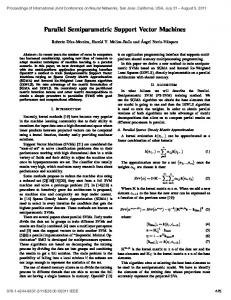
Figure 1. Best viewed in colour. Locally linear svm classifier for banana function data set. Red and green points correspond to positive and negative samples, black stars correspond to the anchor points and blue lines are obtained decision boundary. Even though the problem is obviously not linearly separable, locally in sufficiently small regions the decision boundary is nearly linear and thus the data can be separated reasonably well using local linear classifier.
where HW,b (xk ) = (γ(xk )T Wxk + γ(xk )T b), S is the set of training samples, xk the feature vector and yk ∈ {−1, 1} is the correct label of the k-th sample. We will call the classifier obtained by this optimisation procedure locally linear svm (ll-svm). This formulation is very similar to standard linear svm formulation over nm dimensions except there are several biases. This optimisation problem can be converted to a qp problem with quadratic cost function subject to linear constraints similarly to standard svm as: 1 X λ ξk ||W||2 + arg minW,b (10) 2 |S| k∈S
s.t.∀k ∈ S :
ξk ≥ 0 ξk ≥ 1 − yk (γ(xk )T Wxk + γ(xk )T b).
Solving this qp problem can be rather expensive for large data sets. Even though decomposition methods such as smo (Platt, 1998; Chang & Lin, 2001) or svmlight (Joachims, 1999) can be applied to the dual representation of the problem, it has been experimentally shown that for real applications they are outperformed by stochastic gradient descent methods. We adapt the SVMSGD2 method proposed in (Bordes et al., 2009) to tackle the problem. Each iteration of SVMSGD2 consists of picking random sample xt and corresponding label yt and updating the current solution of the W and b if the hinge loss cost 1 − yt (γ(xt )T Wxt + γ(xt )T b) is positive as: Wt+1
=
bt+1
=
1 yt (xt γ(xt )T ) λ(t + t0 ) 1 bt + yt γ(xt ), λ(t + t0 ) Wt +
where Wt and bt is the solution after t iterations, 1 xt γ(xt )T is the outer product and λ(t+t is the opti0) mal learning rate (Shalev-Shwartz et al., 2007) with a heuristically chosen positive constant t0 (Bordes et al., 2009), that ensures the first iterations do not produce too large steps. Because local codings either force (Roweis & Saul, 2000; Wang et al., 2010) or induce (Gao et al., 2010; Yu et al., 2009) sparsity, the update step is done only for a few columns with nonzero coefficients of γ(x). Regularisation update is done every skip iterations to speed up the process similarly to (Bordes et al., 2009) as: skip 0 Wt+1 = Wt+1 (1 − ). (13) t + t0 Because the proposed model is equivalent to a sparse mapping into the higher dimensional space, it has the same theoretical guarantees as standard linear svm and for given number of anchor points m is slower than linear svm only by a constant factor independent on the size of the training set. In case the stochastic gradient method does not converge in one pass and local coordinates were expensive to evaluate, they can be evaluated once and kept in the memory. This binary classifier can be extended to multi-class one either by following standard one vs. all strategy or using the formulation of (Crammer & Singer, 2002).
(11)
3.1. Relation and comparison to other models
(12)
Conceptually similar local linear classifier has been already proposed by (Zhang et al., 2006). Their knn-
Locally Linear Support Vector Machines
Algorithm 1 stochastic gradient descent for ll-svm. Input: λ, t0 , W0 , b0 , T , skip, C Output: W, b t = 0, count = skip, W = W0 , b = b0 while t ≤ T do γt = LocalCoding(xt , C) Ht = 1 − yt (γtT Wxt + γtT b) if Ht > 0 then 1 W = W + λ(t+t yt (xt γtT ) 0) 1 b = b + λ(t+t0 ) yt γt end if count = count − 1 if count ≤ 0 then skip ) W = W(1 − t+t 0 count = skip end if t=t+1 end while svm linear svm classifier was optimized for each test sample separately as a linear svm using k nearest neighbours of the given test sample. Unlike our model, their classifier has no closed form solution resulting in the significantly slower evaluation, and requires keeping all the training samples in memory in order to quickly find nearest neighbours, which may not be suitable for too large data sets. Our classifier can be also seen as a bilinear svm where one input vector depends nonlinearly on another one. A different form of bilinear svm has been proposed in (Farhadi et al., 2009) where one of the input vectors is randomly initialized and iteratively trained as a latent variable vector alternating with the optimisation of weight matrix W. llsvm classifier can be also seen as a finite kernel svm. The transformation function associated with the kernel transforms the classification problem from n to nm dimensions and any optimisation method can be applied in this new feature space. Another interpretation of the model is that the classifier is the weighted sum of linear svms for each anchor point where the individual linear svms are tied together during the training process with one hinge loss cost function. Our classifier is more general than standard linear svm. Any linear svm over the original P feature values can be expressed due to the property v∈C γv (x) = 1 by a matrix W with each row equal to w of the linear classifier and bias b vector with each value equal to the bias of the linear classifier as: H(x) = = =
γ(x)T Wx + γ(x)T b (14) T T T T γ(x) (w , w , ..)x + γ(x) (b, b, ..) wT x + b.
ll-svm classifier is also more general than the linear svm over local coordinates γ(x) as applied in (Yu et al., 2009), because the vector of weights of any linear svm classifier over these variables can be represented using W = 0 as a linear combination of the set of biases: H(x) = γ(x)T Wx + γ(x)T b = bT γ(x).
(15)
3.2. Extension to finite dimensional kernels In many practical cases learning the highly non-linear decision boundary of the classifier would require a high number of anchor points. This could lead to overfitting of the data or significant slow-down of the method. To overcome this problem we can trade-off the number of anchor points against the expressivity of the classifier. Several practically useful kernels, for example intersection kernel used for bag-of-words models (Vedaldi et al., 2009), can be approximated by finite kernels (Maji & Berg, 2009; Vedaldi & Zisserman, 2010) and resulting svm optimised using stochastic gradient descent methods (Bordes et al., 2009; Shalev-Shwartz et al., 2007). Motivated by this fact, we extend the local classifier to the svms with any finite dimensional kernel. Let the kernel operation be de˙ 2 ). fined as or approximated by K(x1 , x2 ) = Φ(x1 )Φ(x Then the classifier will take the form: H(x) = γ(x)T WΦ(x) + γ(x)T b.
(16)
where parameters W and b are obtained by solving: arg minW,b
λ 1 X ξk ||W||2 + 2 |S|
(17)
k∈S
s.t.∀k ∈ S :
ξk ≥ 0 ξk ≥ 1 − yk (γ(xk )T WΦ(xk ) + γ(xk )T b)
and the same stochastic gradient descent method to the one in the section 3 could be applied. Local coordinates can be calculated in either the original space or the feature space, this depends on where we assume more meaningful manifold structure.
4. Experiments We tested ll-svm algorithm on three multi label classification data sets of digits and letters - mnist, usps and letter. We compared the performance to several binary and multi label classifiers in terms of accuracy and speed. Classifiers were applied directly to the raw data without calculating any complex features in order to get a fair comparison of classifiers. Multi-class experiments were done using standard one vs. all strategy.
Locally Linear Support Vector Machines
mnist data set contains 40000 training and 10000 test gray-scale images of the resolution 28 x 28 normalized into 784 dimensional vector. Every training sample has a label corresponding to one of the 10 digits 0 00 −0 90 . The manifold was trained using k-means clustering with 100 anchor points. Coefficients of the local coding were obtained using inverse Euclidian distance based weighting (Gemert et al., 2008) solved for 8 nearest neighbours. The reconstruction error minimising codings (Roweis & Saul, 2000; Yu et al., 2009) did not lead to a boost of performance. The evaluation time given local coding is O(kn), where k is the number of nearest neighbours. The calculation of k nearest neighbours given their distances from anchor points takes O(km) which is significantly faster. Thus, the bottle-neck is the calculation of distances from anchor points which runs in O(mn) with approximately the same constant as the svm evaluation. To speed it up, we calculated the distance of every 2 × 2 dimension and if it was already higher than the final distance of the k-th nearest neighbour, we rejected the anchor point. This led to an 2× speedup. A comparison of performance and speed to the state-of-the-art methods is given in table 1. The dependency of performance on the number of anchor points is depicted in figure 2. The comparisons to other methods show, that ll-svm can be seen as a good trade-off between qualitatively best kernel methods and very fast linear svms. usps data set consists of 7291 training and 2007 test gray-scale images of the resolution 16 x 16 stored as 256 dimensional vector. Each label corresponds to the one of the 10 digits 0 00 −0 90 . The letter data set consists of 16000 training and 4000 testing images represented as a relatively short 16 dimensional vector. The labels correspond to the one of the 26 letters 0 A0 −0 Z 0 . Manifolds for these data sets were learnt using the same parameters as for mnist data set. Comparisons to the state-of-the-art methods in these two data sets in terms of accuracy and speed is given in table 2. The comparisons on these smaller data sets show that ll-svm requires more data to compete with the stateof-the-art methods. The algorithm has also been tested on the Caltech101 data set (Fei-Fei et al., 2004), that contains 102 object classes. The multi label classifier was trained using 15 training samples per class. The performance of both ll-svm and locally additive kernel svm with the approximation of the intersection kernel has been evaluated. Both classifiers were applied to the histograms of grey and colour PHOW (Bosch et al., 2007) descriptors (both 600 clusters), and self-
Figure 2. Dependency of the performance of ll-svm on number of anchor points on mnist data set. Standard linear svm is equivalent to the ll-svm with one anchor point. The performance is saturated at around 100 anchor points due to insufficiently large amount of training data.
similarity (Shechtman & Irani, 2007) feature (300 clusters) on the spatial pyramid (Lazebnik et al., 2006) 1 × 1, 2 × 2 and 4 × 4. The final classifier was obtained by averaging the classifiers for all histograms. Only the histograms over the whole image were used to learn the manifold and obtain the local coordinates, resulting in the significant speed-up. The manifold was learnt using k-means clustering with only 20 clusters due to insufficient amount of training data. Local coordinates were computed using inverse Euclidian distance weighting on 5 nearest neighbours.
5. Conclusion In this paper we propose a novel locally linear svm classifier using nonlinear manifold learning techniques. Using the concept of local linearity of functions defining decision boundary and properties of manifold learning methods using local codings, we formulate the problem and show how this classifier can be learned either by solving the corresponding qp program or in an online fashion by performing stochastic gradient descent with the same convergence guarantees as standard gradient descent method for linear svm. Experiments show that this method gets close to state-ofthe-art results for challenging classification problems whilst being significantly faster than any competing algorithms. The complexity grows linearly with the size of the data set and thus the algorithm can be applied to much larger data sets. This may become a major issue as many new large scale image and natural language processing data sets gathered from internet are emerging.
Reference Balcan, M.-F., Blum, A., and Vempala, S. Kernels as features: On kernels, margins, and low-dimensional mappings. In ALT, 2004. Boiman, O., Shechtman, E., and Irani, M. In defense of
Locally Linear Support Vector Machines
Table 1. A comparison of the performance, training and test times of ll-svm with the state-of the art algorithms on mnist data set. All kernel svm methods (Chang & Lin, 2001; Bordes et al., 2005; Crammer & Singer, 2002; Tsochantaridis et al., 2005; Bordes et al., 2007) used rbf kernel. Our method achieved comparable performance to the state-of-the-art and could be seen as a good trade-off between very fast linear svm and the qualitatively best kernel methods. ll-svm was approximately 50-3000 times faster than different kernel based methods. As the complexity of kernel methods grow more than linearly, we expected larger relative difference for larger data sets. Running times of mcsvm, svmstruct and la-rank are as reported in (Bordes et al., 2007) and thus only illustrative. N/A means the running times are not available.)
Method Linear svm (Bordes et al., 2009) (10 passes) Linear svm on lcc (Yu et al., 2009) (512 a.p.) Linear svm on lcc (Yu et al., 2009) (4096 a.p.) Libsvm (Chang & Lin, 2001) la-svm (Bordes et al., 2005) (1 pass) la-svm (Bordes et al., 2005) (2 passes) mcsvm (Crammer & Singer, 2002) svmstruct (Tsochantaridis et al., 2005) la-rank (Bordes et al., 2007) (1 pass) ll-svm (100 a.p., 10 passes)
error 12.00% 2.64% 1.90% 1.36% 1.42% 1.36% 1.44% 1.40% 1.41% 1.85%
training time 1.5 s N/A N/A 17500 s 4900 s 12200 s 25000 s 265000 s 30000 s 81.7 s
test time 8.75 µs N/A N/A 46 ms 40.6 ms 42.8 ms N/A N/A N/A 470 µs
Table 2. A comparison of error rates and training times for ll-svm and the state-of the art algorithms on usps and letter data sets. ll-svm was significantly faster than kernel based methods, but it requires more data to achieve results close to the state-of-the-art. The training times of competing methods are as they were reported in (Bordes et al., 2007). Thus they are not directly comparable, but give a broad idea about the time consumptions of different methods.
Method Linear svm (Bordes et al., 2009) mcsvm (Crammer & Singer, 2002) svmstruct (Tsochantaridis et al., 2005) la-rank (Bordes et al., 2007) (1 pass) ll-svm (10 passes)
error 9.57% 4.24% 4.38% 4.25% 5.78%
usps training time 0.26 s 60 s 6300 s 85 s 6.2 s
error 41.77% 2.42% 2.40% 2.80% 5.32%
letter training time 0.18 s 1200 s 24000 s 940 s 4.2 s
Table 3. A comparison of the performance, training and test times for the locally linear, locally additive svm and the state-of the art algorithms on caltech (Fei-Fei et al., 2004) data set. Locally linear svm obtained similar result as the approximation of the intersection kernel svm designed for bag-of-words models. Locally additive svm achieved competitive performance to the state-of-the-art methods. N/A means the running times are not available.
Method Linear svm (Bordes et al., 2009) (30 passes) Intersection kernel svm (Vedaldi & Zisserman, 2010) (30 passes) svm-knn (Zhang et al., 2006) llc (Wang et al., 2010) mkl (Vedaldi et al., 2009) nn (Boiman et al., 2008) Locally linear svm (30 passes) Locally additive svm (30 passes)
accuracy 63.2% 68.8% 59.1% 65.4% 71.1% 72.8% 66.9% 70.1%
training time 605 s 3680 s 0s N/A 150000 s N/A 3400 s 18200 s
test time 3.1 ms 33 ms N/A N/A 1300 ms N/A 25 ms 190 ms
Locally Linear Support Vector Machines
nearest-neighbor based image classification. CVPR, 2008. Bordes, A., Ertekin, S., Weston, J., and Bottou, L. Fast kernel classifiers with online and active learning. JMLR, 2005. Bordes, A., Bottou, L., Gallinari, P., and Weston, J. Solving multiclass support vector machines with larank. In ICML, 2007. Bordes, A., Bottou, L., and Gallinari, P. Sgd-qn: Careful quasi-newton stochastic gradient descent. JMLR, 2009. Bosch, A., Zisserman, A., and Munoz, X. Representing shape with a spatial pyramid kernel. In CIVR, 2007. Breiman, L. Random forests. In Machine Learning, 2001. Chang, C. and Lin, C. Libsvm: A Library for Support Vector Machines, 2001. Cortes, C. and Vapnik, V. Support-vector networks. In Machine Learning, 1995. Crammer, K. and Singer, Y. On the algorithmic implementation of multiclass kernel-based vector machines. JMLR, 2002. Dalal, N. and Triggs, B. Histograms of oriented gradients for human detection. In CVPR, 2005. Farhadi, A., Tabrizi, M.K., Endres, I., and Forsyth, D.A. A latent model of discriminative aspect. In ICCV, 2009. Fei-Fei, L., Fergus, R., and Perona, P. Learning generative visual models from few training examples an incremental bayesian approach tested on 101 object categories. In Workshop on GMBS, 2004. Freund, Y. and Schapire, R. E. A short introduction to boosting, 1999. Gammerman, A., Vovk, V., and Vapnik, V. Learning by transduction. In UAI, 1998. Gao, S., Tsang, I. W.-H., Chia, L.-T., and Zhao, P. Local features are not lonely - laplacian sparse coding for image classification. In CVPR, 2010.
Joachims, Thorsten. Making large-scale support vector machine learning practical, pp. 169–184. MIT Press, 1999. Lazebnik, S., Schmid, C., and Ponce, J. Beyond bags of features: Spatial pyramid matching for recognizing natural scene categories. In CVPR, 2006. Maji, S. and Berg, A. C. Max-margin additive classifiers for detection. ICCV, 2009. Platt, J. Fast training of support vector machines using sequential minimal optimization. In Advances in Kernel Methods - Support Vector Learning. MIT Press, 1998. Roweis, S. T. and Saul, L. K. Nonlinear dimensionality reduction by locally linear embedding. Science, 290: 2323–2326, 2000. Shakhnarovich, G., Darrell, T., and Indyk, P. Nearestneighbor methods in learning and vision: Theory and practice, 2006. Shalev-Shwartz, S., Singer, Y., and Srebro, N. Pegasos: Primal estimated sub-gradient solver for svm. In ICML, 2007. Shechtman, E. and Irani, M. Matching local selfsimilarities across images and videos. In CVPR, 2007. Tsochantaridis, I., Joachims, T., Hofmann, T., and Altun, Y. Large margin methods for structured and interdependent output variables. JMLR, 2005. Vapnik, V. and Lerner, A. Pattern recognition using generalized portrait method. automation and remote control, 1963. Vedaldi, A. and Zisserman, A. Efficient additive kernels via explicit feature maps. In CVPR, 2010. Vedaldi, A., Gulshan, V., Varma, M., and Zisserman, A. Multiple kernels for object detection. In ICCV, 2009. Wang, J., Yang, J., Yu, K., Lv, F., Huang, T. S., and Gong, Y. Locality-constrained linear coding for image classification. In CVPR, 2010. Yu, K., Zhang, T., and Gong, Y. Nonlinear learning using local coordinate coding. In NIPS, 2009.
Gemert, J. C. Van, Geusebroek, J., Veenman, C. J., and Smeulders, A. W. M. Kernel codebooks for scene categorization. In ECCV, 2008.
Zhang, H., Berg, A. C., Maire, M., and Malik, J. Svmknn: Discriminative nearest neighbor classification for visual category recognition. CVPR, 2006.
Guyon, I., Boser, B., and Vapnik, V. Automatic capacity tuning of very large vc-dimension classifiers. In NIPS, 1993.
Zhou, X., Cui, N., Li, Z., Liang, F., and Huang, T.S. Hierarchical gaussianization for image classification. In ICCV, 2009.