PRAMANA — journal of
c Indian Academy of Sciences °
physics
Vol. 75, No. 3 September 2010 pp. 549–563
Locating phase transitions in computationally hard problems B ASHOK1,∗ and T K PATRA2,3 1
Advanced Centre of Research in High Energy Materials, University of Hyderabad, Central University P.O., Gachi Bowli, Hyderabad 500 046, India 2 School of Physics, University of Hyderabad, Central University P.O., Gachi Bowli, Hyderabad 500 046, India 3 Present address: Department of Chemical Engineering, Indian Institute of Technology, Kanpur 208 016, India ∗ Corresponding author. E-mail:
[email protected];
[email protected] MS received 4 March 2010; revised 9 April 2010; accepted 13 April 2010 Abstract. We discuss how phase-transitions may be detected in computationally hard problems in the context of anytime algorithms. Treating the computational time, value and utility functions involved in the search results in analogy with quantities in statistical physics, we indicate how the onset of a computationally hard regime can be detected and the transit to higher quality solutions be quantified by an appropriate response function. The existence of a dynamical critical exponent is shown, enabling one to predict the onset of critical slowing down, rather than finding it after the event, in the specific case of a travelling salesman problem (TSP). This can be used as a means of improving efficiency and speed in searches, and avoiding needless computations. Keywords. New applications of statistical mechanics; analysis of algorithms; heuristics; phase transitions and critical phenomena. PACS Nos 89.75.-k; 05.70.Fh; 64.60.Bd; 64.60.A-
1. Introduction Everyday computational situations are replete with cases where the solution quality does not seem to justify the time spent in generating the answer, while a quick even if less accurate solution would have been as satisfactory. In the following sections, we describe how detection of phase transitions in computational problems may be done, within a framework of statistical mechanics of thereby avoiding regimes wherein computational efforts put in are not commensurate with the solution obtained. This would be of utmost importance especially in situations where the problem being solved is an NP (nondeterministic polynomial time) hard problem, or where there is a transition in the very nature of the problem from an easily computable regime to one that is very hard to solve. To be able to actually predict 549
B Ashok and T K Patra a phase transition in a computational context (not just find it subsequently) and to predict and avoid the ‘critical slowing down regime’ has not, to the best of our knowledge, been demonstrated before. We discuss this in detail in the context of anytime algorithms. This framework has been completely explained in this paper itself, so that this work is self-contained and complete. We have implemented this method here, yielding very interesting and significant results. There is a considerable body of literature dealing with the travelling salesman problem and with phase transitions and their use in constraint satisfaction problems [1,11]. While the use of phase transitions in search problems in general has been extensively investigated, there does not seem to have been an attempt to try to use phase transitions in anytime algorithms as a means of monitoring the progress of the algorithm or in any other form. We show that a critical exponent can be found that relates the time taken to come to a stable solution quality preceding a phase transition, to the number of nodes or cities of a travelling salesman problem. This is a new and important result that has not been reported in the literature, as far as we know. The existence of a critical exponent makes it possible to predict when the onset of a computationally hard regime would take place. This is of great importance as it has long been unclear how to efficiently run algorithms especially when one has to make a trade-off between solution quality and the computational time needed to achieve an acceptable, near-optimal solution, given the constraints of time. The particular problem used – the travelling salesman problem – is only illustrative of the theoretical approach we suggest for detecting phase transitions. We show how this relatively simple approach may be used in any other search and optimization problem so that computational time may be vastly reduced by halting the running of an algorithm when a near-optimal solution is reached prior to a phase transition to a computationally hard regime. It would be of interest to see if phase transitions could be used in conjunction with anytime algorithms as a means of further improving the accuracy and speed in searches. 2. A brief sketch of anytime algorithms Anytime algorithms are algorithms whose execution can be stopped at any time, giving a solution to the problem being solved. The quality of the solution improves with time [12,13]. These algorithms become specially important when we are faced with constraints, which might include, among other things, the computational resources and the time available to us to solve the problem. Thus, to satisfy the constraints put on it, an anytime algorithm trades-off between the solution quality and the computational time, for example. The two main types of anytime algorithms are contract and interruptible algorithms. Contract algorithms run for a fixed length of time, and give a solution only when that interval of time elapses. Interruptible algorithms form a larger family – they may be interrupted at any stage to obtain an answer though the accuracy and the meaningfulness of the solution would, of course, vary. Monitoring an anytime algorithm is very important as we can keep track of the progress of the algorithm and decide when and at what intervals we could monitor or stop the algorithm in order to obtain an optimal answer optimally.
550
Pramana – J. Phys., Vol. 75, No. 3, September 2010
Locating phase transitions in computationally hard problems Some quantities play a very basic part in such algorithms. A performance profile gives us a measure of the expected quality of the output with the execution time. A performance profile is thus typically a probability distribution. Those performance profiles we have tacitly used are actually dynamic performance profiles, P r(Qj |Qi , ∆t), which is the probability of obtaining a solution of quality Qj by resuming the algorithm for a time interval ∆t when the current solution has quality Qi . A utility function U (Qi , tk ) tells us the utility of a solution of quality Qi at time tk [13]. Hansen and Zilberstein [13] had chosen a monitoring policy m for tracking the progress of an algorithm such that it maximizes a value function V (fr , tk ), a cost function C1 being introduced to include the cost of monitoring. As one can only estimate the true solution quality at any given time, a feature fr is made the basis for estimating the solution quality Qi . Use is made of partial observability functions like P r(Qi |fr , tk ) and P r(fr |Qi , tk ) in the value function above to estimate improvements in quality. The algorithm is accordingly monitored or allowed to run or halted, as dictated by the monitoring policy. Our approach is somewhat different, as explained in the next section. 3. Phase transitions and anytime algorithms Although phase transitions occur only in the thermodynamic limit, in the limit of infinitely large systems, as was first pointed out by Kramers [14], finite state transitions nevertheless exhibit similarities to true phase transitions and hence are very much relevant to computational situations. Singularities and singular behaviour could be used to define universality classes on the basis of common characteristics like, for example, swiftly changing correlation lengths between parts of a system at and near the point of transition. Phase transitions have appeared in a number of computational contexts and paradigms (see, for example [5,8,11], and references therein). The transition from a polynomial to exponential search costs, the transition from an underconstrained to overconstrained problem, the appearance of transitions in optimization problems, automatic planning and models of associative memory among others, all indicate the widespread prevalence of phase transitions in a computational context. It has also been found that, on an average, several search heuristics have hard problem instances concentrated at similar parametric values which points correspond to transitions in solubility. When one wishes to employ an anytime algorithm for getting a quick, approximate solution to a problem, the question that arises is how long is long enough before stopping the execution of the algorithm and deciding to accept a solution? Can one decide beforehand, on a systematic basis, the length of this run-time? For a problem, the time of onset of a transition to a computationally hard regime wherein the solution quality does not significantly improve enough to justify running the algorithm for a longer time, could act as one criterion for deciding the run-time. Detecting such a transition requires one to run the algorithm unmindful of solution quality so that any change in behaviour that quantifies the transition can be located. This is what we have done in this paper. Another requirement is to describe the particular computational problem being considered using some more quantifiable terms. Several authors have addressed
Pramana – J. Phys., Vol. 75, No. 3, September 2010
551
B Ashok and T K Patra combinatorial problems through ideas from statistical mechanics; a good review of the literature can be found in [11] and references therein. Gent and Walsh [15] addressed, in particular, the problem of a phase transition for the travelling salesman problem. They identified a transition between soluble and insoluble instances of the decision problem (namely, whether or not a tour of some length l or less exists for the given TSP), at some critical value of a parameter. In physical systems, a transition from liquid to gaseous states, or from paramagnetic to ferromagnetic states for magnetic systems, can be well described using the behaviour of the thermodynamical potentials and response functions like susceptibility and order parameters like the magnetization (see for example ref. [16]). In the following sections, we present a formalism for quantifying phase transitions in the computational context. The test-problem that we study in this paper is that of obtaining a near-optimal solution for a two-dimensional TSP with N nodes or cities distributed randomly over a unit square. The premise is that any change in behaviour of the computational time of the algorithm would be detected, enabling us to quantify any transition to a computationally hard regime. The challenge that we face here is how to draw an analogy between thermodynamic potentials and response functions for a physical system to quantities in a more abstract system such as a computational problem and algorithm. 4. Defining the formalism in analogy with statistical physics In this paper, we consider the two-dimensional TSP as the toy problem to test our formalism. In keeping with expectations that any phase transition in a system should be distinctly observable, we first decide to look for a drastic transition in various quantities like the quality of a solution and the value function. The actual utility of a solution at any instant depends upon its quality, as well as the rate of improvement shown by the quality and the computational time needed to arrive at it. The utility can be expected to increase in direct proportion to both the quality of the solution as well as the rate of improvement of quality, whereas it reduces in direct proportion to the increasing computational time required. We therefore make an ansatz that a utility function denoted by U (Qi , Q˙ i , tk ) can be defined with these properties, and which in the simplest instance has a linear dependence on Q ˙ and Q: U (Qi , Q˙ i , tk ) = a1 Qi + a2 Q˙ i − a3 t. (1) We have taken a1 , a2 and a3 to be positive constants. The quality function Qi can be defined in several ways, depending upon the particular problem being considered. For the TSP, one obvious choice for Qi would be the reduction in path-length over each iteration, because one wishes to complete a tour as optimally as possible. We hence choose to define quality by Qi ≡
(Li − Lc ) , Li
(2)
where Li is the initial path length and Lc is the current path length. The value function (mentioned in §2) used is taken as a sum of the expected values of the utility function, and is defined by 552
Pramana – J. Phys., Vol. 75, No. 3, September 2010
Locating phase transitions in computationally hard problems V (fk , tk ) =
X
P r(Qj |fk , tk , ∆t)U (Qj , Q˙ j , tk + ∆t).
(3)
j
In the toy model being discussed, we will take the feature fk to be the quality Qk , so that V (Qk , tk ) defines in quantitative terms the value of a solution of quality Qk at time tk in obtaining other solutions of quality Qj in a time step following tk . The utility U (Qj , Q˙ j , tk + ∆t) when weighted by the conditional probability of obtaining that solution of quality Qj in time step ∆t after starting at time tk with quality Qk , and summed over all Qj , clearly gives a measure of the value of the solution of quality Qk . Hence the definition (3) of the value function. The procedure adopted is as follows. 2-opt heuristics is employed to solve each problem instance. To calculate and generate a performance profile, the algorithm is run for about 500 times. To then solve a particular problem, the performance profile generated earlier is used on completion of each iteration of the algorithm to calculate quantities like the value function. The initial tour is generated by means of a nearest-neighbour algorithm. The steps of the initial tour construction are: 1. 2. 3. 4.
Select a random city. Find the nearest unvisited city and go there. If any unvisited cities are left, repeat the previous step. Return to the first city.
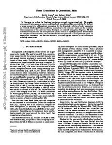
Tour improvement is done through a 2-opt heuristic, i.e., following initial tour construction, in subsequent iterations, the algorithm selects a small segment of the sequence and reverses it. We use a simple 2-bond move which reverses the sequence of cities for a chosen segment to obtain a trial tour. In each iteration of this 2opt heuristic, we accept a tour if it is shorter than the previous one, rejecting it otherwise. Solution quality therefore keeps improving or remains unchanged, as long as time permits. On completion of each iteration of our algorithm, we use the performance profile generated earlier to calculate the value function and the cost inflection function described below. Data from 500 samples are averaged for obtaining each point in the data sets used to draw our inferences. The frequency with which a certain quality Q is achieved is shown in figure 1 for a travelling salesman tour with the number of nodes N = 30, 50 and 70. The quality is found to obey a distribution of the form P (Q) = α exp(βQ − γQ3 ),
(4)
where α, β and γ are N -dependent, positive parameters. The question thus arises – how do we locate or predict a phase transition in a problem such that it can be of practical importance and used? To deal with this, we define a function K, which we call the cost inflection function, the suddenly changing behaviour of which would indicate the occurrence of a phase transition. Since we want a good solution as soon as possible, with minimal time elapse, we could think of K as the value of the solution corrected to account for the time expended in arriving at it. We make the ansatz that the cost inflection function K(Qi , ti ) is related to the value function V (Qi , t) and to solution quality through the relation K(Qi , t) = V (Qi , t) − tQi ,
(5)
Pramana – J. Phys., Vol. 75, No. 3, September 2010
553
B Ashok and T K Patra
Figure 1. Frequency of occurrence of different quality values for an algorithm for a TSP for N = 30, 50 and 70, over 106 instances. The distribution obeyed is eq. (4), with α, β and γ values being approximately given as 72.57, 43.67, 255.45, respectively for N = 30; 242.72, 46.31, 425.31, respectively for N = 50 and 317.69, 51.55, 617.56, respectively for N = 70. 0 -50
V
-100
N = 100 N = 250 N = 300 N = 350
-150 -200 -250 -300
1
10
t
100
1000
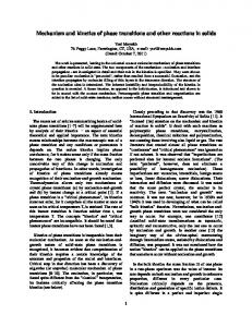
Figure 2. Plot of the value function V as a function of time t, for different cases of TSP with number of nodes N = 100, 250, 300 and 350.
where the value V (Qi , t) is defined by eq. (3), Qi being the quality function of the currently available solution. Figures 2 and 3 show the dependence between cost inflection, value and quality functions. As can be clearly seen, the cost inflection function shows a marked change in behaviour after a particular point. We identify K as an analogue to the Helmholtz free energy A. Recall that the value function is a weighted sum of the utility function. The value function’s temporal evolution (figure 2) reminds us of the time evolution of the most probable value Xm of the number of particles (corresponding to the chemical composition) for a system in the stochastic theory of adiabatic explosion [17]. In that thermodynamic system, Xm evolves with time till some critical time tc after which new solution branches appear corresponding to other probability states. In a system undergoing combustion, this is the temporary situation where the molecules can be differentiated into a part for which combustion has not yet taken place and a part for which combustion has ended. In our problem, the evolution of V (fi , t) 554
Pramana – J. Phys., Vol. 75, No. 3, September 2010
Locating phase transitions in computationally hard problems N=350 N=250 N=150
V
50 0 -50 -100 -150 -200 -250 -300
0 0.02 0.04 0.06 0.08 Q
-50
0.1 -150 -100 0.12 -250 -200 0.14-350 -300 K
0
50
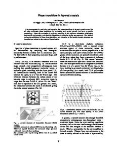
Figure 3. Three-dimensional plot of cost inflection, quality and value functions, for N = 150, 250 and 350.
N=250 ..
0.12
V
0.1 0.08
25 20 15 10 5 0 -5 -10 -15 -20 -25
0.06 0.04 0.02 0 0 -10 -20 -30 -40 -50 -60 -70 -80 -90 50 75 -100
K
1 5
t
10 25
Figure 4. The second derivative of the value function with respect to time, V¨ , plotted as a function of K and time t, the quality of the solution, Q, being depicted by the colour; number of nodes N = 250. Note the sharp inflection corresponding to a phase transition.
is an evolution of the system to higher quality solutions, differentiated by a point of inflection at a time t = tc where the system slows down heralding the onset of critical slowing down. The appearance of a symmetric spike in the V¨ profile plotted as a function of t and K, and a sharp inflection of the curve into another plane, as shown in figure 4, are symptomatic of a major transition in quality, and is accompanied by a transition to a different computational regime. In figure 5 we have plotted the improvement of solution quality with time for the TSP defined above, for different values of N . We find that the behaviour of Q can
Pramana – J. Phys., Vol. 75, No. 3, September 2010
555
B Ashok and T K Patra
0.1
Q
N = 100 N = 200 N = 250 0.1253*exp(-7.66/t)
0.05
0
20
40
80
60
t
100
Figure 5. The quality function plotted as a function of time for three values of N (N = 100, 200, 250), and an overlaying plot of an Arrhenius function, to show the broad qualitative similarity. N=100
N=30 0.08 0.07 0.06 0.05 0.04 0.03 0.02 0.01 0
..
K 20 15 10 5 0 -5 -10 -15 -20
7 6 5
0.09 0.08 0.07 0.06 0.05 0.04 0.03 0.02 0.01 0
..
K 100 80 60 40 20 0 -20 -40 -60 -80 -100
15 10 5
4 3
0.01
K
2
0.1 1
t
0.1
1
1
10 0
10
t
0 -5 -10 -15 100-20
K
N=200 N=300 ..
K
.. 0.12 0.1 0.08 0.06 0.04 0.02 0
K 20 15 10 5 0 -5 -10 -15 -20
0
0.1 1
t
10
-10 -20 -30 -40 -50 -60 K -70 -80 -90 -100
0.09 0.08
500 400 300 200 100 0 -100 -200 -300 -400 -500
0.07 0.06 0.05 0.04 0.03 0.02 0.01
1 10
t
100
0 -50 -100 -150 -200 K -250 -300 -350 1000
50
¨ −Q plots obtained for TSP with N = 30, Figure 6. Representative K −t− K ¨ corresponds 100, 200 and 300. K is the cost inflection function, t the time, K to the second derivative of K with respect to time. Q, the quality function, is represented by the colour.
556
Pramana – J. Phys., Vol. 75, No. 3, September 2010
Locating phase transitions in computationally hard problems
Figure 7. Efficacy CN plotted as a function of time t (a) for different number of nodes N , all showing a transition to a stable regime where CN stable ∝ t2 ; (b) for N = 175 at left, and N = 300 at right: representative plots showing the regime of CN = CN stable to correspond to the high quality metastable and stable states.
be approximated by means of an Arrhenius equation Qapprox = b exp(−c/t),
(6)
where b and c are some real constants. The suffix approx has been added to Q to stress that this is but a tool in our gedankenexperiment to help understand a rather abstract system in terms more familiar to us. This form of Qapprox is almost exactly like the Arrhenius law for the rate constant w(T ) in a chemical reaction in a combustive process w(T ) = A exp(−E/RT ), E being the activation energy, R the gas constant, T the temperature and A the pre-exponential or frequency factor that can be approximated to be constant. Just as in the thermodynamic situation, Pramana – J. Phys., Vol. 75, No. 3, September 2010
557
B Ashok and T K Patra
100
tc
10
1
10
N
100
Figure 8. Plot indicating dependence of tc , time of onset of critical slowing down, on number of nodes N . The best fit for the log–log plot is the equation tc = a0 N z , where a0 = 0.00047 ± 0.00027, z = 2.073 ± 0.099. 0.9
Lo = 0.7408 N
1/2
+ 1.1732
0.86
Lo/N
1/2
0.88
0.84 0.82 0.8 0.05
0.075
0.1
0.125
0.15
1/2
1/N
√ √ Figure 9. Plot of Lo / N vs.√1/ N , Lo being optimal length. The plot obeys eq. (22), Lo (N ) = 0.7408 N + 1.1732.
the rate constant increases rather steeply with temperature, eventually plateauing out to a constant value, in our case the solution quality too increases quickly with time before approaching the maximum achievable value for the problem. As in thermodynamics, in our computational context too one can define appropriate response functions. As time elapses, the system responds by a perceptible change in its quality. This is reflected as a decrease in the cost inflection function K after a critical value (see figure 6). This motivates us to define a quantity CN , for which we coin the term efficacy of the algorithm: ¨ CN = |tK|,
(7)
where derivatives are with respect to time. The cost inflection function K is calculated from eq. (5). A plot of the efficacy function, CN , as a function of time t for different N values (figures 7a and b) shows an interesting observation – CN tends to show almost random behaviour upto a point where a transition to a stable regime takes place; thereafter, the efficacy function shows a strict t dependence 558
Pramana – J. Phys., Vol. 75, No. 3, September 2010
Locating phase transitions in computationally hard problems CN stable ∝ t.
(8)
This stable area, as can be seen in figure 7b, corresponds to regimes where the quality Q has reached its maximal value, or is reaching it, and encompasses, therefore, both stable and metastable states. The efficacy as defined above therefore makes a very good response function in identifying a transition to a near-optimal set of regimes. In the thermodynamic context, the specific heat Cv for a fluid is, as we know, defined by µ 2 ¶ ∂A Cv = −T , (9) ∂T 2 v where A denotes the Helmholtz free energy. The specific heat behaviour as a function of temperature is distinct, depending upon whether the temperature is below or above a critical temperature Tc for the thermodynamic system. For example, for the well-known superfluid or λ transition in 4 He the specific heat dependence can be approximated by C ≈ A log(T − Tλ ) + B, for temperatures above the critical λ-transition temperature T > Tλ , and C ≈ A0 log(Tλ − T ) + B 0 for temperatures below the critical temperature T < Tλ , with the prefactors A, B, A0 and B 0 being temperature-independent constants [18]. In our case, the response function CN is such that its behaviour changes abruptly at the point corresponding to a critical value of elapsed time for the system. In other words, looking at CN , we should clearly be able to distinguish between separate phases or regimes. Approach to a phase transition or bifurcation point in physical systems is typically characterized by a critical slowing down. We therefore expect that our system should show similar behaviour. In the TSP under consideration, critical slowing down would correspond to a regime wherein solution quality remains unchanged over a comparatively long period of time, whereas other measures of algorithm efficiency, like the cost inflection function K, or the value function V , tend to show a change in behaviour. An investigation of our data indicates that the onset of critical slowing down in the algorithm can be quantified and detected. Locating tc , the time of onset of this critical slowing down, is quite straightforward. It should be noted that there may be more than one regime where the solution quality of the algorithm lingers at one value for an extended period of time. Such states may essentially be thought of as metastable states for the system, as has been mentioned in our discussion of the efficacy function. However, tc is distinguished from such metastable states by the clearly discernable change in behaviour of functions like K, V or V¨ . We find that a plot of tc , the time corresponding to the onset of critical slowing down, vs. N , the number of cities or nodes in a 2D TSP (figure 8), scales like tc ∼ N z ,
z ≈ 2.07.
(10)
This critical exponent is reminiscent of the dynamical scaling exponent z, in physical systems [16,18,19]. We note that our system is intrinsically non-autonomous. ¨ and time, with the Figure 6 shows representative plots of K plotted against K quality of the solution being represented by the colour. This is yet another way Pramana – J. Phys., Vol. 75, No. 3, September 2010
559
B Ashok and T K Patra of looking at how there is a change in the evolution of the cost inflection function with time. The presence of large fluctuations can be noted in the plots shown in figure 6 and, for example, in figure 4. Apart from the fact that such fluctuations would be expected as one approaches a point of bifurcation, figure 7a also suggests that for a given value of N , the system can have more than one, close ‘energy state’, so that the system tends to fall into either one or more of these metastable and stable states during the course of its evolution. Generic theoretical treatments of fluctuations near bifurcations that correspond to the appearance of new stable states have appeared in the literature (for example, ref. [20]). However, an analysis of the fluctuations observed in our system and the apparent absence of correlation of fluctuation size to system size, is outside the scope of this present work, and will not be dealt with here. Differentiating eq. (5) twice with respect to time, ¨ + 2Q˙ = V¨ − K. ¨ tQ
(11)
¨ − V¨ is very small and near zero for most times after the critical point Since K corresponding to the time tc , beyond which we can justifiably expect that no further temporal evolution of the rate at which the value and cost inflection functions change with time takes place, we can write ¨ + 2Q˙ ≈ 0. tQ
(12)
Integrating this between the limits t = ta and tb , tb > ta , we get µ ¶ 1 1 Qb − Qa = k − , ta tb
(13)
k being some constant of integration. If we now identify ta as the time corresponding to critical slowing down, tc , and take tb to be much larger, so that tb → ∞, we are left with Qmax − Qc ≈
k , tc
(14)
where Qc is the value of the quality function at the onset of critical slowing down and Qmax is the value when the algorithm is run for a much longer time. It will be appreciated that eqs (13) and (14) are valid only for time t ≥ tc . As we have seen (figure 5, eq. (6)), the variation of Q with time t can be very broadly approximated by an Arrhenius-like functional dependence on time Q = b exp(−c/t). At large times, this can be approximated to Q ≈ b(1 − c/t), so that Qmax − Qc ≈
bc . tc
(15)
We are therefore able to give a value to the constant k of eq. (14), k ≈ bc,
560
Pramana – J. Phys., Vol. 75, No. 3, September 2010
(16)
Locating phase transitions in computationally hard problems so that the solution quality at tc is readily predictable: µ ¶ c bc , ≈b 1− Qc = Qmax − tc tc
(17)
since Qmax ≈ b. An order parameter mq for this time-evolving system could be a measure of quality defined by µ ¶ 1 1 mq = Qc − k − . (18) t tc For t ≥ tc , mq would necessarily be greater than or equal to Qc , i.e., mq − Qc ≥ 0. For any time t < tc , mq would be less than Qc , so that mq − Qc < 0. Another issue of interest in travelling salesman problems is to obtain an estimate of the optimal tour length. The optimal tour distance Lo for a d-dimensional TSP is a function of d and the number of cities N . In the large N limit, this optimal tour distance is given by [21] lim
N →∞
Lo = αo , N 1−1/d
(19)
αo being a constant. Percus and Martin [22] have investigated the finite-size scaling of the optimal tour length of this Euclidean TSP with randomly distributed cities. For the two-dimensional case, they found that Lo can be written in the form µ ¶ Lo 0.0171 = α 1 − + · · · , (20) o N N 1/2 (1 + 1/(8N ) + · · ·) with αo = 0.7120 [22]. In an earlier paper reporting the simulated annealing simulations of a travelling salesman problem [23], Lee and Choi obtained the optimal tour length to be √ Lo (N ) = α N + β, (21) √ α ≡ α(N → ∞), α(N ) ≡ Lo / N , getting an upper bound value of α = 0.7211, β = 0.604. It would also be interesting to know how close to optimality are the solutions that we have obtained from our algorithm. Keeping in mind that what we seek to do in this paper is to describe a technique for deciding when to halt a computation while approaching a solution that is approaching optimality, rather than obtaining optimum solutions, we find from our data that for our best solutions, √ Lo (N ) ≈ 0.7408 N + 1.1732 (22) holds, i.e., α = 0.7408 and β = 1.1732. Figure 9 shows this in a plot of the length √ of the optimal solution Lo vs. 1/ N . The general trend of our solutions, therefore, is consistent with that in the literature. Improved values for α can more easily be obtained when the system size is much larger, and when computations are run longer. Pramana – J. Phys., Vol. 75, No. 3, September 2010
561
B Ashok and T K Patra 5. Discussion and conclusions From the above treatment, one can see that it would be possible to look out for drastic transitions in search costs and solution quality while monitoring algorithms. In the case of anytime algorithms, for example, we could now effectively identify transitions from contract to interruptible algorithms. Identifying the transition and the associated behaviour, required us of course, to run our algorithm for a long period of time, irrespective of solution quality. It should be noted that the quality measure could be defined in several ways, and we have chosen but one possible definition. Our choice of obtaining an initial configuration using a greedy assignment of nearest neighbour jumps was made because it works well for a random 2D TSP, which was the toy problem we chose for testing our ideas. This need not, of course, be used for other problems. Our method does not set out to explicitly find a global minimum corresponding to some particular stable state, but rather, to locate the existence of both stable and metastable states. The intention is to be able to find and predict regimes where computational time spent is not commensurate with improvement in the solution quality achieved. We have defined a response function, somewhat akin to the specific heat of a fluid, whose behaviour handily identifies metastable and stable states corresponding to high solution qualities. This efficacy CN is a clear indicator of a transition from lesser quality unstable solutions to the higher quality stable solutions, showing a t-dependence for the latter, for the TSP problem we have considered. We have identified a dynamical critical exponent z ≈ 2.07 relating the onset of critical slowing down place to the number of nodes in a TSP. This is a very invaluable result: we can now know when a transition in quality will occur and have a handle on how long an algorithm need to be run. It should be recalled that all possible rearrangements in a 2-opt algorithm are of order N 2 . The coincidence of this with our critical exponent of 2.07 underlines the fact that our approach is robust and is consistent with what would be expected from a more traditional approach. It is crucial, however, to note that it is not the enumeration of N 2 2opt states that we have called a dynamical critical phenomenon, but rather the onset of critical slowing down, since time is indeed a control parameter with all our functions (quality, cost, utility, response function, etc.) varying dynamically in time. We expect that similar universal exponents would be valid for other examples in this class of problems. It becomes meaningful therefore to conduct similar investigations on other problems and look for similar critical exponents. Further work on this is underway and will be reported elsewhere. While we have implemented our formalism and demonstrated its working using a 2-opt algorithm for a TSP, this generic form may be suitably modified for use on any other problem using any other algorithm. This is the real advantage of this work – it enables one to set the time parameters under which an anytime algorithm may be used as a contract anytime algorithm, i.e., with the time of its running being fixed in advance; we are also able to quantify an abstract quantity like solution quality in a generic fashion by means of a response function which clearly indicates the onset of a phase transition in solution quality and hardness.
562
Pramana – J. Phys., Vol. 75, No. 3, September 2010
Locating phase transitions in computationally hard problems Acknowledgements The authors would like to thank Profs. Subhash Chaturvedi and J Balakrishnan for useful discussions and suggestions. BA would also like to thank the anonymous referee for useful suggestions on improving the manuscript, and Prof. G Parisi for his interest in this work and pointing out a typographical error in the accepted manuscript.
References [1] [2] [3] [4] [5] [6] [7] [8] [9] [10] [11] [12] [13] [14] [15] [16] [17] [18] [19] [20] [21] [22] [23]
S Kirkpatrick, C D Gelatt and M P Vecchi, Science 220, 671 (1983) M Mezard and G Parisi, J. Phys. 47, 1285 (1986) M Mezard and G Parisi, Europhys. Lett. 2, 913 (1986) Y Fu and P W Anderson, J. Phys. A19, 1605 (1986) T Hogg and B A Huberman, Phys. Rep. 156, 227 (1987) W Krauth and M Mezard, Europhys. Lett. 8, 213 (1989) S Kirkpatrick and B Selman, Science 264, 1297 (1994) T A Hogg, B A Huberman and C P Williams, Artif. Intell. 81, 1 (1996) R Monasson and R Zecchina, Phys. Rev. E 56, 1357 (1997) R Monasson, R Zecchina, S Kirkpatrick, B Selman and L Troyansky, Nature (London) 400, 133 (1999) A K Hartmann and M Weigt, Phase transitions in combinatorial optimization problems (Wiley-VCH Verlag GmbH & Co. KGaA, Weinheim, 2005) S Zilberstein, AI Magazine 17, 73 (1996) E A Hansen and S Zilberstein, Proc. of the 13th Natl. Conf. on Artificial Intelligence (AAAI, Portland, Oregon, 1996) H A Kramers, Commun. K. O. Lab. 22 Suppl. 83 1 (1936) I P Gent and T Walsh, Artif. Intell. 88, 349 (1996) H E Stanley, Introduction to phase transitions and critical phenomena (Oxford University Press Inc., New York, 1971) F Baras, G Nicolis, M Malek Mansour and J W Turner, J. Stat. Phys. 32, 1 (1983) N Goldenfeld, Lectures on phase transitions and the renormalization group (Addison Wesley Publishing Company, Reading, Mass., 1992) P M Chaikin and T C Lubensky, Principles of condensed matter physics (Cambridge University Press, New Delhi, 1998) D I Dykman and M A Krivoglaz, Physica A104, 480 (1980) J Beardwood, J H Halton and J M Hammersley, Proc. Cambridge Philos. Soc. 55, 299 (1959) A G Percus and O C Martin, Phys. Rev. Lett. 76, 1188 (1996) M Y Choi and J Lee, Phys. Rev. E50, R651 (1994)
Pramana – J. Phys., Vol. 75, No. 3, September 2010
563