To do so, a specific probability distribution (log-gamma) is used, which ... links). The log-gamma distribution depends on a parameter, q, which modifies.
Log-Gamma Distribution Optimisation via Maximum Likelihood for Ordered Probability Estimates� M. Pérez-Ortiz, P.A. Gutiérrez, and C. Hervás-Martínez University of Córdoba, Dept. of Computer Science and Numerical Analysis, Rabanales Campus, Albert Einstein building, 14071 - Córdoba, Spain {i82perom,pagutierrez,chervas}@uco.es
Abstract. Ordinal regression considers classification problems where there exist a natural ordering between the categories. In this learning setting, thresholds models are one of the most used and successful techniques. These models are based on the idea of projecting the patterns to a line, which is thereafter divided into intervals using a set of biases or thresholds. This paper proposes a general likelihood-based optimisation framework to better fit probability distributions for ordered categories. To do so, a specific probability distribution (log-gamma) is used, which generalises three commonly used link functions (log-log, probit and complementary log-log). The experiments show that the methodology is not only useful to provide a probabilistic output of the classifier but also to improve the performance of threshold models when reformulating the prediction rule to take these probabilities into account. Keywords: Ordinal regression, discriminant learning, log-gamma, probability estimation, maximum likelihood.
1
Introduction
The classification of patterns into naturally ordered labels is referred to as ordinal regression or ordinal classification. This learning paradigm, although still mostly unexplored, is spreading rapidly and receiving a lot of attention from the pattern recognition and machine learning communities [1], given its applicability to real world problems. Thresholds models [1,2,4] are one of the most common methodologies for classification problems where the categories exhibit an ordering. The main assumption made by these methods is that an underlying real-valued outcome (also known as latent variable) exists for the ordered crisp categories, although it is unobservable. Consequently, these methodologies try to estimate two elements: – A function g(x) to predict the nature of the latent variable. �
This work has been subsidized by the TIN2011-22794 project of the Spanish Ministerial Commission of Science and Technology (MICYT), FEDER funds and the P11-TIC-7508 project of the “Junta de Andalucía” (Spain).
M. Polycarpou et al. (Eds.): HAIS 2014, LNAI 8480, pp. 454–465, 2014. c Springer International Publishing Switzerland 2014 �
Log-Gamma Distribution Optimisation via Maximum Likelihood
455
– A vector of thresholds b = (b1 , b2 , . . . , bK−1 ) ∈ RK−1 (where K is the number of classes in the problem) to represent the intervals in the range of g(x), where b1 ≤ b2 ≤ . . . ≤ bK−1 . For example, if the categories of an ordinal regression problem of age estimation are {young, adult, old }, a threshold model would try to uncover the latent variable related to the actual age of the person and the thresholds would divide this latent variable into the considered categories. There has been a great deal of work of probabilistic linear regression models for ordinal response variables [4,3]. These models are known as Cumulative Link Models (CLMs) and they are based on the idea of modelling the cumulative probability of each pattern to belong to a class lower than the class which is being considered. The proportional odds model (POM) [4] is the first model in this category, being a probabilistic model which leads to linear decision boundaries, given that the latent function g(·) is a linear model. This probabilistic model resembles the threshold model structure, although the linearity of g(·) can limit its applicability for real datasets. Other threshold models have been considered in the literature for ordinal regression, such as the support vector machine (SVM) reformulation [5] or the kernel discriminant learning one [2], which result into nonlinear decision boundaries based on a nonlinear latent function g(·). For these models, the thresholds are chosen so as to perform the classification task, without directly providing probability estimates for the patterns. In this sense, the motivation for the optimisation method proposed in this paper is to derive a general probability estimation framework for projected patterns obtained by g(·) which can be used in conjunction with all threshold models (linear or nonlinear). In CLMs, the final response depends on the link function considered (logit, probit, complementary log-log, negative log-log or cauchit functions) [3]. The optimal choice of this distribution will directly depend on the distribution of the patterns itself. A more suitable option, which is barely explored in the literature, is a generalised link function (such as the one used in this paper: the log-gamma distribution [6], which generalises the probit, log-log and complementary log-log links). The log-gamma distribution depends on a parameter, q, which modifies the shape of the function. Usually, the value of q is the same for all classes [6]. We propose to consider this generalised cumulative distribution function for modelling probabilities of projected patterns, but allowing a different q for each class which will ideally provide better probability estimates for ordered categories. The rest of the paper is organised as follows: Section 2 presents the methodology proposed, while Section 3 presents and discusses the experimental results. The last section summarises the main contributions of the paper.
2
Methodology
The goal in ordinal classification is to assign an input vector x to one of K discrete classes Ck , k ∈ {1, . . . , K} where there exists a given ordering between the labels C1 ≺ C2 ≺ · · · ≺ CK , ≺ denoting this order information. Hence the
456
M. Pérez-Ortiz, P.A. Gutiérrez, and C. Hervás-Martínez
objective is to find a prediction rule C : X → Y by using an i.i.d. training sample X = {xi , yi }N i=1 where N is the number of training patterns, xi ∈ X , yi ∈ Y, X ⊂ Rk is the k-dimensional input space and Y = {C1 , C2 , . . . , CK } is the label space. For convenience, denote by Xi to the set of patterns belonging to Ci . The optimisation methodology presented in this paper can be used with a wide range of ordinal regression models in order to obtain probability estimates, provided they resemble the threshold model structure. However, there are some methods that could benefit more from the proposed strategy, such as the reformulation of the Kernel Discriminant Analysis to ordinal regression (KDLOR) [2]. This method, which is the one chosen for the experimental part of the study, makes a very strong assumption when fixing the bias terms and does not include them in the optimisation of the model (while they are indeed a extremely important part of the model, that could lead to poor results when not optimised correctly). We propose to include both the parameters associated to the log-gamma distribution and the thresholds of the model in the proposed probability estimation optimisation step. In the next subsection, we will include some introductory notions of this method for the sake of understanding.
2.1
Discriminant Learning
We briefly introduce some notions of discriminant learning in this subsection. Its main objective is to find the optimal projection for the data (which allows the classes of the problem to be easily separated). To do so, the algorithm analyses two objectives: the maximisation of the between-class distances, and the minimisation of the within-class distances, by using variance-covariance matrices T (Sb and Sw respectively) and the so-called Rayleigh coefficient (J(β) = ββT SSwb ββ , where β is the projection to be found). To achieve these objectives, the K − 1 eigenvectors associated with the highest eigenvalues of S−1 w · Sb are computed, and these will be the mapping functions which project the data to a lowerdimensional space, which will be used as the discriminant function. As stated before, this learning methodology has also been adapted to ordinal classification [2] by imposing a constraint on the projection to be computed, so that it will preserve and take advantage of the ordinal information. This constraint forces the projected classes to be ordered according to their rank, which is useful for minimising ordinal misclassification errors. This method is known as Kernel Discriminant Learning for Ordinal Regression (KDLOR). Further information can be found in [2].
2.2
Bias Computation for the Discriminant Function
The bias terms (both in the original binary Discriminant Analysis and the ordinal version) can be derived from the Bayes theorem [7], assuming that the projected patterns follow a normal distribution with equal variance and a priori
Log-Gamma Distribution Optimisation via Maximum Likelihood
457
probabilities. That is, � � �2 � 1 k πk √2πσ exp − 12 x−μ σ P (yi = Ck |X = xi ) = �K = �K � 1 � x−μl �2 � , (1) √1 l=1 fl (xi )πl l=1 πl 2πσ exp − 2 σ fk (xi )πk
where πk is the prior probability of class k and fk (xi ) the class-conditional density function of X for class y. Assuming that each class density function (fk ) can be modelled by a univariate Gaussian distribution (as done in the right part of Eq. 1), it can be seen that this is equivalent to assigning xi to the class with the largest discriminant score (taking logs and discarding terms that do not depend on k): μk μ2 γk (xi ) = xi · 2 − k2 + log(πk ), (2) σ 2σ where μk is the mean of βT Xk and σ the variance (assuming that all the variances for the classes are equal). For K = 2, the bias can be fixed to the point x where the discriminant scores for both classes are equal (decision boundary). This leads us to: σ 2 · log(π2 ) σ 2 · log(π1 ) μ1 + μ 2 + − . (3) b= 2 μ1 − μ2 μ1 − μ2 In the case of KDLOR, a priori probabilities π1 and π2 are assumed to be equal 2 (therefore, b = μ1 +μ ). Moreover, each bias is computed considering the adjacent 2 projected classes (e.g. b1 is computed considering C1 and C2 ): bi =
μi + μi+1 . 2
(4)
In contrast, we propose to consider the full expression of (3), given that a priori probabilities are generally different, specially in the case of ordinal regression, where extreme classes are usually associated to infrequent events. 2.3
Maximum Likelihood Based Methodology
Instead of considering the technique introduced in previous subsection, we can perform a maximum likelihood estimation of the biases of the probability distributions, which will be introduced in this subsection. In order to do so, we will consider ordinal logistic regression models. The well-known binary logistic regression model can be easily generalised to handle an ordinal response [4,3], leading to cumulative link models (CLMs). Let h denote a given link function, then, the model: h[(P (yi ≺ Cj ))] = bj − βT xi , j = 1, . . . , K − 1, b1 < . . . < bK−1 ,
(5)
links the cumulative probabilities to a linear predictor based on the parameter vector β. By definition, P (yi ≺ CK ) = 1. Let F = h−1 denote the inverse link
458
M. Pérez-Ortiz, P.A. Gutiérrez, and C. Hervás-Martínez
function for the CLM (e.g. the normal cdf for the cumulative probit model). The log-likelihood function can be defined: L(θ) =
N � K �
yij log[F (βT xi , bj , qj ) − F (βT xi , bj−1 , qj−1 )],
(6)
i=1 j=1
where, for xi , yij = 1 if yi = Cj and yij = 0 otherwise, θ = {β, b, q} is the vector of parameters of the model, b is the vector containing the biases and q is the vector of possible distribution parameters. Note that, by definition, F (βT xi , b0 , q0 ) = 0 and F (βT xi , bK , qK ) = 1. Therefore, the probability of a pattern xi belonging to a given class Cj is computed as follows: P (yi = Cj |xi ) = F (βT xi , bj , qj ) − F (βT xi , bj−1 , qj−1 ),
(7)
i.e. the difference of the cumulative probabilities. There are multiple options for F [3]. However, in this paper we will consider the log-gamma function [6], which depends on a parameter q, generalising the log-log link function (q > 0), the probit link (q = 0) and the complementary log-log (q < 0). The log-gamma link can be written as follows: ⎧ −2 ⎪ ⎨1 − Γinc (qj , vij ), qj < 0, F (zi , bj , qj ) = Φ(bj − zi ), (8) qj = 0, ⎪ ⎩ −2 qj > 0, Γinc (qj , vij ), where vij ≡ qj−2 exp(qj · (bj − zi )), zi = βT xi , Γinc (·, ·) denotes the standard x 1 ised incomplete gamma function Γinc (a, x) = 0 exp(−t) · ta−1 dt · Γ (a) and Φ corresponds to the standard normal distribution. Using the log-gamma link, the density is negatively skewed for q < 0, positively skewed for q > 0 and the absolute skewness and kurtosis increase monotonically in |q| [6]. The cumulative and standard probabilities obtained using this function for different q values for a single class can be seen in Fig.1. On the contrary, Fig. 2 shows these probabilities for a problem with 4 ordered classes and different q values. We will consider a nonlinear projection given by other ordinal regression model (in our case, KDLOR). Let zi the projection of pattern xi , g(xi ) = zi . Consequently, the parameter vector will be θ = {b, q}. Because of the differentiability of the log-likelihood L({b, q}) with respect to the parameters b and q, a gradient-ascent algorithm can be used to maximise it: {b∗ , q∗ } = arg max L({b, q}). b,q
(9)
� ∂L The gradient vector will be composed of partial derivatives �L = ∂b , . . . , ∂b∂L , 1 K−1 ∂L ∂L ∂q1 , . . . , ∂qK−1 . Note that the optimised parameters by our proposal are the bias
terms b and the parameters q associated to the link function F (but not the projection model β).
Log-Gamma Distribution Optimisation via Maximum Likelihood 1
��������� � �������� �
0.9 0.8 0.7
� �������� �
1 q=−6 q=−4 q=−2 q= 0 q= 2 q= 4 q= 6
459
q=−6 q=−4 q=−2 q= 0 q= 2 q= 4 q= 6
0.9 0.8 0.7
0.6
0.6
0.5
0.5
0.4
0.4
0.3
0.3
0.2
0.2
0.1
0.1
0
0
Fig. 1. Log-gamma probabilities for given b1 and b2 and different q values 1
��������� � �������� �
� �������� �
1
0.9
0.9
0.8
0.8
0.7
0.7
0.6
0.6
0.5
0.5
0.4
0.4
0.3
0.3
0.2
0.2
0.1
0.1
0
0
Fig. 2. Log-gamma computed probabilities for a 4-class problem and different q values
The derivatives of the likelihood with respect to the vector b and q are: N
K
� � δjk · ∂L = yij ∂bj i=1 j=1 N
K
� � δjk · ∂L = yij ∂qj i=1 j=1
∂F ∂bj (zi , bj , qj )
− δj−1,k ·
∂F ∂bj
(zi , bj−1 , qj−1 )
F (zi , bj , qj ) − F (zi , bj−1 , qj−1 ) ∂F ∂qj (zi , bj , qj )
− δj−1,k ·
∂F ∂qj
(zi , bj−1 , qj−1 )
F (zi , bj , qj ) − F (zi , bj−1 , qj−1 )
,
(10a)
,
(10b)
where f denotes the derivative of F , i.e. the probability density function corresponding to the cumulative density function F , and δjk is the Kronecker delta, i.e. δjk = 1 if j = k and δjk = 0 otherwise. If qj �= 0, the derivative of F with respect to bj : q−2
qj · exp(−z) · rijj ∂F , = ∂bj Γ (qj−2 )
(11)
460
M. Pérez-Ortiz, P.A. Gutiérrez, and C. Hervás-Martínez exp(qj ·(bj −zi )) . qj2
where, for the sake of simplicity, we denote rij = If qj �= 0, the derivative of F with respect to qj is:
� 0,0 � �� � ∂F 1 � 30 + exp(−r = 3 ) 2 exp(r ) G ij ij 23 0,0,qj−2 �rij ∂qj qj · Γ (qj−2 ) � �� qj−2 −2 2 (0) −2 +qj (bj qj − qj zi − 2)rij + 2 exp(rij )Γ (qj , rij ) log(rij ) − ψ (qj ) , (12) � n � a1 ,...,ap � � (n) (·) is the where qj �= 0, G m p q b1 ,...,bq z it the Meijer G-function [8] and ψ n-th derivative of the digamma function. Finally, for the case q = 0, the derivatives are: � (b −z )2 ) � exp − j 2 i ∂F ∂F √ , = = 0. ∂bj ∂qj 2π
(13)
In this work, the iRprop+ algorithm is used to optimise the likelihood, because of its proven robustness [9]. Therefore, each parameter bi and qi will be updated considering the sign of the derivative but not the magnitude. Although the second partial derivatives can also be computed and used for optimisation, they could actually make this process more computationally costly due to the complexity of the associated formula. A possible result for the proposed optimisation methodology can be seen in Fig. 3 for a 4-class ordinal problem. It can be seen that considering different q values for the different classes results in a more complex model, where the maximum probability class between a pair of thresholds is not always the one corresponding to the first threshold (contrary to standard CLMs such as the POM model).
1 0.9 0.8 0.7 0.6 0.5 0.4 0.3 0.2 0.1 0
Fig. 3. Probabilistic distributions obtained for eucalyptus and ESL
Log-Gamma Distribution Optimisation via Maximum Likelihood
461
Table 1. Characteristics of the benchmark datasets in alphabetical order Dataset #Pat. #Attr. #Classes Class distribution balance-scale 625 4 3 (288, 49, 288) contact-lenses 24 6 3 (15, 5, 4) ESL 488 4 9 (2, 12, 38, 100, 116, 135, 62, 19, 4) eucalyptus 736 91 5 (180, 107, 130, 214, 105) LEV 1000 4 5 (93, 280, 403, 197, 27) pasture 36 25 3 (12, 12, 12) squash-stored 52 51 3 (23, 21, 8) SWD 1000 10 4 (32, 352, 399, 217) tae 151 54 3 (49, 50, 52) toy 300 2 5 (35, 87, 79, 68, 31)
The original prediction decision rule for the KDLOR method was the following: yi∗ = Cj if bj−1 < zi < bj , where b0 ≡ −∞ and bK ≡ ∞. However, in this case it should be done considering the class associated to the maximum probability computed using the log-gamma function: yi∗ = (Cj |j = arg max (F (bj − zi , qj ) − F (bj−1 − zi , qj−1 ))). j
3
(14)
Experiments
Several benchmark datasets with different characteristics have been tested in order to validate the methodology proposed. Table 1 shows the characteristics of these datasets, where the number of patterns, attributes, classes and the class distribution (number of patterns per class) can be seen. The experiments were designed to compare three different methodologies. First of all, the KDLOR nonlinear projection is obtained and then the biases (and the parameters of the distributions) are learnt using one of the following methods: – The original KDLOR method considering the methodology in Eq. (4) for setting the thresholds and assuming equal a priori probabilities (KDLOR). – KDLOR considering the complete expression of Eq. (3) for setting the thresholds without assuming equal a priori probabilities (AP-KDLOR). – KDLOR optimising the bias and the distribution parameters via maximum likelihood (ML-KDLOR) (see Section 2.3), with the parametrised log-gamma function. 3.1
Evaluation Metrics
Several measures can be considered for evaluating ordinal classifiers, e.g. the mean absolute error (M AE) and the well-known accuracy (Acc) [1,2]. While the
462
M. Pérez-Ortiz, P.A. Gutiérrez, and C. Hervás-Martínez
Acc measure is also intended to evaluate nominal classifiers, the M AE metric is the most common choice for ordinal methods. The mean absolute error (M AE) is the average deviation in absolute value �N of the predicted class from the true class [10]: M AE = N1 i=1 e(xi ), where e(xi ) = |r(yi ) − r(yi∗ )| is the distance (in number of categories) between the true and the predicted ranks. r(y) is the rank for a given target y (its position in the ordinal scale), so M AE values range from 0 to K − 1 (maximum deviation in number of ranks between two labels). 3.2
Experimental Setting
Regarding the experimental setup, a holdout stratified technique was applied to divide the datasets 30 times, using 75% of the patterns for training and the remaining 25% for testing. The parameters of each algorithm are chosen using a nested validation for each of the training sets (k-fold method with k = 3) and the validation criteria is the M AE error (see Section 3.1), since it can be considered the most common one in ordinal �regression.� The kernel selected for KDLOR is 2 where σ is the standard deviation the Gaussian one, K(x, y) = exp − �x−y� σ2
and is cross-validated within the following values: {10−3 , . . . , 103 }. As stated before, the optimisation of gradient-based methods is guaranteed only to find a local minimum; therefore, the quality of the solution can be sensitive to initialisation. The initial b value for the gradient-ascent was set to the original biases of the KDLOR method (Eq. (4)). The q vector associated to the log-gamma distribution parameters were randomly initialised between [−1, 1] (recall that the thresholds were firstly computed assuming a normal distribution). The gradient norm stopping criterion was set at 10−8 and the maximum number of conjugate gradient steps at 102 [9]. 3.3
Results
Table 2 shows the mean test results for the 10 datasets considered in terms of Acc and M AE. First of all, it can be appreciated from this Table that the results for KDLOR and AP-KDLOR are very similar. This indicates that the consideration of the a priori probabilities for the bias computation does not influence the results to a great extent and therefore it can be assumed that these are equal. On the other hand, one can appreciate that the optimisation via maximum likelihood results in a better performance of the algorithm in both metrics (specially if ones takes into account that the projections zi remain unchanged and that the improvement is only due to the optimisation of the thresholds and distribution parameters). However, there are also some cases in which the capability of the proposal is limited (e.g. for the tae dataset, where the same results are obtained for the three methods).
Log-Gamma Distribution Optimisation via Maximum Likelihood
463
Table 2. Mean test results for Acc and M AE. Best results are highlighted in boldface Dataset
Acc 82.55 ± 3.54 82.55 ± 3.54 90.70 ± 0.72 61.11 ± 18.74 61.11 ± 18.74 65.00 ± 12.65 64.34 ± 3.41 64.34 ± 3.41 68.47 ± 2.85 59.91 ± 2.70 59.91 ± 2.70 61.01 ± 2.78 55.12 ± 2.81 55.12 ± 2.81 60.49 ± 2.73 61.85 ± 11.56 61.69 ± 11.72 62.22 ± 11.15 62.86 ± 14.10 63.08 ± 13.76 63.08 ± 15.17 48.87 ± 3.00 48.87 ± 3.00 56.65 ± 4.08 56.67 ± 5.30 56.67 ± 5.30 56.67 ± 5.30 88.67 ± 3.35 88.67 ± 3.35 90.91 ± 2.56
Method KDLOR AP-KDLOR ML-KDLOR KDLOR AP-KDLOR ML-KDLOR KDLOR AP-KDLOR ML-KDLOR KDLOR AP-KDLOR ML-KDLOR KDLOR AP-KDLOR ML-KDLOR KDLOR AP-KDLOR ML-KDLOR KDLOR AP-KDLOR ML-KDLOR KDLOR AP-KDLOR ML-KDLOR KDLOR AP-KDLOR ML-KDLOR KDLOR AP-KDLOR ML-KDLOR
balance-scale
contact-lenses
ESL
eucalyptus
LEV
pasture
squash-stored
SWD
tae
toy
1
���������
1
MAE 0.176 ± 0.040 0.176 ± 0.040 0.103 ± 0.014 0.533 ± 0.257 0.533 ± 0.257 0.506 ± 0.212 0.374 ± 0.040 0.374 ± 0.040 0.330 ± 0.033 0.450 ± 0.037 0.450 ± 0.037 0.437 ± 0.035 0.507 ± 0.033 0.507 ± 0.033 0.436 ± 0.031 0.385 ± 0.119 0.387 ± 0.121 0.381 ± 0.116 0.387 ± 0.150 0.385 ± 0.147 0.377 ± 0.161 0.579 ± 0.036 0.579 ± 0.036 0.462 ± 0.046 0.452 ± 0.055 0.452 ± 0.055 0.452 ± 0.055 0.113 ± 0.034 0.113 ± 0.034 0.092 ± 0.026
�
0.9
0.8
0.8 0.7
0.6
0.6 0.5
0.4
0.4 0.3
0.2
0.2 0.1 0
0
2
4
6
8
10
0
0
5
10
15
Fig. 4. Probabilistic distributions obtained for eucalyptus and ESL
20
464
M. Pérez-Ortiz, P.A. Gutiérrez, and C. Hervás-Martínez
Furthermore, it is important to note that the proposed methodology consider the optimisation of the thresholds and distribution parameters as a whole, taking into account all the classes in the problem. This is opposed to the bias computation used for KDLOR and AP-KDLOR, where these are computed considering adjacent classes only. To understand how this could influence the results in terms of the classes ordering, we can check the results for the squash-stored dataset, where both AP-KDLOR and ML-KDLOR obtained the same performance in Acc, while AP-KDLOR presented worse results for M AE. Fig. 4 shows the resultant probability distributions for two of the considered datasets. It can be seen that the assumption of q = 0 for all probability distributions may not hold, and performing the proposed maximum likelihood optimisation results in a much higher flexibility (which also improves the generalisation performance, see Table 2).
4
Conclusions
In the context of ordinal regression threshold models, this paper proposes a gradient-ascent optimisation of the log-gamma distribution via maximum likelihood to obtain more accurate probabilistic predictions. The experimental results show a good synergy between the proposed technique and the reformulation of the well-known kernel discriminant analysis to ordinal regression problems. More specifically, the results suggests that a per-class bias and probability distribution optimisation is indeed a crucial step for the base methodology, leading to an improvement of the performance. As future work, the methodology proposed in this paper could be used in conjunction with some probabilistic ensemble methods for ordinal regression [11] or derived for and included in other statistical and ordinal link-based methodologies [4].
References 1. Gutiérrez, P.A., Pérez-Ortiz, M., Fernández-Navarro, F., Sánchez-Monedero, J., Hervás-Martínez, C.: An Experimental Study of Different Ordinal Regression Methods and Measures. In: Corchado, E., Snášel, V., Abraham, A., Woźniak, M., Graña, M., Cho, S.-B. (eds.) HAIS 2012, Part II. LNCS, vol. 7209, pp. 296–307. Springer, Heidelberg (2012) 2. Sun, B.Y., Li, J., Wu, D.D., Zhang, X.M., Li, W.B.: Kernel discriminant learning for ordinal regression. IEEE Transactions on Knowledge and Data Engineering 22, 906–910 (2010) 3. Agresti, A.: Analysis of ordinal categorical data. Wiley series in probability and mathematical statistics: Applied probability and statistics. Wiley (1984) 4. McCullagh, P.: Regression models for ordinal data. Journal of the Royal Statistical Society 42(2), 109–142 (1980) 5. Chu, W., Keerthi, S.S.: Support vector ordinal regression. Neural Computation 19, 792–815 (2007) 6. Lin, K.C.: Goodness-of-fit tests for modeling longitudinal ordinal data. Comput. Stat. Data Anal. 54(7), 1872–1880 (2010)
Log-Gamma Distribution Optimisation via Maximum Likelihood
465
7. Hastie, T., Tibshirani, R., Friedman, J.: The elements of statistical learning: data mining, inference and prediction, 2nd edn. Springer (2008) 8. Askey, R.A., Daalhuis, A.B.O.: Generalized Hypergeometric Functions and Meijer G-Function. In: NIST Handbook of Mathematical Functions, pp. 403–418. Cambridge University Press (2010) 9. Igel, C., Hüsken, M.: Empirical evaluation of the improved rprop learning algorithms. Neurocomputing 50, 105–123 (2003) 10. Baccianella, S., Esuli, A., Sebastiani, F.: Evaluation measures for ordinal regression. In: Proceedings of the Ninth International Conference on Intelligent Systems Design and Applications (ISDA 2009), Pisa, Italy (2009) 11. Pérez-Ortiz, M., Gutiérrez, P.A., Hervás-Martínez, C.: Projection based ensemble learning for ordinal regression. IEEE Transactions on Cybernetics (99) (2013), http://dx.doi.org/10.1109/TCYB.2013.2266336 (accepted)