Logic and Optimization Techniques for an Error Free Data Collecting

Logic and Optimization Techniques for an Error Free Data Collecting Renato Bruniz and Antonio Sassanoz March 20, 2001

Abstract In this paper an approach is proposed to the problem of automatic detection and correction of inconsistent or out of range data in a general process of data collecting. Such errors are usually detected by formulating a set of rules which must be respected in order the data records to be declared correct. A ¯rst relevant point of the proposed procedure is that the set of rules itself is checked for inconsistency or redundancy, by encoding it into a propositional logic formula, and solving a sequence of Satis¯ability problem. This set of rules is then used to detect erroneous data. In the subsequent phase of error correction, the above set of rules must be satis¯ed, but the erroneous data should be altered as little as possible. Moreover, the statistical distribution of correct data should be preserved. As a second relevant point, such problem is modeled by encoding the rules with linear inequalities, and solving a sequence of set covering problems. The proposed procedure is tested by performing the entire process of error detection and correction in the case of a Census. Keywords: Automatic error detection and correction, Satis¯ability, Set covering, Statistic projections.

1

Introduction

When dealing with a large number of collected information, a relevant problem arises: perform all the requested elaboration considering only correct data. Examples of data collecting are for instance cases of statistical investigations, marketing analysis, experimental measures, etc. Corresponding examples of data elaboration could therefore be calculating statistical parameters, tracing consumers pro¯les, estimating unknown measured parameters, etc. Data correctness is a crucial aspect of data quality, and, in practical cases, it has always been a very computationally demanding problem. Seldom data are single values. Generally, they are structured into sets of values, whose elements have a speci¯c meaning, and are binded by speci¯c relations. This set of p values vi (the data) for a set of p ¯elds fi (their meaning) is usually called a z Dipartimento di Informatica e Sistemistica, Universitµ a di Roma \La Sapienza", via Buonarroti 12 - 00185 Roma, Italy. E-mail: fbruni,[email protected]

1

record R (among other, in the ¯eld of databases). We will therefore consider records in the following form. R = ff1 = v1 ; f2 = v2 ; : : : ; fp = vp g The problem of error detection is generally approached by formulating a set of rules that the records must respect in order to be reliable, or consistent. In the absence of further information, consistent records are declared correct. Instead, inconsistent records are declared erroneous. The more accurate and careful the rules are, the more truthful individuation of correct and erroneous data can be achieved. Such rules can involve the value of a single ¯eld (e.g. a value vi must be within a set V ) or a combination of values within a record (e.g. a value vi must be equal to a value vj plus a value vk ). A ¯rst problem arising from this fact is the validation of such set of rules. In fact, the rules could contain some contradiction among themselves, or some rule could be implied by some other. This could result in erroneous records to be declared correct, and vice versa. This point is discussed in more detail is in section 2. The above problem of checking the set of rules against inconsistencies and redundancies is transformed in a Propositional Logic problem. This is done by encoding the rules in clauses, as explained in section 3. A sequence of propositional Satis¯ability problems (SAT for short) is therefore solved, as illustrated in section 4. This procedure allows, moreover, to check if a new rule is in contradiction with the previous ones, or if they already imply it. This will reveal its importance in a phase of updating. By choosing this clausal representation, the detection of erroneous records simply becomes the problem of testing if a propositional logic formula is satis¯ed by a truth assignment for its logical variables. See section 5 for details. Since generally information collecting has a cost, we would like to somehow utilize erroneous records as well, by performing an error correction [20]. During such phase, erroneous records are changed in order to satisfy the above rules. This should be done by keeping as much as possible the correct information contained in such erroneous records. Two general principles should be followed: to apply the minimum changes to erroneous data, and to modify as less as possible the marginal and joint frequency distribution of the data [11]. This is described in more detail in section 6. The above problem is modeled by encoding the rules by linear inequalities, and solving a sequence of set covering problems, as explained in section 7. The proposed procedure is tested by performing the entire process of error detection and correction in the case of a real world Census. The application and part of the data were kindly provided by the Italian National Statistic Institute (ISTAT). Results are in section 8.

2

Data Collecting through Questionnaires

Our attention will be focused on the problem of statistic projections carried out by processing answers obtained through a collection of questionnaires. We stress that such problem is used just as an example to apply our methodology, and of course does

2

not exhaust ¯eld of application of the proposed procedure. A record, in this case, is the set of the answers to one questionnaire Q. Q = ff1 = v1 ; f2 = v2 : : : ; fp = vp g We will consider, in particular, the case of a census of population. Examples of ¯elds fi are age or marital status, corresponding examples of values vi are 18 or single. Fields can be distinguished in quantitative and qualitative ones. Roughly speaking, a quantitative ¯eld require its value to be either a real number a in some interval [a1 ; a2 ], or an integer number n in some set N , or at least a value belonging to an ordered set. In a quantitative ¯eld, in fact, the order operators '', '¸' must be de¯ned. On the other hand, a qualitative ¯eld require its value d to be a member of some discrete set D = fd1 ; d2 ; : : : ; dn g. Errors, or, more precisely, inconsistencies between answers or out of range answers, can be due to the original compilation of the questionnaire, or can be introduced during any later phase of information processing, such as data input or conversion. Inconsistent questionnaires could contain information that deeply modi¯es the aspects of interest (just think of maximum or minimum of some value), and thus, without their detection, our statistical investigation would produce erroneous results. We can distinguish between stochastic errors and systematic errors. Stochastic errors are randomly introduced, and can therefore be unpredictable and have in general low or no correlation. On the other hand, systematic errors consists in a repetition of the same error. This can be, for instance, due to some defect in the questionnaire. Of course, both of these kinds of errors must be identi¯ed. Generally, real world statistics involve such a high number of questionnaires that an automatic procedure to carry out error detection is needed. Usually, National Statistic O±ces perform the task of detecting inconsistencies by formulating rules that must be respected by every correct set of answers. More precisely, rules are written in form of edits. An edit expresses the error condition. The following example will clarify this point. Example 2.1. An inconsistent answer can be to declare marital status as married and age as 10 years old. The rule to detect this kind of errors could be the following if marital status is married, age must be not less than, say, 14. The rule must be put in form of an edit, which expresses the error condition. Since we have the error if marital status = married and age < 14, the edit for this example would therefore be (marital status = married) ^ (age < 14) The set of all the edits is sometimes called the set of edit rules, or Check plan, or Compatibility plan, of a statistical investigation. Such set of edits is used to split 3

the set of all questionnaires in the two subsets of correct ones and erroneous ones. Questionnaires which verify the condition de¯ned in at least one edit are declared erroneous. We will say that such questionnaires activate the edits. Obviously, the individuation of the set of edits itself plays a crucial role. In fact, the set of edits must be free from inconsistency (i.e. edits must not be in contradiction each other), and, preferably, from redundancy (i.e. do not contain edit which are logically implied from other edits). In the case of real questionnaires, edits can became very numerous. The cardinality of the set of edits, in fact, increases with the number of questions in the questionnaire. Moreover, a high number of edits allows a more accurate error detection. Test for contradictions and redundancies must be automatically performed as well. Therefore, a form of edits representation that can be treated by automatic elaboration is needed. Many commercial software systems deal with the problem of questionnaires correction, and they make use of a variety of di®erent (and sometimes naive) edits encoding and solution algorithm [1, 25, 22]. In practical case, however, they su®er from severe limitations, due to the inherent computational complexity of the problem. Some methods ignore edit testing, and just separate erroneous questionnaires from correct ones. Their limitations are that results are incorrect if edits are incorrect, and edits updating turns out to be very di±cult. This cause that number of edits must be small enough to be validated by inspection by a human operator. On the other hand, other methods try to check for contradiction and redundancy by generating all implied edits, such as the 'Fellegi Holt' procedure [11]. Their limitation is that, as the number of edits slightly increases, they produce very poor performance. This happens, of course, because of the huge demand of computational resources required for generating all implied edits, whose number exponentially grows with the number of original edits. The above limitations prevented to now the use of a set of edits whose cardinality is above a certain value. Another serious drawback is that simultaneous processing of quantitative and qualitative ¯elds is seldom allowed.

3

A Logical Representation of the Set of Edits

The usefulness of logic or Boolean techniques is proved by many approaches to similar problems of information representation ([5, 23] among others). This should not be surprising, when considering the role of the science of Logic. A representation of the set of edit by means of ¯rst-order logic is not new. This methodology turns out to be equivalent to the 'Fellegi-Holt' one [4], with consequent computational limitations. In this paper we propose an edit encoding by means of the simpler propositional logic. Treatment of numerical data is performed by a process called binarization [5]. A propositional logic formula is composed of propositions, i.e. logical variables (also called binary, or Boolean, variables), which assume values in the set fT rue; F alseg, or, equivalently, f1; 0g, and of the logical connectives f^; _; ); ,g, with their usual meaning of 'and', 'or', 'implies', 'is equivalent'. Propositions can be positive (a logical variable ®) or negative (a negated logical variable :®). Every Propositional Logic formula can be put in conjunctive normal form (CNF), namely a conjunction (^) of disjunctions (_). A CNF formula F, with n logical variables and m clauses, has the 4

following general structure: (®i1 _ ::: _ ®j1 _ :®k1 _ ::: _ :®n1 ) ^ : : : ^ (®im _ ::: _ ®jm _ :®km _ ::: _ :®nm ) Given truth values (T rue or F alse) to the logical variables, we have a truth value for the whole formula. A formula F is satis¯able if and only if there exists a truth assignment that makes the formula T rue [9, 10, 16, 24]. If this does not exist, the formula F is unsatis¯able. The problem of testing satis¯ability of propositional formulae in conjunctive normal form, named SAT, plays a protagonist role in mathematical logic and computing theory. Actually, it is fundamental in Arti¯cial Intelligence, Expert Systems, Deductive Database theory, due to its ability of formalizing deductive reasoning, and thus solving logic problems by means of automatic computation. It is known to be NP-complete [13]. Satis¯ability problems indeed are used for encoding and solving a wide variety of problems arisen from di®erent ¯elds, e.g. VLSI logic circuit design and testing, programming language project, computer aided design. A SAT formulation can be used to solve the problem of logical implication, i.e. to detect if a given proposition is logically implied by a set of propositions [17, 14, 19, 8]. In the case of questionnaires, every edit can be encoded in a propositional logic clause. Moreover, since the edit have a very precise syntax, this encoding can be done by an automatic procedure. The set of edits E, written by the person entrusted of this task at the ISTAT, and according to the grammar used by them, is therefore transformed in a CNF propositional formula E, following the sequence of steps listed below and described in further subsections: Edit propositional encoding procedure 1. Identi¯cation of the domains Df for each one of the p ¯eld f , considering that we are dealing with errors. 2. Identi¯cation of subsets Sf1 ; Sf2 ; : : : in every domain Df , de¯ned by breakpoints, or cut points, b1f ; b2f ; : : : obtained from the edits. 3. Identi¯cation of equivalent subsets Sfj ; Skq ; : : :, and de¯nition of equivalence classes Cfh = [Sfj ]. 4. De¯nition of n logical variables ®[S j ] to represent the equivalence classes [Sfj ]. f

5. Expression of all the edits by means of clauses de¯ned over the introduced logical variables ®[S j ] . f

6. Identi¯cation of congruency clauses to supply the information not contained in edits. Note that the above procedure is merely formal, i.e. not depending by the meaning of the involved propositions. Therefore, it can be entirely performed by means of automatic symbolic elaboration, without the need for an interpretation phase. 5

3.1

Identi¯cation of the domains for the ¯elds

In this step, the totality of possible answers need to be identi¯ed, including incorrect ones and blank answer. Such possibilities depend, of course, on the nature of the ¯eld (qualitative or quantitative), but also on the typographical aspect of the question in the questionnaire (for instance, single choice question, text box question, etc.). Such sets of possible answer, for the generic ¯eld f , will be indicated as Df . Df can include intervals of real numbers, sets of elements, etc. A generic value belonging to domain Df will be indicated as vf 2 Df . Example 3.1. Consider a field marital status represented as follows: Marital status: married

single

separate

divorced

widow

Answer can vary only on a discrete set of possibilities in mutual exclusion, or, due to errors, be missing or not meaningful (for instance when we have more than one choice). Both latter cases are expressed with the value blank. Dmarital status = fsingle; married; separate; divorced; widow; blankg Example 3.2. Consider a ¯eld age represented as follows: Age: Age:

_________

years

Due to errors, the totality of possible answers can be any number or be blank. Although this may seem too pessimistic, note that similar choices improve robustness of the procedure. We have Dage = (¡1; +1) [ fblankg From the above example we can see that a quantitative ¯eld can have a domain whose elements are not only numbers. To perform such identi¯cation of the domains Df , a characterization of the qualitative or quantitative nature of every ¯eld and of its typographical aspect must be given in input to the procedure.

3.2

Identi¯cation of the breakpoints for the ¯elds

Edits are propositions involving one or more values vf1 2 Df1 ; vf2 2 Df2 ; : : : for one or more ¯elds f1 ; f2 ; : : :. As told, they state the error condition. In our application, they may have one of the two following logical structure: 6

f1 < relation > vf1 (f1 < relation > vf1 ) < logic connective > (f2 < relation > vf2 ) where < relation > is one of '=', '', '·', '¸', '2', etc., and < logic connective > is one of ), ,, ^ (see Example 2.1.). Of course, order relations are used only in the case of ordered domains (quantitative ¯elds). Values vf appearing in the edits are called breakpoints, or cut points, for the domains. They represent the logical watershed between values of the domain. Such particular values will be indicated with bjf . All the breakpoints bjf can be automatically detected by reading the edits. We can observe that the expression (f < relation > vf ) represents a set of values of the domain Df . This can be a single values df 2 Df (when the relation is '='), or a sets of values with cardinality > 1, or an interval of numbers. In all the above cases, anyway, (f < relation > vf ) denotes a subset of domain Df , and, in order to avoid too many case distinctions, they will all be called subsets Sfj µ Df . We congruently have [ j Df = Sf j

In order to identify all subsets Sfj , the breakpoints bjf are used to partition domain Df according to the edits. Some domains can be also very fragmented. Example 3.3. For the ¯eld marital status, by reading an imaginary set of edits, we have the following breakpoints b1marital status b2marital status b3marital status b4marital status b5marital status b6marital status

= single = married = separate = divorced = widow = blank

and, by using the breakpoints and the edits to cut the domain Dmarital status , we have the subsets 1 Smarital status = fsingleg 2 Smarital status = fmarriedg 3 Smarital status = fseparateg 4 Smarital status = fdivorcedg 5 Smarital status = fwidowg 6 Smarital status = fblankg

7

Example 3.4. For the ¯eld age, by reading an imaginary set of edits, we have the following breakpoints b1age = 0 b2age = 14 b3age = 18 b4age = 26 b5age = 120 b6age = blank and, by using the breakpoints and the edits to cut the domain Dage , we have the subsets 1 Sage = (¡1; 0) 2 Sage = [0; 14) 3 Sage = [14; 18) 4 Sage = f18g 5 Sage = (18; 26) 6 Sage = [26; 120] 7 Sage = (120; +1) 8 Sage = fblankg Note that, for real valued numerical ¯elds, depending on the relations in the edit ('' '·', '¸'), subsets are intervals close, open, left close, left open, etc.

3.3

Individuation of equivalent classes of subsets

Depending on the edits, some subsets Sfa , Sfb , : : : can be equivalent. This happens when, given a value df for a ¯eld f , the following alternative cases df 2 Sfa , df 2 Sfb , : : : activate exactly the same edits for every other combination of values for other ¯elds. This means that, if df is in Sfa [ Sfb [ : : :, changing its value still in Sfa [ Sfb [ : : : can never change correctness result for any questionnaire. By considering such equivalence relationship, we introduce equivalence classes for that. The above equivalence class will be indicated as [Sfa ]. Such equivalent subsets, can be identi¯ed from the edits as follows. Given a group of subsets df 2 Sfa , df 2 Sfb , : : :, if all the edits where they appear are identical except for < relation > and value di (the two elements which de¯ne the subset of the ¯eld f - see edit structure in subsect. 3.2) df 2 Sfa , df 2 Sfb , : : : are equivalent. Equivalence classes can therefore be automatically identi¯ed. Example 3.5. If all the edits where married and separate appear would be marital status = married ^ age < 14 meaning: if marital status is married, age must be not less than 14. marital status = separate ^ age < 14 meaning: if marital status is separate, age must be not less than 14 (must be married to be separate). 8

the two subsets married and separate would be equivalent. Since, instead, they also appear in other edits which do not satisfy the above condition, married and separate are not equivalent. In this case the equivalence condition never holds for the ¯eld marital status, hence we have no equivalent subset in it. Therefore, there is a di®erent class for every subset. Example 3.6. On the contrary, for the ¯eld age, some subsets are equivalent. In particular, edits representing the concept out of normal are (age < 0) meaning: age cannot be less than 0. (age > 120) meaning: age cannot be more than 120. (age = blank) meaning: age cannot be blank. The above subsets does not appear in any other edit, and the above edits are identical except for < relation > and value di , hence the subsets f(¡1; 0)g; f(120; +1)g; fblankg are equivalent and collapse in to the same class. Moreover, also the subsets f18g and f(18; 26)g results to be equivalent. There are no further equivalent subsets. Altogether, for the ¯eld age, we have the classes 1 Cage 2 Cage 3 Cage 4 Cage 5 Cage

3.4

= [fblankg] = f(¡1; 0); (120; +1); blankg = [[0; 14)] = f[0; 14)g = [[14; 18)] = f[14; 18)g = [(18; 26)] = f18; (18; 26)g = [[26; 120]] = f[26; 120]g

De¯nition of logic variables

The logic variables are used to encode the information about which equivalence class contains the value of every ¯eld. This can be done in several ways, and pursuing di®erent aims1 We choose the following, with the aim to produce an easier CNF formula. The de¯nition of logical variables is slightly di®erent in the case of qualitative or quantitative ¯elds. For every qualitative ¯eld with n classes, we use n ¡ 1 logic variables ®i corresponding to n ¡ 1 classes. If the qualitative ¯eld f has a value belonging to the class Cfj we put ®C j = T rue. The same holds for the other classes of the ¯eld, except for f one, for instance the last one Cfn . When the ¯eld f has a value in this last class Cfn , we put all variables at F alse. Example 3.7. The ¯eld marital status is divided in 6 equivalence classes (see example 3.5). We therefore have 6-1 = 5 logical variables ®[single] , ®[married] , ®[separate] , ®[divorced] , ®[widow] , as shown below. 1h

equivalence classes could for instance be encoded by dlog2 he logic variables.

9

vmarital status 2 [single]

)

vmarital status 2 [married]

)

vmarital status 2 [separate] ) vmarital status 2 [divorced] ) vmarital status 2 [widow]

)

vmarital status 2 [blank]

)

8 < ®[single] = T rue ® = ®[separate] = : [married] = ® = ®[widow] = F alse [divorced] 8 < ®[single] = F alse ® = T rue : [married] ® = ®[divorced] = ®[widow] = F alse [separate] 8 < ®[single] = ®[married] = F alse ® = T rue : [separate] ® = ®[widow] = F alse [divorced] 8 < ®[single] = ®[married] = ®[separate] = F alse ® = T rue : [divorced] ® = F alse [widow] 8 < ®[single] = ®[married] = = ®[separate] = ®[divorced] = F alse : ½ ®[widow] = T rue ®[single] = ®[married] = ®[separate] = = ®[divorced] = ®[widow] = F alse

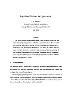
For every quantitative ¯eld with n classes, we use n ¡ 1 variables. The di®erence with former case is that these variables do not correspond to classes. They correspond instead to nested intervals, all of them having as initial point the smaller feasible value for that ¯eld, and as ¯nal point the identi¯ed breakpoints. Externally from the bigger nested interval it remains the 'out of range' class. This choice for variable association results, in our case, in shorter clauses. In fact, in most of edits appear similar intervals. They can therefore be expressed with one variable instead of more ones. If the quantitative ¯eld f has a value in one of the nested intervals [a,b] we put ®[a;b] = T rue. The other variable must be set accordingly, as illustrated below. The same holds for the other classes of the ¯eld, except for one, for instance the last one Cfn . When the ¯eld has a value in the 'out of range' class, we put all variables at F alse. Example 3.8. The ¯eld age is divided in 5 equivalence classes (see example 3.6). We therefore have 5-1 = 4 logical variables ®[0;14) , ®[0;18) , ®[0;26) , ®[0;120] , as illustrated below.

10

vage 2 [[0; 14)]

)

vage 2 [[14; 18)]

)

vage 2 [[18; 26)]

)

vage 2 [[26; 120]] ) vage 2 [blank]

)

½

½ ½ ½

½

®[0;14) = ®[0;18) = = ®[0;26) = ®[0;120] = T rue ®[0;14) = F alse ®[0;18) = ®[0;26) = ®[0;120] = T rue ®[0;14) = ®[0;18) = F alse ®[0;26) = ®[0;120] = T rue ®[0;14) = ®[0;18) = ®[0;26] = F alse ®[0;120] = T rue ®[0;14) = ®[0;18) = = ®[0;26] = ®[0;120] = F alse

We therefore have the following graphical representation of the nested intervals.

-∞

+∞ α 0,120 α 0,26 α 0,18 α 0,14 0

14 18 26

120

Figure 1: Logic variables used to encode the ¯eld age.

3.5

Encoding of edits as clauses

So far, every edit can be encoded in clauses by using the de¯ned variables. Every expressions (fi < relation > vfi ) can in fact be substituted by the corresponding logical variable, obtaining therefore a sequence of logic variables connected by logic operators, hence a logic formula. We are interested in producing clauses which are satis¯ed by consistent answers. Being edits the description of the error condition, we now need to negate the obtained logic formula. This negated logic formula can be then transformed in CNF format, by following simple syntactical logic rules. The so generated CNF formula is satis¯ed by every set of correct questionnaires answers, and are not satis¯ed by every set of inconsistent or out of range answer. With the particular edit structure considered,

11

every edit produces one and only one clause. However, in a general case, this could not hold, but the procedure works ¯ne as well. Example 3.9. Following the above example 3.1, the given edit is marital status = married ^ age < 14 By substituting the logical variables, we have the following logic formula ®[married] ^ ®[0;14) By negating it, and applying De Morgan's law, we obtain the following clause :®[married] _ :®[0;14)

3.6

Identi¯cation of congruency clauses

In addition to information given by edits, there is information which is not contained in edits, and that a human operator would consider obvious, but which must be provided to an automatic elaboration. In our case, we need to express that ¯elds must have one and only one value, and therefore other clauses, named congruency clauses, need to be added. By using n ¡ 1 variables for n equivalence classes, there is no need to add clauses expressing that we must have a value being in at least one class, because it does not exist a truth assignment for variables that doesn't verify this. Instead, it must be expressed that the value for a ¯eld must be in only one class. Considering the case of qualitative ¯elds (such as the example of marital status), we have the n variables corresponding to the n + 1 disjoint classes. The above condition becomes that only one variable can be true. This is imposed by adding clauses constituted by ¡ ¢ all the possible couples of negated variables. Their number is therefore n2 (number of combination of class 2 of n objects). Example 3.10. In the case of the qualitative ¯eld marital status, we have 5 ¡¢ variables, hence the congruency clauses are 52 = 10, as follows: :®[single] :®[single] :®[single] :®[single] :®[married] :®[married] :®[married] :®[separate] :®[separate] :®[divorced]

_ _ _ _ _ _ _ _ _ _

:®[married] :®[separate] :®[divorced] :®[widow] :®[separate] :®[divorced] :®[widow] :®[divorced] :®[widow] :®[widow]

Considering now the case of quantitative ¯elds (such as the example of age), we have n variables corresponding to n nested subsets. As observed above, we can have either 12

the case of a quantitative ¯eld divided into nested intervals of reals, or the case of a quantitative ¯eld divided into nested sets of integer numbers. We will discuss the procedure speaking about nested intervals, but, of course, the case of nested sets of integers is completely analogous. The congruency condition becomes that, if a variable ®[a1 ;b1 ] , corresponding to an interval [a1 ; b1 ], is T rue, also all the variables ®[a2 ;b2 ] ; ®[a3 ;b3 ] ; : : : ; corresponding to all the intervals [a2 ; b2 ]; [a3 ; b3 ]; : : : ; containing [a1 ; b1 ], must ¡ ¢be T rue. The above condition is imposed by adding (n ¡ 1) + (n ¡ 2) + : : : + 1 = n2 clauses expressing ®[a1 ;b1 ] ) ®[a2 ;b2 ] ; ®[a1 ;b1 ] ) ®[a3 ;b3 ] ; : : : ; ®[a2 ;b2 ] ) ®[a3 ;b3 ] ; : : : ;

Converting in CNF by applying elementary logic rules (®a ) ®b is equivalent to :®a _ ®b ), we obtain :®[a1 ;b1 ] _ ®[a2 ;b2 ] ; :®[a1 ;b1 ] _ ®[a3 ;b3 ] ; : : : ; :®[a2 ;b2 ] _ ®[a3 ;b3 ] ; : : : ; Example 3.11. In the case of the quantitative ¯eld age, we have¡ 4¢ variables corresponding to 4 nested subsets, hence the congruency clauses are 42 = 6, as follows: :®[0;14) _ ®[0;18) :®[0;14) _ ®[0;26) :®[0;14) _ ®[0;120] :®[0;18) _ ®[0;26) :®[0;18) _ ®[0;120] :®[0;26) _ ®[0;120] So far, given the set of edits, we have a set of m clauses, and, given the set of answers to a questionnaire, we have a truth assignment for the n logical variables. By construction, a record which does not activate any edit, will satisfy all the clauses, and a record which activates some edits will not satisfy the corresponding clauses. We therefore have that the truth assignment given by a record must satisfy all the clauses to be declared correct. We will hence consider the conjunction of all the clauses, that is a CNF formula E, and say, brie°y, that the questionnaire Q must satisfy E to be declared correct.

4

Edits Validation

As told, edits must be free from inconsistency (i.e. edits must not be in contradiction each other), and, preferably, from redundancy (i.e. do not contain edit which are logically implied from other edits). The test for contradictions and redundancies is very hard for a human operator, and impossible above a certain number of edits. On the other hand, when such test is automatically performed, it historically turns out to be very computationally demanding. A di®use approach follows the so-called 'Fellegi-Holt' methodology [11]. This consists in checking for contradiction and redundancy by generating all the (new) edits 13

which are implied by the given edits. The generation of all implied edits allows to check if the given edits imply some hidden rule that should not hold. Unfortunately, but predictably, the number of implied edits is exponential in the number of given edits. This is the main reason for which this methodology, although theoretically irreproachable, is recently recognized to be not applicable for many real-world problems. Edit representation by means of ¯rst-order logic was already proposed, for instance in [4]. This allows a formal and convenient description of the edit and the operations. However, something analogous to the generation of all implied edits must be performed in this case also. The computational complexity of the problem remains exponential. Being our proposal to perform edit validation in the case of real world problems, we must get rid of the generation of all implied edits. By means of a propositional logic representation, the problem of checking for inconsistency and redundancy can be formalized as follows.

4.1

Complete Inconsistency in the Set of Edits

When every possible set of answers to the questionnaire is declared incorrect, we have the situation called complete inconsistency of the set of edits. In fact, reminding that edits describe the inconsistent situation, let us consider the following example. Example 4.1. The following is a situation of Complete Inconsistency. This is, of course, a very simple and evident one. More complex ones, involving dozens of edits, are not so easily visible. Below every edit its meaning is explained. seaside house = no meaning: everybody must have a seaside house. mountain house = no meaning: everybody must have a mountain house. (seaside house = yes) ^ (mountain house = yes) meaning: it is not allowed to have both seaside and mountain house. Using these edits, every questionnaire fails the check, because it cannot exist any set of answers which appear consistent. Edits are always activated. In a large set of edits, or in a phase of edits updating performed by people di®erent from the original edit writers, the situation of complete inconsistency may occur. Claim 4.1. By encoding edits in clauses, complete inconsistency correspond to a CNF formula that cannot be satis¯ed, namely an unsatis¯able formula. Complete inconsistency can therefore be detected by checking the satis¯ability of the whole CNF formula.

14

Moreover, when having a complete inconsistency and in order to restore consistency, it would be very useful to know which are the inconsistent edits. This corresponds to selecting which part of the unsatis¯able CNF cause the unsolvability, i.e. a minimal unsatis¯able subformula (MUS) [7, 12, 18]. This could be done by means of the used SAT solver, which, in the case of unsatis¯able instances, is able to select a subset of clauses which are still unsatis¯able, and thus causes the unsatis¯ability of the whole instance [7]. Therefore, the inconsistent edits are the ones corresponding to such clauses, and should be changed (by the human adviser who writes the edits, of course). The usefulness of the individuation of such inconsistent subset of edits is easily understandable when thinking of the prospect of checking, for instance, a dozen of edits instead of one thousand.

4.2

Partial Inconsistency in the Set of Edits

More insidious because less easy to detect without an automatic procedure in a large set of edits is the situation of partial inconsistency of the set of edits. This happens when some questionnaires, which are correct, are declared erroneous, only due to a particular value vfy of a single ¯eld f. In the intentions of the edit writer, vfy was a feasible value for the ¯eld f . Due to an unfortunate edit combination, however, there is an hidden and unwanted implied edit which forbids the value vfy for the ¯eld f . vfy will be called a sentence value. When a correct questionnaire contains a sentence value, it is (erroneously) declared incorrect, due to edit's fault. For questionnaires not containing sentence values, partial inconsistency does not cause any problem. Let us consider indeed the following example. Example 4.2. The following is a situation of partial inconsistency. Below every edit its meaning is explained. (annual income ¸ 1000) ) (seaside house = no) meaning: if annual income is greater then or equal to 1000, then the subject must have a seaside house. (annual income ¸ 2000) ) (mountain house = no) meaning: if annual income is greater then or equal to 2000, then the subject must have a mountain house. (seaside house = yes) ^ (mountain house = yes) meaning: it is not allowed to have both seaside and mountain house. Using the above edits, every questionnaires where the subject has an annual income ¸ 2000 is declared erroneous, even if it should not. In fact, that answer necessarily activates the edits. Note that, for annual income < 2000, this partial inconsistence does not show any e®ect, and error detection proceeds in the correct way. The value 2000, (and any other greater value) is a sentence value for the ¯eld annual income. We can have more than one sentence value vfy forbidden by the same unwanted implied edit. The set of all values forbidden by an unwanted implied edit is in fact constituted 15

by the subset Sfj containing vfy , together with all other subsets belonging to the same equivalence class (see sec. 3). The logical variable corresponding to the equivalence class [Sfj ] will be called sentence variable ®fy for the ¯eld f . The set of all the values forbidden by one unwanted implied edit will be called sentence set Sfy . Sfy

[

=

Sfk

k: Sfk 2[Sfj ]; vfy 2Sfj

We will therefore say that we have partial inconsistency with regard to the set Sfy for the ¯eld f , or, equivalently, with regard to the variable ®yf for the ¯eld f . Note that we can have more unwanted implied edits forbidding more variables of the same ¯eld. In case of partial inconsistency, the CNF formula obtained from the edits is satis¯able. However, if for ¯eld f we have a sentence value, this corresponds to ¯xing the sentence variable ®yf to T rue. Claim 4.2. If we ¯x ®fy to T rue, and remove, as standard, satis¯ed clauses and all negated occurrence of that variable, the resulting formula becomes unsatis¯able. Basing on the above result, partial inconsistency with regard to any single variable ®k of the CNF formula can be detected by checking the satis¯ability of all the CNF formulae obtained by independently ¯xing ®k = T rue, for k = 1; : : : ; n. Partial inconsistency with respect to a single variable ®k , will be called ¯rst-level partial inconsistency. Partial inconsistency with respect to a couple of variables ®k and ®h , will be called second-level partial inconsistency, and so on. We don't check all levels, otherwise we could not get rid from the exponential complexity that a®ects other procedures. What we do is to check all ¯rst-level partial inconsistencies, and provide a tool that allows to check, if desired, higher-level partial inconsistencies. Note that neither 'Fellegi-Holt' methods check such partial inconsistencies, since they do dot lead to a complete contradiction when deriving all implied edits, and therefore are not automatically signaled. With 'Fellegi-Holt' methods, in fact, they could only be found by a (hypothetic) human inspector which examines every implied edit generated. Moreover, in order to restore consistency, the used SAT solver is still able to select a subset of clauses which are unsatis¯able, and thus causes the situation of partial inconsistency. Individuation of inconsistent edits can therefore be carried out also in the case of partial inconsistency.

4.3

Redundancy in the set of edits

Some edits could be logically implied by others, being therefore redundant. It would be obviously preferable if we could remove them, because decreasing the number of edits while maintaining the same power of inconsistency detection can simplify the whole process and make it less error prone.

16

Example 4.3. The following is a (very simpli¯ed) situation of edit redundancy. Below every edit its meaning is explained. (role = head of the house) ^ (annual income < 100) meaning: head of the house must have an annual income greater then or equal to 100. annual income < 100 meaning: everybody must have an annual income greater then or equal to 100. The ¯rst edit is clearly redundant. A SAT formulation is generally used to solve the problem of logical implication, i.e., given a set of statements S called axioms, to decide whether another statement s logically derives from them, in symbols S ) s. Representing statements S and s with clauses, we have S ) s if and only if S [ :s is an unsatis¯able formula [17, 19]. In our case this means: Claim 4.3. The clausal representation of an edit ej is implied by the clausal representation of a set of edits E if and only if the CNF formula obtained by E [ :ej is unsatis¯able. It can be consequently checked if an edit is redundant by removing its clausal representation ej from the CNF formula, by adding its negation :ej to the formula, and by testing if the resulting formula is unsatis¯able. The redundancy of every edit can be checked by independently applying to each one of them the above operation

5

Individuation of Erroneous Records

Once we have a valid set of edit rules, they are used to detect erroneous records, in our case questionnaires. A correct questionnaire will be indicated with Qr (right) and an erroneous one with Qw (wrong). By using the propositional logic representation, this trivially becomes the problem of checking if the truth assignment corresponding to each questionnaire Q satis¯es the CNF formula E obtained from the set of edits plus the congruency clauses. This operation can be performed with an extremely small computational e®ort. It results therefore suitable to check even a very large number of questionnaires.

6

The Problem of Imputation

After detection of erroneous records, if information collecting has no cost, we could just cancel erroneous records and collect new information until we have enough correct records. Since usually information collecting has a cost, we would like to use also the correct part of information contained in the erroneous records. This means changing the erroneous records in order to try to restore the unknown correct values. Such operation is called imputation. 17

We will call original data the unknown data that we would have if we had no errors, and original frequency distributions the unknown frequency distributions that we would have if we had no errors. We will correspondingly call original questionnaire Qo the questionnaire that we would have if we had no errors. In our case, therefore, given an erroneous questionnaire Qw , the imputation process consists in changing some of his values in order to obtain a corrected questionnaire Qc which satis¯es the formula E. Imputation should be done by keeping as much as possible the correct information contained in erroneous data. Two general principles should be followed [11]: ² To apply the minimum changes to erroneous data. ² To modify as less as possible the marginal and joint original frequency distribution of the data. The above principles frequently clash. We give an example to clarify this point. Example 6.1. Consider this case of error: someone whose age is 70 and marital status is married. The original questionnaire would be Qo = f ... age = 70, ... marital status = married, ... g However, the subject forgets to write the zero of 70 and writes 7. The questionnaire we actually have is Qw = f ... age = 7, ... marital status = married, ... g Such record is immediately detected as erroneous, since we have an edit which says 'if marital status is married, age must be ¸ 14'. Suppose that, in virtue of some procedure (presented below), we know that the errors is in the ¯eld age. We therefore want to correct the value of age. The point is how to correct that. Imagine in fact that we have many records which are in the above situation, in the sense that their original values for age were any value above 14, but the erroneous values we have on the questionnaire are all below 14. If we just try to correct age by changing it as less as possible, we put all of such values at 14, as follows. Qc = f ... age = 14, ... marital status = married, ... g The statistical distribution of the original age would therefore be remarkably altered, by having a wrong peak in 14. Note that, even if we try to correct age by choosing a random value above 14 which has the same frequency distribution of the age of married people (distribution obtained from the correct questionnaires) we could alterate the joint frequency distribution of the ¯eld age with respect to other ¯elds. To continue the example, imagine that our subject (who is 70 years old), has, for the ¯eld work, the value retired. Imagine that the random value used to correct age is 50 (quite plausible). We have:

18

Qc =f ... age = 50, ... marital status = married, ... work = retiredg We can observe that the original (unknown) joint frequency distribution of the two ¯elds age and work is altered. The same could happen for the other original joint frequency distributions. There are two main approaches to the above problem of imputation: the deterministic and the probabilistic one. Such approaches can sometimes be combined. Given an erroneous record, a deterministic imputation reconstruct the record with a deterministic procedure, renouncing to keep the original unknown joint frequency distributions. Note that errors can be stochastic or systematic. Stochastic errors are randomly introduced, and can therefore be unpredictable and have in general low or no correlation. Systematic errors consists in a repetition of the same error. This can be, for instance, due to some structural defect in the questionnaire. Deterministic methods are valid in the case of systematic errors, being in fact a systematic correction. Deterministic imputation just require a priori decisions, and therefore do not present speci¯c computational di±culties. A probabilistic imputation, on the contrary, for every erroneous record, tries to correct it by choosing new values which are not predetermined. The same erroneous records can therefore be corrected in more than one way. Such methods are generally preferred in the case of stochastic errors, because they assure a more uniform data correction, and can salvage the original frequency distributions. The drawback of probabilistic procedures usually is their computational burden.

6.1

Error Localization

A ¯rst problem arising when a questionnaire is declared erroneous, is to locate the error, namely to understand which are the erroneous ¯elds. We could assume that the erroneous ¯elds are the smallest set of ¯elds that, if changed, permit to restore consistency, in the sense of not activating the edits anymore. This assumption is based on the fact that, when error is something unintentional, the more likely event is that errors are the smaller number. This is coherent with the principle of minimum change. In addiction to the above, one can argue that some ¯elds can be more reliable than others. This means that the probability they are erroneous is lower. What is generally done is to give, for every ¯eld fi , a measure ri 2 IR+ of the reliability, which corresponds to a \preference" in keeping unchanged the value of ¯eld fi . We de¯ne the total cost of a correction as the sum of the reliabilities ri of the ¯elds to modify fiw . By calling W the set of the fiw , the cost of such correction is X c (W ) = ci i:fiw 2W

Therefore, the problem of error localization is the following. Given the erroneous questionnaire Qw and the CNF formula E to be satis¯ed, we want to ¯nd a set W of ¯elds fiw such that:

19

² The corrected questionnaire Qc satisfying E can be obtained from the erroneous one Qw by changing (only and all) the values of the fiw 2 W . ² The total cost of required changes c(W ) is minimum. We can in fact have more than one set of ¯elds whose imputation can restore consistency, and we are interested in the one which changes as few as possible Qw . As for the values to put in such ¯elds, two approaches are generally considered. One is to generate the imputed values by means of some (stochastic) function, although this could change the original unknown frequency distribution of the data (see example 6.1). The second is to use a donor questionnaire Qd .

6.2

Imputation through a Donor

A donor questionnaire Qd is a correct questionnaire which, according to some distance function d(Qw ; Qd ) 2 IR+ , is the nearest one to the erroneous questionnaire Qw we want to correct. Therefore, it represents a subject which has very similar characteristics. Given Qw and Qd , we simply copy the values of the ¯elds fiw that we need to change from the donor Qd to the erroneous Qw . This procedure is generally recognized to cause a low alteration of the original frequency distributions. Example 6.2. Consider this case of the error in example 6.1: someone whose age is 70 and marital status is married. The erroneous questionnaire we have is Qw = f ... age = 7, ... marital status = married, ... g Assume that the ¯eld marital status has a cost cmarital status = 8, and the ¯eld age has a cost cage = 3. This means that the answer to the ¯eld marital status is considered more reliable than the answer to the ¯eld age. We ¯nd that the set W of minimum cost is just the ¯eld fageg. We therefore want to perform the imputation of the ¯eld age. Assume that, if we consider the values of all the ¯elds of Qw , the subject appears to be an elderly man. Let therefore assume that, by searching for a correct questionnaire at minimum distance (considering all ¯elds) from Qw we ¯nd another elderly man: Qd = f ... age = 72, ... g We can now proceed with the imputation of the ¯eld age from the donor. This restores consistency. We obtain Qc =f ... age = 72, ... marital status = married, ... g Note that, in this case, the corrected questionnaire Qc is very similar to the original one Qo . This does not happen by chance, but is due to the mechanism of imputation trough a donor.

20

However, two problems arise from the use of a donor. The ¯rst is that, if we have not enough correct questionnaires to ¯nd a donor which is close to Qw , the imputed values can be not so similar to the original ones. The second is that, by using a donor, we are not guaranteed that the set of erroneous ¯elds of minimum cost W is enough to restore consistency of Qw . In fact, W is that set of ¯elds at minimum cost that can be changed to restore consistency, but the use of a donor does not let to change such ¯elds as much as we like. We could need to take more ¯elds from the donor, or we could need to take the ¯elds of another set W 0 6= W , before restoring consistency. However, we have the guarantee that, since the donor is a correct questionnaire, there exists in Qd at least one set of ¯elds whose values are able to restore consistency of Qw . The second problem is related to the ¯rst, since, having a very numerous set of correct questionnaires, the case when we need to copy from the donor a set of ¯elds di®erent from W before restoring consistency is rare. Moreover, the number of ¯elds we could need to add in this case is low. Consider the following (very rough) example. Example 6.3. We have an erroneous questionnaire Qw Qw = f ... age = 17, ... car = no, ... city of residence = aaa, ... ..., city of work = bbb, ... time to go to work = 20, ... g where the set of erroneous ¯elds of minimum cost is f age, car g, with a total cost of 5.5. Imagine we could restore consistency only if, for these two ¯elds, we have age¸ 18 and car = yes. Searching for a donor, however, we ¯nd Qd such that Qw = f ... age = 16, ... car = yes, ... city of residence = aaa, ... ... city of work = aaa, ... time to go to work = 20, ... g If we proceed with imputation of the two selected ¯elds f age, car g, we do not restore consistency at all. We need to choose a di®erent set of ¯elds. In this case, imagine that the imputation of the set of ¯elds f age, city of work g, with a total cost of c = 6, restores consistency. By taking them from the donor, we obtain: Qw = f ... age = 17, car = yes, city of residence = aaa, ... ... city of work = aaa, ... time to go to work = 20, ... g Therefore, the problem of imputation trough a donor is the following. Given the erroneous questionnaire Qw , the donor questionnaire Qd , and the CNF formula E to be satis¯ed, we want to ¯nd a set D of ¯elds fid such that: ² The corrected questionnaire Qc satisfying E can be obtained from the erroneous one Qw by copying from the donor Qd (only and all) the values of the fid 2 D. ² The total cost of the correction c(D) is minimum. In this case also we can have more than one set of ¯elds whose imputation can restore consistency, and we are interested in the one which changes as few as possible Qw . Due to the motivations noted above, we have that c(W ) · c(D). Variants to the above procedure are possible (the number of donors, how to choose a donor), but the spirit of the imputation trough a donor remains the same. 21

7

A Set Covering Formulation

We can observe that, in both the cases of the use of an imputation function or of the use of a donor, we actually want to ¯nd a set of changes of minimum cost such as we can restore consistency, i.e. satisfy the CNF formula E. The above problem can be modeled as a weighted set covering problem [21]. Given a ground set S of n elements si , and a collection A of m subsets Aj of S (for example, the collection may consists of all subsets of size k · n), the set covering problem is the problem of taking a set of elements si of minimum cardinality such as we have at least one element for every Aj . A little more general problem is the following. Given a ground set S of n elements si , each one with a cost ci 2 IR+ , and a collection A of m sets Aj of elements of S, the weighted set covering problem is the problem of taking the set of elements si of minimum total weight such as we have at least one element for every Aj . Note that the ¯rst problem is a special case of the second when all the costs are 1. Let aj be the incidence vector of Aj , i.e. a vector in f0; 1gn whose i-th component j ai is 1 if si 2 Aj , and 0 if si 62 Aj . Consider a vector of variables x 2 f0; 1gn which is the incidence vector of the set of the elements si we take. We can give the following mathematical model for the above problems. min s: t:

n X

i=1 n X i=1

ci xi aji xi ¸ 1

j = 1:::m

(1)

x 2 f0; 1gn The set covering problem is a classical combinatorial optimization problem, with binary variables which assume values in f0,1g. It is of great relevance for modeling and solving a variety of problems arising form many practical ¯elds. It is known to be NP-complete [13]. Set covering formulations are used, for instance, in the ¯elds of telecommunications, transportation, facility location, crew scheduling, and, in general, when the problem has the structure of a set of something that must be covered. In order to work in the ¯eld of binary optimization, we now transform the logic variables ®i taking values in fT rue; F alseg into binary variables xi taking values in f0,1g. The di®erence is only formal, and the conversion is straightforward. While the operations de¯ned on the logical variables where f^; _; : : :g, the operations de¯ned on the binary variables are f+; ¡; : : :g In particular, a positive literal ®i corresponds to a binary variable xi , and a negative literal :®i corresponds to a negated binary variable x ¹i . Note that x ¹i and xi must have opposite values, just like :®i and ®i . A set of answers to a questionnaire, which corresponded to a truth assignment in fT rue; F alsegn , will now correspond to a binary vector in f0; 1gn . The following propositional clause cj (®i _ ::: _ ®j _ :®k _ ::: _ :®n )

22

will now correspond to the following linear inequality, by de¯ning the set A¼ of the logical variables which appear positive in cj , and the set Aº of the logical variables which appear negative in cj , and the corresponding incidence vectors a¼ and aº n X i=1

a¼i xi +

n X i=1

aºi x ¹i ¸ 1

For each clause we have an inequality of the above type. If we write all of them, we obtain that the logic formula E that the truth assignment must satisfy (®i1 _ ::: _ ®j1 _ :®k1 _ ::: _ :®n1 ) ^ : : : ^ (®im _ ::: _ ®jm _ :®km _ ::: _ :®nm ) corresponds now to the following system of linear inequalities that must satisfy. 0 ¼ 10 x 1 0 º 10 x ¹1 1 a1;1 ::: a¼1;n a1;1 ::: aº1;n B .. .. C + @ @ AB A ::: ::: @ . A @ . a¼m;1 ::: a¼m;n aºm;1 ::: aºm;n xn x ¹n

the binary vector 1 1 C B .. C A¸@ . A 1 1

0

Example 7.1. Suppose that the truth assignment corresponding to the (correct) questionnaire Q is f®1 = F alse; ®2 = F alse; ®3 = T rueg and that the logic formula E used to detect erroneous questionnaires is (:®1 _ ®2 _ :®3 ) ^ (:®1 _ :®2 ) ^ (®2 _ ®3 ) The binary vector corresponding to the questionnaire Q is fx1 = 0; x2 = 0; x3 = 1g and the system of 0 0 @ 0 0

linear inequalities corresponding to E is 10 1 0 10 1 0 1 1 0 x1 1 0 1 x ¹1 1 0 0 A @ x2 A + @ 1 1 0 A @ x ¹2 A ¸ @ 1 A 1 1 x3 0 0 0 x ¹3 1

Moreover, in order to take into account the reliability of every ¯eld, we estimate a vector of n costs fc1 ; : : : ; cn g corresponding to the variables f®1 ; : : : ; ®n g. We pay ci when we change ®i . Note that, since every ¯eld corresponds to more variables, such costs are not directly the reliability of a ¯eld. On the other hand, an estimation of an individual cost for every variable allows more subtile evaluations. We can now model the imputation problems as follows.

23

7.1

Error Localization

In the case of error localization, we have ² The binary vector e = fe1 ; : : : ; en g 2 f0; 1gn corresponding to the erroneous questionnaire Qw . ² The binary variables x = fx1 ; : : : ; xn g 2 f0; 1gn and their complements x ¹ = f¹ x1 ; : : : ; x ¹n g 2 f0; 1gn , with the coupling constraints xi + x ¹i = 1. The variables x represent the truth assignment corresponding to the corrected questionnaire Qc that we want to ¯nd. ² The system of linear inequalities A¼ x+ Aº x ¹ ¸ 1, with A¼ ; Aº 2 f0; 1gm£n , that e does not satisfy. We know that such system has binary solutions, since E is satis¯able and has more than one solution. ² The vector c0 = fc1 ; : : : ; cn g 2 IRn+ of costs that we pay for changing e. We pay ci for changing ei . We introduce furthermore a vector of binary variables y = fy1 ; : : : ; yn g 2 f0; 1gn representing the changes we introduce in e. We have ½ 1 if we change ei yi = 0 if we keep ei According to the principle of the minimum change, we want to change the erroneous questionnaire Qw minimizing the total cost of the changes. This can be expressed as min

yi 2f0;1g

n X

ci yi =

i=1

min c0 y

y2f0;1gn

(2)

We want a corrected questionnaire Qc which satis¯es the system of inequalities A¼ x + Aº x ¹¸1

(3)

A key issue is that there is a relation between variables y and x (and consequently x ¹). This depends on the values of e, as follows: ½ xi (= 1 ¡ x ¹i ) if ei = 0 yi = (4) 1 ¡ xi (= x ¹i ) if ei = 1 In fact, when ei = 0, to keep it unchanged means to put xi = 0. Since we do not change, yi = 0. On the contrary, to change it means to put xi = 1. Since we change, yi = 1. Altogether, yi = xi . When, instead, ei = 1, to keep it unchanged means to put xi = 1. Since we do not change, yi = 0. On the contrary, to change it means to put xi = 0. Since we change, yi = 1. Altogether, yi = 1 ¡ xi .

24

By using the above result, we can express the problem of error localization with the following formulation. Our objective function (2) becomes min

xi ;¹ xi 2f0;1g

n n X X (1 ¡ ei )ci xi + ei ci x ¹i i=1

(5)

i=1

Subject to the following constraints A¼ x + Aº x ¹¸1 xi + x ¹i = 1 x; x ¹ 2 f0; 1gn We will call satis¯ability constraints the ¯rst kind of constraints, deriving in fact from the propositional satis¯ability problem. We will call coupling constraints the second kind of constraint. The third kind are the binary constraints over the variables. The above formulation is a set covering problem, as de¯ned in (1).

7.2

Imputation through a Donor

The case of imputation through a donor is very similar. We have ² The binary vector e = fe1 ; : : : ; en g 2 f0; 1gn corresponding to the erroneous questionnaire Qw . ² The binary vector d = fd1 ; : : : ; dn g 2 f0; 1gn corresponding to the donor questionnaire Qd . ² The binary variables x = fx1 ; : : : ; xn g 2 f0; 1gn and their complements x ¹ = f¹ x1 ; : : : ; x ¹n g 2 f0; 1gn , with the coupling constraints xi + x ¹i = 0. x corresponds to the corrected questionnaire Qc that we want to ¯nd. ² The system of linear inequalities A¼ x+ Aº x ¹ ¸ 1, with A¼ ; Aº 2 f0; 1gm£n , that e does not satisfy. We know that such system has binary solutions, since E is satis¯able and has more than one solution. ² The vector c0 = fc1 ; : : : ; cn g 2 IRn+ of costs that we pay for changing e. We pay ci for changing ei . We use, as before, a vector of binary variables y = fy1 ; : : : ; yn g 2 f0; 1gn representing the elements that we copy from d to e. We have ½ 1 if we copy di in ei yi = 0 if we keep ei According to the principle of the minimum change, we want to change the erroneous questionnaire Qw minimizing the total cost of the changes. This can be expressed as min

yi 2f0;1g

n X

ci yi =

i=1

25

min c0 y

y2f0;1gn

(6)

We want a corrected questionnaire Qc which satis¯es the system of inequalities A¼ x + Aº x ¹¸1

(7)

In this case also, there is a relation between variables y and x (and consequently x ¹). This depends on the values of e and d, as follows: 8 ¹i ) if ei = 0 and di = 1 < xi (= 1 ¡ x yi = 1 ¡ xi (= x ¹i ) if ei = 1 and di = 0 (8) : 0 if ei = di

In fact, when ei = 0 and di = 1, not to copy the element means to put xi = 0. Since we do not change, yi = 0. On the contrary, to copy the element means to put xi = 1. Since we change, yi = 1. Altogether, yi = xi . When, instead, ei = 1 and di = 0, not to copy the element means to put xi = 1. Since we do not change, yi = 0. On the contrary, to copy the element means to put xi = 0. Since we change, yi = 1. Altogether, yi = 1 ¡ xi . Finally, when ei = di , we have no gain from copying the element, and therefore we do not change. Altogether, yi = 0. By using the above result, we can express the problem of imputation through a donor with the following formulation. Our objective function (2) becomes min

xi ;¹ xi 2f0;1g

n n X X (1 ¡ ei )di ci xi + ei (1 ¡ di )ci x ¹i i=1

(9)

i=1

Subject to the following constraints A¼ x + Aº x ¹¸1 xi + x ¹i = 1 x; x ¹ 2 f0; 1gn Similarly with the former case, we will call satis¯ability constraints the ¯rst kind of constraints, deriving in fact from the propositional satis¯ability problem. We will call coupling constraints the second kind of constraint. The third kind are the binary constraints over the variables. Also the above formulation is a set covering problem, as de¯ned in (1). The above problems are therefore solved with the volume algorithm [2, 3], which is a recently proposed and very e®ective combinatorial optimization algorithm.

8

Implementation

We ¯rst implemented a series of procedures in order perform the automatic conversion of the set of edits into a CNF formula. After that, in virtue of modeling our problems as classical optimization problems, we could take advantage of the huge amount of research done in the ¯elds of satis¯ability and set covering solvers. The satis¯ability problems are solved by means of an enumeration procedure called Adaptive Core Search (ACS)[7]. Such solver, in fact, turns out to be a very e®ective 26

one, as proved in [6]. Moreover, in the case of unsatis¯able instances, ACS is able to select a subset of clauses which are still unsatis¯able, and thus cause the unsatis¯ability. This is a key feature in our case, since, in the cases of inconsistencies, we need to correct them, and this is possible only when the set of 'culprit' edits can be located. All the edits validation process was implemented to run sequentially, and interactively asking, for every inconsistence of redundancy found, whether stop the process and let the edit-writer mend the set of edit, or ignore it and continue. The set covering problems are then solved by implementing the Volume Algorithm [2, 3]. This very e®ective procedure recently developed by Barahona is an extension of the subgradient algorithm, with the key feature is that is able to produce primal as well dual solutions. This gives a fast method for producing approximated solutions for large scale linear programs. We added a simple heuristic in order to obtain an integer solution to our set covering problem, together with a bound allowing to verify the quality of such solution. Such heuristic consists in a rounding of the fractionary solution. Rounding is deterministic (and just cuts at 1/2) for some fractionary values, while being probabilistic for particular combinations of fractionary values. The choice of the Volume Algorithm made possible to solve problems whose size is not solvable by a commercial Branch-and-Bound solver (Xpress).

9

Results

We performed the process of edits validation and data imputation in the case of a Census of Population. The set of edits are kindly provided by the Italian National Statistic Institute (ISTAT). In the course of this work, we actually did several tests, by considering di®erent sets of edits. They ranged from 100 to 400 edits. Such procedure were considered to be quite representative of how a real census proceeds. All the described procedure were implemented in C++ and tested on a Pentium II 450MHz PC under MS Windows Operating System. In this census, the data of every family were collected by using a single questionnaire. Individuals were identi¯ed by number, and edits were originally written with this structure. Edits have been rewritten identifying individuals by roles, which are: head of the family, consort, father of head, mother of head, brother/sister of head, son, additional son, father in law, mother in law, daughter in law, son in law, grandchild. This was done by taking obviously care of maintaining the exact meaning of the original edits. This choice produces a more compact set of edits, while its congruency and redundancy properties remain the same. Being a questionnaire for an entire family, we can have similar edits repeated for every member of the family. Edit replication, called explosion, is the ¯rst automatically performed step. It is then applied the procedure of automatic conversion of edits into clauses. The implemented software takes in input a ¯le containing the set of edits, a ¯le containing a description of the ¯elds, a ¯le containing lists of all feasible values of qualitative ¯elds, and a ¯le containing the list of family roles. The procedure identi¯es logical 27

variables, according to outlined procedure, and gives in output a ¯le listing the used logical variables, with their meaning, and the CNF formula which encodes the set of edits. The generation of the logic formula is not a costing operation. For the problem we deal with, resulting formulas range from 315 variables and 650 clauses to 450 variables and 1100 clauses. Since this kind of problems are solved quite easily, in order to test the limits of the procedure, we moreover considered arti¯cially generated satis¯ability instances of bigger size. They ranged from 1000 variables and 5000 clauses to 15000 variables and 75000 clauses.

9.1

Edit Validation

Our algorithm begins with solving the satis¯ability problem for the CNF formula, in order to detect complete inconsistency for the set of edits. After this, in order to detect all 1-level partial inconsistency, the procedure goes ahead ¯xing in turn every variable to T rue and then all the variables of every ¯eld to F alse, and solving at every step the resulting SAT instance. The test for redundancies is then made by negating in turn every clauses, and solving at every step the resulting SAT instance. Hence, for every instance with n variables and m clauses, the implemented algorithm solves in cascade about 1 + n + n=10 + m satis¯ability problems of non trivial size. Although such problems do not reveal to be structurally hard, the computational burden is substantial. Therefore, there is the need of an e±cient SAT solver. We used ACS, a recently proposed and very e±cient SAT solver, which uses an enumeration scheme with a new adaptive technique [7]. In the following tables we report number of variables (n) and number of clauses (m) of the propositional CNF formula, the number of problem we had to solve (# of problems), and total time for solving all of them (time). In table 1 we report results on formulas which are the encoding of the real census edits. In table 2 we report results on arti¯cially generated formulas. n 315 350 380 402 425 450

m 650 710 806 884 960 1103

# of problems 975 1090 1219 1321 1428 1599

time 0.99 1.35 1.72 2.21 2.52 3.24

Table 1: Results of the edit validation procedure on real sets of edits . Our solver is able, in the case of an unsatis¯able instance, of providing a set of clauses which cause the unsolvability, in order to understand were is the inconsistency. In the analyzed set of real edits, which were supposed to be error free, a partial inconsistency was found, that was due to one of the edit concerning divorced people, as explained below. Married people must be at least 14 years old, and a divorce procedure takes at

28

least four years. It results that divorced people must be at least 18 years old. There was an edit representing this, and it was erroneously written (marital status 2 fsingle; married; separate; widowg) ^ (age < 18) The correct edit should have been the following. (marital status = divorced) ^ (age < 18) Such problem could of course cause errors during the phase of individuation of erroneous records. By checking for redundancy, several clauses resulted redundant, hence the corresponding edits are already implied by the rest of the edits. Further tests, performed after deliberately introduction of inconsistency or redundancy in the set of edits, lead in the totality of the cases to their detection. n 1000 3000 5000 8000 10000 15000

m 5000 15000 25000 40000 50000 75000

# of problems 6101 18301 30501 48801 61001 91501

time 15 415 1908 7843 16889 >36000

Table 2: Results of the edit validation procedure on arti¯cially generated sets of edits . In the case of arti¯cially generated instances, partial inconsistencies and redundancies were found. Their description is not signi¯cative, being arti¯cially generated problems. They were used in order to understand which size of problems the proposed procedure is able to treat. Afterwards, detection of erroneous questionnaires answers have been performed, as a trivial task. It proceeds converting the set of answers in values for the logical variables, and simply testing if such truth assignment satis¯es the CNF formula obtained from the edits.

9.2

Data Imputation

The procedure for data imputation was tested on simulated questionnaires, and by using the two sets of real edits and the arti¯cially generated ones. We considered both the problems of error localization and imputation through a donor. For each set of edits we considered various simulated erroneous answers. In particular, we considered the percentage of activated edits for the erroneous answer. Since errors are usually a small part of the answers, we realistically considered small edit activation percentages (1%, 2%, 3%, etc.). Note that a set of edit corresponding to n logic variables and m clauses corresponds here to a set covering formulation with 2n variables and m satis¯ability constraints plus n coupling constraints, altogether m + n. 29

We solved the set covering formulation by means of a set covering solver based on the Volume Algorithm. Moreover, since this is an approximate procedure, we compared its results with the commercial Branch-and-Bound solver Xpress. In some cases of high error percentage, the solver based on the Volume Algorithm could not ¯nd a feasible integer solution. In those cases we reported \-". We report a di®erent table for each instance, with time and solution value in all the above cases. Problems of error localization follow. Time error

VA

0:5% 0:9% 1:3% 2:4% 5:0%

0.01 0.10 0.10 0.14 0.22

Value B&B 3.18 3.18 3.45 2.86 3.50

VA 43.0 221.6 328.4 729.5 300.8

B&B 43.0 221.6 328.4 729.5 300.8

Table 3: Error localization procedure on a real set of edits. The set covering instance has 400 var. and 1400 const. Time error 0:4% 0:7% 1:0% 1:6% 2:5% 3:5%

VA 0.04 0.10 0.11 0.16 0.20 0.23

B&B 1.91 1.91 2.54 1.90 2.50 2.98

Value VA B&B 58.6 58.6 108.6 108.6 140.1 140.1 506.7 506.7 1490.1 1490.1 2330.8 2330.8

Table 4: Error localization procedure on a real set of edits. The set covering instance has 480 var. and 1880 const. Time error 0:7% 1:5% 2:1% 3:6% 6:7%

VA 0.51 0.68 0.55 0.98 1.00

B&B 2.44 3.02 3.32 3.73 4.40

Value VA B&B 463.2 463.2 394.5 394.5 612.5 612.5 1254.8 1254.8 2341.2 2341.2

Table 5: Error localization procedure on a real set of edits. The set covering instance has 800 var. and 3200 const. From the above tables, we can observe that real problems are solved e±ciently both by VA and B&B. Surprisingly, VA reaches in all cases the optimal integer solution, given by the B&B. Times are very small in both cases, and they increase with error percentage (and, of course, with the size of the problem). In addition, we tested the procedure on arti¯cially generated instances, corresponding to the arti¯cially generated satis¯ability instance considered in the case of edit validation.

30

Time

Value

error

VA

B&B

0:4% 1:0% 1:1% 1:8% 4:3%

0.66 1.30 0.73 1.92 3.65

87.90 81.88 97.71 109.05 87.16

VA 329.4 1010.4 952.9 1982.0 5549.8

B&B 329.4 1010.4 952.9 1982.0 5549.8

Table 6: Error localization procedure on an arti¯cially generated set of edits. The set covering instance has 2000 var. and 6000 const. Time error 0:5% 0:8% 1:0% 2:1% 4:0%

VA 11.60 4.75 5.10 4.76 11.63

B&B 3813.4 3477.7 2796.9 4117.2 3595.0

Value VA B&B 1273.7 1273.6 2266.1 2266.1 3604.3 3604.3 6064.2 6064.2 1544.7 1544.6

Table 7: Error localization procedure on an arti¯cially generated set of edits. The set covering instance has 6000 var. and 18000 const. Time error

VA

B&B

0:5% 0:7% 1:3% 1:7% 3:0%

8.27 10.87 11.80 28.58 41.35

18837.8 19210.5 19493.6 18506.6 17000.3

Value VA B&B 2018.1 3817.1 6409.2 9673.7 21742.5

2018.1 3817.1 6409.2 9673.7 21742.4

Table 8: Error localization procedure on an arti¯cially generated set of edits. The set covering instance has 10000 var. and 30000 const. Time error

VA

B&B

0:4% 0:9% 1:3% 2:0% 4:0%

9.16 20.36 40.64 66.60 73.54

>21600 >21600 >21600 >21600 >21600

Value VA B&B 3058.4 6897.7 11682.9 20113.0 37069.1

-

Table 9: Error localization procedure on an arti¯cially generated set of edits. The set covering instance has 16000 var. and 48000 const.

31

Time error

VA

B&B

0:5% 0:8% 1:3% 2:1% 3:6%

44.44 30.61 31.42 83.41 74.64

>21600 >21600 >21600 >21600 >21600

Value VA B&B 5135.4 8640.5 14466.7 23093.7 39448.2

-

Table 10: Error localization procedure on an arti¯cially generated set of edits. The set covering instance has 20000 var. and 60000 const.

error 0:4% 0:9% 1:3% 2:0% 4:0%

Time VA B&B 35.74 >21600 47.33 >21600 107.97 >21600 94.42 >21600 186.92 >21600

Value VA B&B 6754.7 12751.3 20135.4 31063.6 66847.4 -

Table 11: Error localization procedure on an arti¯cially generated set of edits. The set covering instance has 30000 var. and 90000 const. From the above tables, we can observe that arti¯cially generated problems of very big size are all solved by VA, while B&B cannot solve the bigger instance within the time limit of 6 hours. However, we begin to notice that the solution found by VA is not optimal, although the di®erence is numerically negligible. Further occasional tests with higher error percentage shows that VA does not increase running time, but the heuristic is not able to ¯nd a feasible integer solution, hence we have no solution, while B&B would reach such solution but in an a prohibitive amount of time. In the case of a donor, we considered a simulated donor, which is a correct solution very similar to the erroneous one. Results both for real and arti¯cially generated sets of edits follow. Time error

VA

0:5% 0:9% 1:3% 2:4% 5:0%

0.04 0.04 0.04 0.04 0.03

Value B&B 0.01 0.01 0.01 0.04 0.03

VA 43.4 227.5 348.7 726.6 365.8

B&B 43.4 227.5 348.7 726.6 365.8

Table 12: Imputation through a donor on a real set of edits. The set covering instance has 400 var. and 1400 const.

32

Time error

VA

0:4% 0:7% 1:0% 1:6% 2:5% 3:5%

0.04 0.06 0.06 0.06 0.07 0.06

Value B&B 0.02 0.02 0.02 0.02 0.02 0.03

VA

B&B

63.6 144.7 264.5 643.5 1774.3 2369.9

63.6 144.7 264.5 643.1 1774.1 2369.5

Table 13: Imputation through a donor on a real set of edits. The set covering instance has 480 var. and 1880 const. Time error 0:7% 1:5% 2:1% 3:6% 6:7%

VA 0.08 0.08 0.08 0.08 0.10

B&B 0.04 0.06 0.06 0.07 0.07

Value VA B&B 280.1 280.1 453.5 453.1 655.4 655.0 1378.0 1378.0 2455.1 2455.0

Table 14: Imputation through a donor on a real set of edits. The set covering instance has 800 var. and 3200 const. Time error

VA

0:4% 1:0% 1:1% 1:8% 4:3%

0.26 0.10 0.04 0.08 -

Value B&B 0.01 0.31 0.01 0.31 0.20

VA

B&B

331.2 1015.2 952.9 1997.1 -

331.2 1015.1 952.9 1997.1 5592.2

Table 15: Imputation through a donor on an arti¯cially generated set of edits. The set covering instance has 2000 var. and 6000 const. Time error

VA

0:5% 0:8% 1:0% 2:1% 4:0%

0.17 0.17 0.70 0.38 0.65

Value B&B 0.30 0.10 0.30 0.30 0.30

VA 1291.6 2305.4 3660.1 6124.0 1585.7

B&B 1291.4 2305.4 3660.1 6123.1 1585.0

Table 16: Imputation through a donor on an arti¯cially generated set of edits. The set covering instance has 6000 var. and 18000 const.

33

Time error

VA

0:5% 0:7% 1:3% 1:7% 3:0%

1.01 1.30 1.40 1.60 1.05

B&B 0.6 0.6 0.3 0.6 0.3

Value VA B&B 2120.1 3877.7 6411.7 9690.1 21823.1

2118.9 3877.2 6411.7 9690.1 21802.4

Table 17: Imputation through a donor on an arti¯cially generated set of edits. The set covering instance has 10000 var. and 30000 const. Time error

VA

0:4% 0:9% 1:3% 2:0% 4:0%

0.44 4.59 0.86 -

B&B 0.6 0.6 0.8 0.6 0.9

Value VA B&B 3064.2 6899.7 11702.9 -

3064.2 6899.6 11698.3 19814.5 36496.7

Table 18: Imputation through a donor on an arti¯cially generated set of edits. The set covering instance has 16000 var. and 48000 const. Time error 0:5% 0:8% 1:3% 2:1% 3:6%

VA 2.85 3.28 3.41 3.82 -

B&B 0.9 0.9 0.9 0.9 0.9

Value VA B&B 5139.1 5139.0 8688.0 8687.0 14500.4 14478.5 23411.7 23072.0 44026.8

Table 19: Imputation through a donor on an arti¯cially generated set of edits. The set covering instance has 20000 var. and 60000 const. Time error 0:4% 0:9% 1:3% 2:0% 4:0%

VA 3.58 3.22 0.97 2.89 -

B&B 1.27 1.27 0.9 1.27 1.59

Value VA B&B 6788.1 6788.1 12760.0 12759.5 20140.1 20140.0 31258.1 31082.2 - 67764.94

Table 20: Imputation through a donor on an arti¯cially generated set of edits. The set covering instance has 30000 var. and 90000 const. From the above tables, we can observe that all problems are solved is very short times. B&B is always able to ¯nd a solution within seconds. VA, on the other hand, is not able to ¯nd a solution when error increases too much. Moreover, the solution found by VA is not optimal in several cases, although the di®erence is very small. This can be explained by noting that, in the problem of imputation through a donor, some variables are ¯xed to the value thy have in the donor. This results in a 34

problem with much less variables but with a high error percentage. In this conditions the preferable solution method is a complete one, such like B&B. To summarize the results, VA outperform B&B in the case of error localization in very big instances with a moderate error. On the contrary, in the case of smaller problems with higher error (not realistic), or in some cases of imputation through a donor, B&B is more reliable.

10

Conclusions

A binary encoding is the more direct and e®ective representation both for records and for the set of edit rules in a process of data collecting. It allows to automatically detect inconsistencies and redundancies in the set of edit rules. Erroneous records detection is carried out with an inexpensive procedure. The proposed encoding allows, moreover, to automatically perform error localization and data imputation. The related computational problems are overcome by using state-of-the-art solvers. Approached real problems have been solved in extremely short times. Arti¯cially generated problems are e®ectively solved until sizes which are orders-of-magnitude larger than the above real-world problems. Hence, noteworthily qualitative improvements in a general process of data collecting are made possible. The implemented software is tested in the case of a real Population Census. Edits are kindly provided by the Italian National Statistic Institute (ISTAT). Results are extremely encouraging. Acknowledgments. The authors would like to thank Sonia Benzi, Francisco Barahona, Fabiana Birarelli, Carlo Mannino, Alessandra Reale.

References [1] M. Bankier. Experience with the New Imputation Methodology used in the 1996 Canadian Census with Extensions for future Census. UN/ECE Work Session on Statistical Data Editing, Working Paper n.24, Rome, Italy, 2-4 June 1999. [2] F. Barahona and R. Anbil. The Volume Algorithm: producing primal solutions with a subgradient method. IBM Research Report RC21103, 1998. [3] F. Barahona and F. Chudak. Near-optimal solutions to large scale facility location problems. IBM Research Report RC21606, 1999. [4] G. Barcaroli. Un approccio logico formale al problema del controllo e della correzione dei dati statistici. Quaderni di Ricerca ISTAT n.9/1993. [5] E. Boros, P.L. Hammer, T. Ibaraki and A. Kogan. Logical analysis of numerical data. Mathematical Programming, 79:163{190, 1997. [6] R. Bruni and A. Sassano. CLAS: a Complete Learning Algorithm for Satis¯ability. Dipartimento di Informatica e Sistemistica, Universitµ a di Roma \La Sapienza" , Technical Report 6-99, 1999. [7] R. Bruni and A. Sassano. Finding Minimal Unsatis¯able Subformulae in Satis¯ability Instances. in proc. of 6th Internat. Conf. on Principles and Practice of Constraint Programming, Lecture notes in Computer Science 1894, Springer-Verlag, 500{505, 2000.

35

[8] M. Davis, G. Logemann, and D. Loveland. A machine program for theorem-proving. Comm. Assoc. for Comput. Mach., 5:394{397, 1962. [9] M. Davis and H. Putnam. A computing procedure for quanti¯cation theory. Jour. Assoc. for Comput. Mach., 7:201{215, 1960. [10] O. Dubois, P. Andre, Y. Boufkhad, and J. Carlier. SAT versus UNSAT. DIMACS Series in Discrete Mathematics and Theoretical Computer Science, 26:415{436, 1996. [11] P. Fellegi and D. Holt. A Systematic Approach to Automatic edit and Imputation. Journal of the American Statistical Association, 17:35{71(353), 1976. [12] H. Fleischner and S. Szeider. Polynomial-time Recognition of Mimimal Unsatis¯able Formulas with Fixed Clause-Variable Di®erence. submitted to Elsevier Preprint. 1999. [13] M.R. Garey and D.S. Johnson. Computers and Intractability: A Guide to the Theory of NP-Completeness. W.H. Freeman and Company, San Francisco, 1979. [14] M.R. Genesereth and N.J. Nillson. Logical Foundation of Arti¯cial Intelligence. Morgan Kaufmann, 1987. [15] F. Harche, J.N. Hooker, and G.L. Thompson. A computational study of Satis¯ability Algorithms for Propositional Logic. ORSA Journal on Computing, 6:423{435, 1994. [16] R.E. Jeroslow and J. Wang. Solving Propositional Satis¯ability Problems. Annals of Mathematics and AI, 1:167{187, 1990. [17] R. Kowalski. Logic for Problem solving. North Holland, 1978. [18] O. Kullmann. An application of matroid theory to the SAT problem. ECCC TR00-018, February 2000. [19] D.W. Loveland. Automated Theorem Proving: a Logical Basis. North Holland, 1978. [20] M. Masselli, M. Signore, F. Panizon. Il sistema di controllo della qualit¶ a dei dati. Manuale di tecniche di indagine ISTAT, vol. 6, 1992. [21] G.L. Nemhauser and L.A. Wolsey. Integer and Combinatorial Optimization. J. Wiley, New York, 1988. [22] C. Poirier. A Functional Evaluation of Edit and Imputation Tools. UN/ECE Work Session on Statistical Data Editing, Working Paper n.12, Rome, Italy, 2-4 June 1999. [23] J.R. Quinlan. Induction of decision trees. Machine Learning, 1:81{106, 1986. [24] A. Van Gelder and Y.K. Tsuji. Satis¯ability testing with more reasoning and less guessing. DIMACS Series in Discrete Mathematics and Theoretical Computer Science, 26:559{586, 1996. [25] W.E. Winkler. State of Statistical Data Editing and current Research Problems. UN/ECE Work Session on Statistical Data Editing, Working Paper n.29, Rome, Italy, 2-4 June 1999.

36