Published by the University of Newcastle upon Tyne,. School of ... In order to alleviate this problem, Petri net analysis techniques based on causal partial.
School of Computing Science, University of Newcastle upon Tyne
Logic Synthesis Avoiding State Space Explosion Khomenko, V., Koutny, M. and Yakovlev, A.
Technical Report Series CS-TR-813
August 2003
c Copyright 2003 University of Newcastle upon Tyne Published by the University of Newcastle upon Tyne, School of Computing Science, Claremont Tower, Claremont Road, Newcastle upon Tyne, NE1 7RU, UK.
Logic Synthesis Avoiding State Space Explosion Victor Khomenko1 , Maciej Koutny1 , and Alex Yakovlev2 1 School of Computing Science 2 School of Electrical, Electronic and Computer Engineering University of Newcastle upon Tyne NE1 7RU, United Kingdom {Victor.Khomenko, Maciej.Koutny, Alex.Yakovlev}@ncl.ac.uk
Abstract. The behaviour of asynchronous circuits is often described by Signal Transition Graphs (STGs), which are Petri nets whose transitions are interpreted as rising and falling edges of signals. One of the crucial problems in the synthesis of such circuits is deriving equations for logic gates implementing each output signal of the circuit. This is usually done using reachability graphs. In this paper, we avoid constructing the reachability graph of an STG, which can lead to state space explosion, and instead use only the information about causality and structural conflicts between the events involved in a finite and complete prefix of its unfolding. We propose an efficient algorithm for logic synthesis based on the Incremental Boolean Satisfiability (SAT) approach. Following the description of our method, we present some problem-specific optimization rules. Experimental results show that this technique leads not only to huge memory savings when compared with the methods based on reachability graphs, but also to significant speedups in many cases. Keywords: logic synthesis, asynchronous circuits, self-timed circuits, Petri nets, signal transition graphs, STG, SAT, net unfoldings, partial order techniques.
1
Introduction
Signal Transition Graphs (STGs) is a formalism widely used for describing the behaviour of asynchronous control circuits. Typically, they are used as a specification language for the synthesis of such circuits [3,6,27]. STGs are a class of interpreted Petri nets, in which transitions are labelled with the names of rising and falling edges of circuit signals. Circuit synthesis based on STGs involves: (i) checking the necessary and sufficient conditions for the STG’s implementability as a logic circuit; (ii) modifying, if necessary, the initial STG to make it implementable; and (iii) finding appropriate boolean covers for the next-state functions of output and internal signals and obtaining them in the form of boolean equations for the logic gates of the circuit (logic synthesis). One of the commonly used STG-based synthesis tools, Petrify [5,6], performs all of these steps automatically, after first constructing the reachability graph (in the form of a BDD [1]) of the initial STG specification. A vivid example of its use was the design of many circuits for the Amulet-3 microprocessor. Since popularity of this tool is steadily growing, it is very likely that STGs and Petri nets will increasingly be seen as an intermediate (back-end) notation for the design of large controllers. While the state-based approach is relatively simple and well-studied, the issue of computational complexity for highly concurrent STGs is quite serious due to the state space explosion problem. This puts practical bounds on the size of control circuits that can be synthesized using such techniques, which are often restrictive, especially if the STG models are not constructed manually by a designer but rather generated automatically from high-level hardware descriptions. In order to alleviate this problem, Petri net analysis techniques based on causal partial order semantics, in the form of Petri net unfoldings, had been applied for circuit synthesis. In [13, 14], we proposed a solution for one of the subproblems, central to the implementability analysis in step (i), viz. checking the Complete State Coding (CSC) condition [3]. In essence, this problem consists in detecting the state encoding conflicts, which occur when semantically
2
V.Khomenko, M.Koutny, and A. Yakovlev
different reachable states have the same binary encoding. We showed that the notion of an encoding conflict can be characterized in terms of either feasibility of a system of integer constraints [13] or satisfiability of a boolean formula (SAT) [14]. Those algorithms achieved significant speedups compared with methods based on reachability graphs, and provided a basis for the framework for resolution of encoding conflicts (step (ii) above) described in [18], which used the set of pairs of configurations representing encoding conflicts produced by the algorithm as an input. However, those techniques would have limited practical impact if it was necessary to construct the reachability graph in the later stages of the design cycle for asynchronous circuits. To address this concern, we show in this paper how Petri net unfolding techniques can be used for deriving equations for logic gates of the circuit (step (iii) above). This essentially completes the design cycle for complex-gate synthesis that does not involve building reachability graphs at any stage. Our experiments have shown that the proposed method has significant advantage both in memory consumption and in execution time compared with the existing state space based methods.
2
Basic definitions
In this section, we first present basic definitions concerning Petri nets and STGs, and then recall notions related to net unfoldings (see also [4–6, 9, 12, 15, 16, 19, 20, 23, 24, 27]) and boolean satisfiability (see also [21, 28]). 2.1
Petri nets df
A net is a triple N = (P, T, F ) such that P and T are disjoint sets of respectively places and transitions (collectively referred to as nodes), and F ⊆ (P × T ) ∪ (T × P ) is a flow df relation. A marking of N is a multiset M of places, i.e., M : P → N = {0, 1, 2, . . .}. We adopt the standard rules about representing nets as directed graphs, viz. places are represented as circles, transitions as rectangles, the flow relation by arcs, and markings are shown by placing tokens within circles. In addition, the following short-hand notation is used: a transition can be connected directly to another transition if the place ‘in the middle of the arc’ has exactly one incoming and one outgoing arc (see, e.g., Figure 1(a)). If this hidden place contained a df token, it is drawn directly on the arc. As usual, we will denote • z = {y | (y, z) ∈ F } and S df df df S z • = {y | (z, y) ∈ F }, for all z ∈ P ∪ T , and • Z = z∈Z • z and Z • = z∈Z z • , for all Z ⊆ P ∪ T . We will assume that • t 6= ∅ 6= t• , for every t ∈ T . df A net system is a pair Σ = (N, M0 ) comprising a finite net N = (P, T, F ) and an (initial) marking M0 . A transition t ∈ T is enabled at a marking M , denoted M [ti, if for every s ∈ • t, df M (s) ≥ 1. Such a transition can be executed, leading to a marking M 0 given by M 0 = M −• t+t• , where ‘−’ and ‘+’ stand for the multiset difference and sum, respectively. We denote this by M [tiM 0 or M [iM 0 if the identity of the transition is irrelevant. The set of reachable markings of Σ is the smallest (w.r.t. ⊆) set [M0 i containing M0 and such that if M ∈ [M0 i and M [iM 0 then M 0 ∈ [M0 i. For a finite sequence of transitions σ = t1 . . . tk , we denote M [σiM 0 if there are markings M0 , . . . , Mk such that M0 = M , Mk = M 0 and Mi−1 [ti iMi , for i = 1, . . . , k. A net system Σ is k-bounded if, for every reachable marking M and every place p ∈ P , M (p) ≤ k, and safe if it is 1-bounded. Moreover, Σ is bounded if it is k-bounded for some k ∈ N. One can show that the set [M0 i is finite iff Σ is bounded. 2.2
Signal Transition Graphs df
A Signal Transition Graph (STG) is a triple Γ = (Σ, Z, λ) such that Σ = (N, M0 ) is a net df system, Z is a finite set of signals, generating a finite alphabet Z ± = Z × {+, −} of signal ± transition labels, and λ : T → Z is a labelling function. The signal transition labels are of the
Logic Synthesis Avoiding State Space Explosion
dsr+
dtack−
dsr+
dtack−
lds+
3
00100
10000 00000
ldtack−
ldtack− lds+
ldtack− dsr+
dtack− 01100
11000
10010
01000 ldtack+ d−
lds−
lds−
lds−
ldtack+
lds− dsr+
dtack−
ldtack−
M 00 11010
01110 01010
M0
d+
d− dtack+
dsr− dsr−
dtack+
d+
11010
01111
(a)
11111
11011
(b) inputs: dsr , ldtack ; outputs: dtack , lds, d
Fig. 1. An STG modelling a simplified VME bus controller (a) and its state graph with a CSC conflict between two states (b). The order of signals in the binary encodings is: dsr , ldtack , dtack , lds, d .
form z + or z − , and denote a transition of a signal z ∈ Z from 0 to 1 (rising edge), or from 1 to 0 (falling edge), respectively. Signal transitions are associated with the actions which change the value of a particular signal. We will use the notation z ± to denote a transition of signal z if we are not particularly interested in its direction. Γ inherits the operational semantics of its underlying net system Σ, including the notions of transition enabling and execution, reachable markings, and firing sequences. df 0 ) ∈ {0, 1}|Z| , We associate with the initial marking of Γ a binary vector v 0 = (v10 , . . . , v|Z| 0 where each vi corresponds to the signal zi ∈ Z. Moreover, with any finite sequence of trandf σ sitions σ we associate an integer signal change vector v σ = (v1σ , v2σ , . . . , v|Z| ) ∈ Z|Z| , so that + σ each vi is the difference between the number of the occurrences of zi –labelled and zi− –labelled transitions in σ. Γ is consistent 1 if, for every reachable marking M , all firing sequences σ from M0 to M have the same encoding vector Code(M ) equal to v 0 + v σ , and this vector is binary, i.e., Code(M ) ∈ {0, 1}|Z| . Such a property guarantees that, for every signal z ∈ Z, the STG satisfies the following two conditions: (i) the first occurrence of z in the labelling of any firing sequence of Γ starting from M0 has the same sign (either rising of falling); and (ii) the transitions corresponding to the rising and falling edges of z alternate in any firing sequence of Γ . In this paper it is assumed that all the STGs considered are consistent.2 We will denote by Code z (M ) the component of Code(M ) corresponding to a signal z ∈ Z. The consistency can be enforced syntactically, by adding to the STG, for each signal z ∈ Z, a pair of complementary places, p0z and p1z , tracing the value of z as follows. Each z + –labelled transition has p0z in its preset and p1z in its postset, and each z − –labelled transition has p1z in its preset and p0z in its postset. Exactly one of these two places is marked at the initial state, accordingly to the initial value of signal z. One can show that at any reachable state of an STG augmented with such places, p0z (respectively, p1z ) is marked iff the value of z is 0 1
2
This is a somewhat simplified notion of consistency; see [23] for a more elaborated one. Our approach works also for the notion presented there. The consistency of an STG can easily be checked during the process of building its finite and complete prefix [23].
4
V.Khomenko, M.Koutny, and A. Yakovlev
(respectively, 1). Thus, if a transition labelled by z + (respectively, z − ) is enabled then the value of z is 0 (respectively, 1), which in turn guarantees the consistency of the augmented STG. Such a transformation can be done completely automatically. For a consistent STG, it does not restrict the behaviour and yields an STG with an isomorphic state graph (see below); for a non-consistent STG, the transformation restricts the behaviour and may lead to (new) deadlocks. In what follows, we assume that the tracing places are present in the STG, and df df df denote PZ0 = {p0z | z ∈ Z}, PZ1 = {p1z | z ∈ Z}, and PZ = PZ0 ∪ PZ1 . df df The state graph of Γ is a tuple SG Γ = (S, A, M0 , Code) such that: S = [M0 i is the set of df t states; A = {M → M 0 | M ∈ [M0 i ∧ M [tiM 0 } is the set of state transitions; M0 is the initial state; and Code : S → {0, 1}|Z| is the state assignment function, as defined above for markings. The signals in Z are partitioned into input signals, ZI , and output signals, ZO (the latter may also include internal signals). Input signals are assumed to be generated by the environment, while output signals are produced by the logic gates of the circuit. Logic synthesis derives for each output signal z ∈ ZO a boolean next-state function Nxt z df defined for every reachable state M of Γ as follows: Nxt z (M ) = 0 if Code z (M ) = 0 and no z + –labelled transition is enabled at M , or Code z (M ) = 1 and a z − –labelled transition is df enabled at M ; and Nxt z (M ) = 1 if Code z (M ) = 1 and no z − –labelled transition is enabled at M , or Code z (M ) = 0 and a z + –labelled transition is enabled at M . Moreover, the value of this function must be determined without ambiguity by the encoding of each reachable state, i.e., Nxt z (M ) should be a function of Code(M ) rather than of M , i.e., Nxt z (M ) = Fz (Code(M )) for some function Fz : {0, 1}Z → {0, 1} (Fz will eventually be implemented as a logic gate). To capture this, let M 0 and M 00 be two distinct states of SG Γ , z ∈ ZO and X ⊆ Z. M 0 and M 00 are in Complete State Coding conflict for z w.r.t. X (CSC zX conflict) if Code x (M 0 ) = Code x (M 00 ) for all x ∈ X and Nxt z (M 0 ) 6= Nxt z (M 00 ). Γ satisfies the CSC property for z (CSC z property) if no two states of SG Γ are in CSC zZ conflict. Γ satisfies the CSC property if it satisfies the CSC z property for each z ∈ ZO .3 X is a support of z ∈ ZO if no two states of Γ are in CSC zX conflict. In such a case the value of Nxt z at each state M of SG Γ is determined without ambiguity by the encoding of M restricted to X. A support X of z ∈ ZO is minimal if no set Y ⊂ X is a support of z. In general, a signal can have several distinct minimal supports. Moreover, for each signal z ∈ ZO we define Out z (M ) to be 1 if there exists a transition t enabled at M such that λ(t) = z ± ; and 0 otherwise. An example of an STG for a data read operation in a simple VME bus controller (a standard STG benchmark, see, e.g., [6]) is shown in Figure 1(a). It satisfies the CSC dtack property (with the minimal support {d }), but not the CSC d and CSC lds properties. Part (b) of this figure illustrates a CSC conflict for these signals between two different states, M 0 and M 00 , that have the same encoding, 11010, but Nxt d (M 0 ) = 1 6= Nxt d (M 00 ) = 0 and Nxt lds (M 0 ) = 1 6= Nxt lds (M 00 ) = 0. This means that the values of Fd (1, 1, 0, 1, 0) and Flds (1, 1, 0, 1, 0) are illdefined (they should be 1 according to the state M 0 and 0 according to the state M 00 ), and thus these signals are not implementable as a logic gates. To cope with this, an additional signal, csc, helping to resolve this CSC conflict is added to the STG, e.g., as shown in Figure 2(a,b). (Note that the circuit has to implement this new signal, and so for the purpose of logic synthesis it is regarded as output, though it is invisible to the environment.) Now the equations implementing each output signal can be obtained by applying boolean minimization to the truth table shown in Figure 2(c). The first column of this table lists the encodings of all the states of SG Γ , while the other columns give the corresponding values of the next-state functions for all the output signals. Note that not all possible encodings are present in the first column because the number of reachable states (16) is smaller than the number of possible encodings (2 6 = 64). This means that the missing encodings form the ‘don’t care’ set, i.e., the values of the functions at these encodings are not important and can be chosen arbitrarily (boolean minimization procedures 3
This definition, though different in form from the conventional one (see, e.g., [13, 14]), is equivalent to it due to the fact that Nxt z (M 0 ) = Nxt z (M 00 ) for all z ∈ ZO iff the sets of output signals enabled at M 0 and M 00 are the same, provided that Code(M 0 ) = Code(M 00 ).
Logic Synthesis Avoiding State Space Explosion
dtack−
dsr+
csc+
dsr+
dtack−
lds+
csc+
001000
100001 000000
ldtack−
ldtack−
100000 lds+
ldtack− dsr+
dtack− 011000
100101 010000
ldtack+
d− lds−
lds−
lds−
lds−
ldtack+
dsr+
dtack−
ldtack−
110000
011100
110101 010100
110100 d+
d− csc− csc−
dtack+
dsr−
d+
011110
(a)
5
dtack+
dsr− 011111
111111
110111
(b)
inputs: dsr , ldtack ; outputs: dtack , lds, d ; internal: csc Code(M ) Nxt dtack (M ) Nxt lds (M ) Nxt d (M ) Nxt csc (M ) 001000 0 0 0 0 000000 0 0 0 0 100000 0 0 0 1 100001 0 1 0 1 011000 0 0 0 0 010000 0 0 0 0 110000 0 0 0 0 100101 0 1 0 1 011100 0 0 0 0 010100 0 0 0 0 110100 0 0 0 0 110101 0 1 1 1 011110 1 1 0 0 011111 1 1 1 0 111111 1 1 1 1 110111 1 1 1 1 Expression: d d ∨ csc csc ∧ ldtack dsr ∧ (¬ldtack ∨ csc) (c) Fig. 2. An STG (a) where the CSC conflict has been resolved by adding a new signal, csc; its state graph (b); and the truth table for the output signals (c) with the last row showing the result of boolean minimization. The order of signals in the binary encodings is: dsr , ldtack , dtack , lds, d , csc.
can exploit this to reduce the complexity of the resulting boolean expression). The last row of the table gives the result of boolean minimization, viz. the expressions computed by logic gates implementing the output signals of the circuit. This essentially completes the standard complex gate synthesis procedure based on state graphs. 2.3
Branching processes
Two nodes of a net N = (P, T, F ), y and y 0 , are in structural conflict, denoted by y#y 0 , if there are distinct transitions t, t0 ∈ T such that • t ∩ • t0 6= ∅ and (t, y) and (t0 , y 0 ) are in the reflexive transitive closure of the flow relation F , denoted by ¹. A node y is in structural self-conflict if y#y.
6
V.Khomenko, M.Koutny, and A. Yakovlev df
An occurrence net is a net ON = (B, E, G) where B is the set of conditions (places), E is the set of events (transitions) and G is a flow relation. It is assumed that: ON is acyclic (i.e., ¹ is a partial order); for every b ∈ B, |• b| ≤ 1; for every y ∈ B ∪ E, ¬(y#y) and there are finitely many y 0 such that y 0 ≺ y, where ≺ denotes the irreflexive transitive closure of G. Min(ON ) will denote the minimal elements of B ∪ E with respect to ¹. The relation ≺ is the causality relation. Two nodes are concurrent, denoted y co y 0 , if neither y#y 0 nor y ¹ y 0 nor y 0 ¹ y. A homomorphism from an occurrence net ON to a net system Σ is a mapping h : B ∪ E → S ∪ T such that: h(B) ⊆ S and h(E) ⊆ T (conditions are mapped to places, and events to transitions); for all e ∈ E, the restriction of h to • e is a bijection between • e and • h(e) and the restriction of h to e• is a bijection between e• and h(e)• (transition environments are preserved); the restriction of h to Min(ON ) is a bijection between Min(ON ) and M0 (minimal conditions correspond to the initial marking); and for all e, f ∈ E, if • e = • f and h(e) = h(f ) then e = f (there is no redundancy). df A branching process of Σ is a quadruple π = (B, E, G, h) such that (B, E, G) is an occurrence net and h is a homomorphism from it to Σ. A branching process π 0 = (B 0 , E 0 , G0 , h0 ) of Σ is a prefix of a branching process π = (B, E, G, h), denoted π 0 v π, if (B 0 , E 0 , G0 ) is a subnet of (B, E, G) such that: if e ∈ E 0 and (b, e) ∈ G or (e, b) ∈ G then b ∈ B 0 ; if b ∈ B 0 and (e, b) ∈ G then e ∈ E 0 ; and h0 is the restriction of h to B 0 ∪ E 0 . For each Σ there exists a unique (up to isomorphism) maximal (w.r.t. v) branching process, called the unfolding of Σ (it is infinite whenever Σ has an infinite execution). 2.4
Configurations and cuts
A configuration of an occurrence net ON is a set of events C such that for all e, f ∈ C, ¬(e#f ) df and, for every e ∈ C, f ≺ e implies f ∈ C. The configuration [e] = {f | f ¹ e} is called the df local configuration of e ∈ E, and hei = [e] \ {e} denotes the set of causal predecessors of e. A cut is a maximal (w.r.t. ⊆) set of conditions B 0 such that b co b0 , for all distinct b, b0 ∈ B 0 . Every marking reachable from Min(ON ) is a cut. df Let C be a finite configuration of a branching process π. Then Cut(C) = (Min(ON ) ∪ C • ) \ • C is a cut; moreover, the multiset of places h(Cut(C)) is a reachable marking of Σ, denoted Mark (C). A marking M of Σ is represented in π if the latter contains a finite configuration C such that M = Mark (C). Every marking represented in π is reachable, and every reachable marking is represented in the unfolding of Σ. A branching process π = (B, E, G, h) of Σ is complete if there is a set Ecut ⊆ E of cut-off events such that for every reachable marking M of Σ there exist a finite configuration C of π such that C ∩ Ecut = ∅ and M = Mark (C), and for every transition t enabled by M , there is an event e 6∈ C in π such that h(e) = t and C ∪ {e} is a configuration (e may be a cut-off event).4 Although, in general, an unfolding is infinite, for every bounded net system Σ one can construct a finite complete prefix of the unfolding of Σ, by choosing an appropriate set E cut of cut-off events, beyond which the unfolding is not generated. A branching process of an STG Γ = (Σ, Z, λ) is a branching process of Σ augmented with an additional labelling of its events, λ ◦ h : E → Z ± . One can easily check the consistency of Γ , once its finite and complete prefix has been built [23]. We also extend the functions Code, Code z , Nxt z , and Out z to finite configurations of the df df branching process of Γ as follows: Code(C) = Code(Mark (C)), Code z (C) = Code z (Mark (C)), df df Nxt z (C) = Nxt z (Mark (C)), and Out z (C) = Out z (Mark (C)). 4
This notion of completeness differs from the one given in [9], which does not mention cut-off events, and hence is not appropriate for algorithms making use of them. Having said that, one can show that the unfolding algorithm proposed in [9] builds prefixes which are complete not only in the sense of the definition given in [9], but also in the stronger sense assumed here.
Logic Synthesis Avoiding State Space Explosion
2.5
7
Boolean satisfiability
The boolean satisfiability (SAT) problem consists in finding a satisfying assignment, i.e., a mapping Var → {0, 1} defined on the set of variables Var occurring in a given boolean expression ϕ such that ϕ evaluates to 1. (Note that we identify the booleans false and true with integers 0 and 1, respectively, provided that this does not create confusion.) This expression is often assumed to be given in the conjunctive normal form (CNF) ϕ=
n _ ^
l,
i=1 l∈Li
i.e., it is represented as a conjunction of clauses, which are disjunctions of literals, each literal l being either a variable or the negation of a variable. It is assumed that no two literals in the same clause correspond to the same variable. In order to solve a boolean satisfiability problem, SAT solvers perform exhaustive search assigning the values 0 or 1 to the variables. To reduce the search space, they use various heuristics (see, e.g., [28] for a brief overview). An almost universally used one is the Boolean Constraint Propagation (BCP) rule, which tells that if all but one literals occurring in some clause have the value 0 then in order to satisfy the clause the remaining literal must have the value 1. This rule is applied iteratively, until no more variables can be assigned, on each step of the search. If at some point all the literals in some clause have the value 0 then the built partial assignment cannot be a part of any satisfying assignment, and the solver backtracks. Some of the leading SAT solvers, e.g., zChaff [21], can be used in the incremental mode, i.e., after solving a particular SAT instance the user can slightly change it (e.g., by adding and/or removing a small number of clauses) and execute the solver again. This is often much more efficient than solving these related instances as independent problems, because on the subsequent runs the solver can use some of the useful information (e.g., learnt clauses, see [28]) collected so far. In particular, such an approach can be used to compute projections of assignments satisfying a given formula, as described in sequel. Projecting satisfying assignments Let V ⊆ Var be a non-empty set of variables occurring in a formula ϕ, and Proj ϕ V be the set of all restricted assignments (or projections) A| V such that A is a satisfying assignment of ϕ. Using the incremental SAT approach it is possible to compute Proj ϕ V , as follows. Step Step Step Step Step Step
0: 1: 2: 3: 4: 5:
A = ∅. Run the SAT solver for ϕ. If ϕ is unsatisfiable then return A and terminate. Add A|V to A, where A is the satisfying W assignment found W in Step 1. Modify ϕ by appending a new clause v∈V ∧A(v)=1 ¬v ∨ v∈V ∧A(v)=0 v. Go back to Step 1.
Note that the procedure is correct since it terminates (as Step 4 eliminates at least one satisfying assignment, viz. the A found in Step 1) and returns Proj ϕ V (as Step 4 eliminates only those satisfying assignments A0 which have the same restriction A0 |V = A|V ). Suppose now that we are interested in finding only the minimal elements of Proj ϕ V , assuming that A|V ≤ A0 |V if A|V (v) ≤ A0 |V (v), for all v ∈ V . The above procedure can then be modified by changing Step 4 to: W Step 4’: Modify ϕ by appending a new clause v∈V ∧A(v)=1 ¬v.
Moreover, before terminating, an additional pass over the elements stored in A is made in order to eliminate any non-minimal projections. The modified procedure works since Step 4’ eliminates at least one satisfying assignment, viz. the A found in Step 1 (notice that if the all-zeros is the minimal element of Proj ϕ V then
8
V.Khomenko, M.Koutny, and A. Yakovlev
Step 4’ produces an unsatisfiable formula). Moreover, Step 4’ never eliminates any minimal element of Proj ϕ V other than A|V which has already been stored in A. Similarly, if we were interested in finding all the maximal elements of Proj ϕ V , then one could change Step 4 to: W Step 4”: Modify ϕ by appending a new clause v∈V ∧A(v)=0 v.
And, before terminating, an additional pass over the elements stored in A would be made in order to eliminate any non-maximal projections. It is worth noting that the iterative procedure is usually fast on the initial iterations as the formula ϕ is typically easily satisfiable, but it may become harder towards the end of its run. Note that a similar computation could be implemented using Binary Decision Diagrams (BDDs) [1], by eliminating quantifiers from ∃(Var\V )ϕ and then computing the solutions of the resulting formula. However, in practice, V is a small set (it corresponds to the inputs of a logic gate computing an output signal), and so such an approach would have to eliminate too many quantifiers, while the approach based on the incremental SAT benefits from this.
3
Logic synthesis based on unfolding prefixes
Although the process of logic synthesis described in Section 2 is straightforward, it suffers from the state space explosion problem due to the necessity of constructing the entire state graph of the STG. In this section, we describe an approach based on unfolding prefixes rather than state graphs. It has been noted it [13, 14] that in practice such prefixes are often much smaller than the corresponding state spaces. This can be explained by the fact that practical STGs usually contain a lot of concurrency but relatively few choices, and thus the prefixes are in many cases not much bigger then the STGs themselves. As a result, unfolding-based methods had clear advantage over the BDD-based techniques both in terms of memory usage and running time. 3.1
Outline of the proposed method
In [14], the CSC conflict detection problem was solved by reducing it to SAT. More precisely, given a finite and complete prefix of an STG’s unfolding, one can build a formula CSC which is satisfiable iff there is a CSC conflict. In this paper, we modify that construction in the way described below. We assume a given consistent STG satisfying the CSC property, and consider in turn each output signal z ∈ ZO . The starting point of the proposed approach is to consider the set N SUPP z of all sets of signals which are non-supports of z. Within the boolean formula CSC z , which we are going df to construct, non-supports are represented by variables nsupp = {nsuppx | x ∈ Z}, and, for a given assignment A, the set of signals X = {x | A(nsuppx ) = 1} is identified with the projection z A|nsupp . The key property of CSC z is that N SUPP z = Proj CSC nsupp , and so it is possible to use the z incremental SAT approach to compute N SUPP . However, for our purposes it is enough to df compute the maximal non-supports N SUPP zmax = max⊆ N SUPP z which can then be used for computing the set SUPP zmin = min⊆ {X ⊆ Z | X 6⊆ X 0 , for all X 0 ∈ N SUPP zmax } df
of all the minimal supports of z (another incremental SAT run will be needed for this). SUPP zmin captures the set of all possible supports of z, in the sense that any support is an extension of some minimal support, and vice versa, any extension of any minimal support is a support. However, the simplest equation is usually obtained for some minimal support, and this approach was adopted in our experiments. Yet, this is not a limitation of our method as one can also explore some or all of the non-minimal supports, which can be advantageous, e.g., for small circuits and/or when the synthesis time is not of paramount importance (this would sometimes
Logic Synthesis Avoiding State Space Explosion
9
allow to find a simpler equation). And vice versa, not all minimal supports have to be explored: if some minimal support has many more signals compared with another one, the corresponding equation will almost certainly be more complicated, and so too large supports can safely be discarded. Thus, as usual, there is a trade-off between the execution time and the degree of design space exploration, and our method allows one to choose an acceptable compromise. Typically, several ‘most promising’ supports are selected, the equations expressing Nxt z as a function of signals in these supports are obtained (as described below), and the simplest among them is implemented as a logic gate. Suppose now that X is a support of z already chosen. In order to derive an equation expressing Nxt z as a function of the signals in X, we build a boolean formula EQN X which has a variable codex for each signal x ∈ X and is satisfiable iff these variables can be assigned values in such a way that there is a reachable state M such that Code x (M ) = codex , for all x ∈ X. Now, using the incremental SAT approach one can compute the projection of the set of reachable encodings onto X (differentiating the stored solutions according to the value of Nxt z (M )), and feed the result to a boolean minimizer. To summarize, the proposed method is executed separately for each signal z ∈ Z O and has three main stages: (I) computing the set N SUPP zmax of maximal non-supports of z; (II) computing the set SUPP zmin of minimal supports of z; and (III) deriving an equation for a chosen support X of z. In the sequel, we describe each of these three stages in more detail. It should be noted that the size of the truth table for boolean minimization and the the number of times a SAT solver is executed in our method can be exponential in the number of signals in the support. Thus, it is crucial for the performance of the proposed algorithm that the support of each signal is relatively small. However, in practice it is anyway difficult to implement as an atomic logic gate a boolean expression depending on more than, say, eight variables. (Atomic behaviour of logic gates is essential for the speed-independence of the circuit, and a violation of this requirement can lead to hazards [3, 6].) This means that if an output signal has only ‘large’ supports then the specification must be changed (e.g., by adding new internal signals) to introduce ‘smaller’ supports. Such transformations are related to the technology mapping step in the design cycle for asynchronous circuits (see, e.g., [6]); we do not consider them in this paper. 3.2
Computing maximal non-supports
Suppose that we want to compute the set of all maximal non-supports of a signal z ∈ Z O . At the level of a branching process, a CSC zX conflict can be represented as an unordered conflict pair of configurations hC 0 , C 00 i whose final states are in CSC zX conflict, as shown in Figure 3. We adopt the following naming conventions. The variable names are in the lower case and names of formulae are in the upper case. Names with a single prime (e.g., conf 0e and CON F 0 ) are related to C 0 , and ones with a double prime (e.g., conf 00e ) are related to C 00 . If there is no prime then the name is related to both C 0 and C 00 . If a formula name has a single prime then the formula does not contain occurrences of variables with double primes, and the counterpart double prime formula can be obtained from it by adding another prime to every variable with a single prime. The subscript of a variable points to which element of the STG or the prefix the variable is related, e.g., conf 0e and conf 00e are both related to the event e of the prefix. By a variable without a subscript we denote the list of all variables for all possible values of the subscript, e.g., conf 0 will denote the list of variables conf 0e , where e runs over the set E \ Ecut . The following boolean variables will be used in the proposed translation (Figure 3 shows the values of these variables for the depicted conflict pair of configurations): – For each event e ∈ E \ Ecut , we create two boolean variables, conf 0e and conf 00e , tracing whether e ∈ C 0 and e ∈ C 00 , respectively. – For each signal x ∈ Z, we create two boolean variables, code0x and code00x , tracing the the values of Code x (C 0 ) and Code x (C 00 ) respectively, and a variable nsuppx indicating whether x belongs to a non-support.
10
V.Khomenko, M.Koutny, and A. Yakovlev
dsr+
csc+
lds+
ldtack+
d+
dtack+
dsr−
csc−
d−
e1
e2
e3
e4
e5
e6
e7
e8
e9
dtack−
dsr+
e10
e12 csc+
e14 cut-off
C
0
C
conf 0 = 1111000000000 en0 = 00001000000000 code0 = 110101
00
nsupp = 110000
e11
e13
lds−
ldtack−
conf 00 = 1111111111110 en00 = 00000000000010 code00 = 110000
Fig. 3. An unfolding prefix of the STG shown in Figure 2(a) illustrating a CSC csc {dsr ,ldtack } conflict between configurations C 0 and C 00 . Note that e14 is not enabled by C 00 (since e13 6∈ C 00 ), and thus Nxt csc (C 0 ) = 1 6= Nxt csc (C 00 ) = 0. The order of signals in the binary encodings is: dsr , ldtack , dtack , lds, d , csc.
• such that h(b) ∈ PZ1 , we create two boolean variables, cut0b – For each condition b ∈ B \ Ecut 00 and cutb , tracing whether b ∈ Cut(C 0 ) and b ∈ Cut(C 00 ) respectively. – For each event e ∈ E labelled by z, we create two boolean variables, en0e and en00e , tracing whether e is ‘enabled’ by C 0 and C 00 respectively. Note that unlike conf 0 and conf 00 , such variables are also created for the cut-off events. z
CSC = As already mentioned, our aim is to build a boolean formula CSC z such that Proj nsupp z N SUPP , i.e., after assigning arbitrary values to the variables nsupp, the resulting formula df is satisfiable iff there is a CSC zX conflict, where X = {x | nsuppx = 1}. Figure 3 shows the satisfying assignment (except the variables cut0 and cut00 ) corresponding to the CSC zX conflict depicted there. The target formula CSC z will be the conjunction of constraints described below.
Configuration constraints The role of first two constraints, CON F 0 and CON F 00 , is to ensure that C 0 and C 00 are both legal configurations of the prefix (not just arbitrary sets of events). CON F 0 is defined as the conjunction of the following formulae: ^
^
(conf 0e ⇒ conf 0f )
e∈E\Ecut f ∈• (• e)
and ^
^
¬(conf 0e ∧ conf 0f ) ,
e∈E\Ecut f ∈Ee df
where Ee = ((• e)• \ {e}) \ Ecut . The former formula ensures that C 0 is downward closed w.r.t. ¹, i.e., if e ∈ C 0 then its immediate predecessors are also in C 0 . The latter one ensures that C 0 contains no structural conflicts. (One should be careful to avoid duplication of clauses when generating this formula.) Note that one can shorten this formulae by replacing • (• e) by max¹ • (• e) and Ee by min¹ Ee . CON F 00 is defined similarly. CON F 0 and CON F 00 can be transformed into the CNF by applying the rules x ⇒ y ≡ ¬x∨y and ¬(x ∧ y) ≡ ¬x ∨ ¬y.
Logic Synthesis Avoiding State Space Explosion
11
Encoding constraint The role of this constraint is to ensure that Code x (C 0 ) = Code x (C 00 ) whenever nsuppx = 1. To build a formula establishing the value code0x of each signal x ∈ Z at the final state of C 0 , we observe that code0x = 1 iff p1x ∈ Mark (C 0 ), i.e., iff b ∈ Cut(C 0 ) for some p1x –labelled condition b (note that the places in PZ cannot contain more than one token). The latter can be captured by the constraint: _ ^ cut0b ) , (code0x ⇐⇒ x∈Z
b∈Bx
• | h(b) = p1x }. We then define CODE 0 as the conjunction of the last where Bx = {B \ Ecut formula and ^ ^ ^ ^ (cut0b ⇐⇒ conf 0e ∧ ¬conf 0e ) , df
e∈• b
x∈Z b∈Bx
e∈b• \Ecut
which ensures that b ∈ Cut(C 0 ) iff theVevent ‘producing’ b has fired, but no event ‘consuming’ b has fired. (Note that since |• b| ≤ 1, e∈• b conf 0e in this formula is either the constant 1 or a single variable.) One can see that if C 0 is a configuration and CODE 0 is satisfied then the value of signal x at the final state of C 0 is given by code0x . It is straightforward to build the CNF of CODE 0 : Ã ^ ^ _ (code0x ∨ ¬cut0b ) ∧ (¬code0x ∨ cut0b ) ∧ x∈Z
b∈Bx
b∈Bx
^µ ^
(¬cut0b ∨ conf 0e ) ∧
e∈• b
b∈Bx
^
(¬cut0b ∨ ¬conf 0e ) ∧ (cut0b ∨
_
e∈• b
e∈b• \Ecut
¬conf 0e ∨
_
¶ conf 0e ) .
e∈b• \Ecut
Moreover, CODE 00 and its CNF are built similarly. Now we need a ensure that code0x = code00x whenever nsuppx = 1. This can be expressed by the constraint SUPP defined as ¶ ^ µ 00 0 nsuppx ⇒ (codex ⇐⇒ codex ) , x∈Z
with the CNF ^ µ
(¬code0x
∨
code00x
∨ ¬nsuppx ) ∧
(code0x
∨
¬code00x
∨ ¬nsuppx )
x∈Z
.
Now the encoding constraint can be expressed as CODE 0 ∧ CODE 00 ∧ SUPP. Next-state constraint The role of this constraint is to ensure that Nxt z (C 0 ) 6= Nxt z (C 00 ). Since all the other constraints are symmetric w.r.t. C 0 and C 00 , one can rewrite it as Nxt z (C 0 ) = 0∧Nxt z (C 00 ) = 1. Moreover, it follows from the definition of Nxt z that Nxt z (C) ≡ ¬Code z (C) ⇐⇒ Out z (C), and so the next-state constraint can be rewritten as the conjunction of Code z (C 0 ) ⇐⇒ Out z (C 0 ) and ¬Code z (C 00 ) ⇐⇒ Out z (C 00 ). We observe that z ∈ ZO is enabled by the final state of C 0 iff there is a z ± –labelled event e ∈ / C 0 ‘enabled’ by C 0 , i.e., such that C 0 ∪ {e} is a configuration (note that e can be a cut-off event). We then define the formula N EX T ZERO 0 , ensuring that Nxt z (C 0 ) = 0, as the conjunction of _ en0e code0z ⇐⇒ e∈Ez
and
^
e∈Ez
(en0e ⇐⇒
^
f ∈• (• e)
conf 0f ∧
^
¬conf 0f ) ,
f ∈(• e)• \Ecut
12
V.Khomenko, M.Koutny, and A. Yakovlev df
where Ez = {e ∈ E | λ(h(e)) = z ± }. The former conjunct ensures that Code z (C 0 ) ⇐⇒ Out z (C) (it takes into account that z is enabled by the final state of C 0 iff at least one its instance is enabled by C 0 ) and the latter one states for each instance e of z that e is enabled by C 0 iff all the events ‘producing’ tokens in • e are in C 0 but no events ‘consuming’ tokens from • e (including e itself) are in C 0 . Note that one can shorten the latter formula by replacing • • ( e) by max¹ • (• e) and (• e)• \ Ecut by min¹ ((• e)• \ Ecut ). The formula N EX T ON E 00 , ensuring that Nxt z (C 00 ) = 1, is defined as the conjunction of _ ¬code00z ⇐⇒ en00e e∈Ez
and a constraint ‘computing’ en00e , which is similar to that for N EX T ZERO 0 . Now the nextstate constraint can be expressed as N EX T ZERO 0 ∧ N EX T ON E 00 . The CNF of N EX T ZERO 0 is ^ _ (code0z ∨ ¬en0e ) ∧ en0e ) ∧ (¬code0z ∨ e∈Ez
e∈Ez
^µ
e∈Ez
^
(¬en0e • • f ∈ ( e)
∨
^
(¬en0e conf 0f ) ∧ • • f ∈( e) \Ecut
∨
¬conf 0f )
∧
and the CNF of N EX T ON E 00 can be built similarly.
(en0e
_
_
conf 0f ) ∨ ¬conf 0f ∨ • • • • f ∈ ( e) f ∈( e) \Ecut
,
Translation to SAT The problem of computing the set N SUPP zmax of maximal non-supports z of z can now be formulated as a problem of finding the maximal projections Proj CSC nsupp for the boolean formula CSC z = CON F 0 ∧ CON F 00 ∧ CODE 0 ∧ CODE 00 ∧ SUPP ∧ N EX T ZERO 0 ∧ N EX T ON E 00 . df
And it can be solved using the incremental SAT approach, as described in Section 2.5. 3.3
Computing minimal supports
Let N SUPP zmax be the set of maximal non-supports computed in the first stage of the method. Now we need to compute the set SUPP zmin of the minimal supports of z. This can be achieved by computing the set of minimal assignments for the boolean formula µ ¶ ^ _ suppx , nsupp∗ ∈N SU PP zmax
x∈Z:nsupp∗ x =0
which is satisfied by an assignment A iff for all non-supports nsupp∗ ∈ N SUPP zmax , A nsupp∗ . This again can be done using the incremental SAT approach, as described in Section 2.5. Note that the last boolean formula is much smaller than that for the first stage of the method (it contains at most |Z| variables), and thus the corresponding incremental SAT problem is much simpler. 3.4
Derivation of an equation
Suppose that X is a (not necessarily minimal) support of z. We need to express Nxt z as a boolean function of signals in X. This can be done by generating a truth table for z, similar to that shown in Figure 2(c) but with the first column restricted to signals in X, and then applying boolean minimization. The set of encodings appearing in the first column of the truth table coincides with the projections of the formula df EQN X = CON F 0 ∧ CODE 0X
Logic Synthesis Avoiding State Space Explosion
13
onto the set of variables {codex | x ∈ X}, whereVCODE 0X is CODE 0 restricted V to the set of signals X (i.e., all the conjunctions of the form x∈Z . . . are replaced by x∈X . . .). It also can be computed using the incremental SAT approach, as described in Section 2.5. Note that at each step of this computation, the SAT solver returns information not only about the next element of the projection, but also the values of all the other variables in the formula. That is, along with the restriction of some reachable encoding onto the set X we have an information about a configuration C via which it can be reached. Thus, the value of Nxt z on this element of the projection can be computed simply as Nxt z (C). This essentially completes the description of our method.
4
Optimizations
In this section, we describe optimizations which can significantly reduce the computation effort required by our method. First, we suggest a heuristic helping to compute a part of a signal’s support without running the SAT solver. Then we show how to speed up the computation in the case of prefixes without structural conflicts. (The latter optimization is a straightforward generalization of that described in [13, 14].) 4.1
Simplifying support computation
As it was already noted, the number of solver runs in our method can be exponential in the size of a support of an output signal z. Thus it makes sense to find at least a part of the support using suitable heuristics. df We define for a z ± -labelled event e the set of its triggers as Trig(e) = max≺ hei. (Intuitively, Trig(e) comprises those events whose firing can ‘trigger’ the firing of e.) We also define the set Trig(z) as the set of signals whose instances can trigger an instance of z in the (full) unfolding. One can show that Trig(z) is a subset of any support of z. Indeed, firing a trigger x can change the ‘enabledness status’ of z, i.e., there are two states in the state graph with the encodings which differ only in the position corresponding to this trigger and such that the values of Nxt z at them are different. That is, these two states are in CSC zZ\{x} conflict, and so any set of signals which does not contain x is a non-support. Using this observation, one can simplify the first stage of the method by pre-setting the values of nsuppx corresponding to the signals in Trig(z) to 1 and simplifying the formula accordingly before running the solver. It should be noted, however, that the set Trig(z) was defined on the whole unfolding rather than its finite and complete prefix, i.e., it does not necessarily coincide with the set of signals whose instances can trigger an instance of z in such a prefix. Nevertheless, the latter set is an underapproximation of Trig(z) and can still be used without affecting the correctness of the method. 4.2
The case of prefixes without structural conflicts
In many cases the performance of the proposed method can be improved by exploiting specific properties of the Petri net underlying an STG Γ . For instance, if Γ is free from dynamic choices (in particular, this is the case for STGs which are marked graphs) then the union of any two configurations of its unfolding is also a configuration. (Note that freeness from structural conflicts can easily be detected: it is enough to check that |b• | ≤ 1, for all conditions b of the prefix.) This observation can be used to reduce the search space. Indeed, according to Proposition 1 below, it is then enough to look only for those cases when the configurations C 0 and C 00 being tested are ordered in the set-theoretical sense. Proposition 1. Let hC 0 , C 00 i be a CSC zX conflict pair of configurations in the unfolding of a consistent STG such that C 0 * C 00 , C 00 * C 0 , and C 0 ∪ C 00 is a configuration. Then hC, C 0 i or df hC, C 00 i is a CSC zX conflict pair, where C = C 0 ∩ C 00 .
14
V.Khomenko, M.Koutny, and A. Yakovlev
Proof. Since C 0 ∪ C 00 is a configuration, each event in C 0 \ C 00 6= ∅ is concurrent to each event in C 00 \ C 0 6= ∅. Now, due to the consistency of the STG, no two distinct concurrent events in its unfolding can have the same signal label. Hence none of the events in C 0 \ C 00 can have the same signal label (even after ignoring the sign) as an event in C 00 \ C 0 . Consequently, since Code x (C 0 ) = Code x (C 00 ) for each x ∈ X, Code x (C 0 )−Code x (C) = Code x (C 00 )−Code x (C) = 0, i.e., Code x (C) = Code x (C 0 ) = Code x (C 00 ). Moreover, since Nxt z (C 0 ) 6= Nxt z (C 00 ), Nxt z (C) differs from at least one of Nxt z (C 0 ) and Nxt z (C 00 ), i.e., hC, C 0 i or hC, C 00 i is a CSC zX conflict pair. In order to consider only ordered pairs of configurations, it is enough to add to the formula CSC z constructed in the first stage of the method the constraint ¶ ^ µ 0 00 00 0 (v⊆ ⇒ (conf e ⇒ conf e )) ∧ (¬v⊆ ⇒ (conf e ⇒ conf e )) , e∈E\Ecut
requiring that C 0 ⊆ C 00 ∨ C 00 ⊆ C 0 , where v⊆ is a new variable which can be set arbitrarily by the solver. This constraint can easily be transformed into the CNF by applying the rule x ⇒ y ≡ ¬x ∨ y. Note that because the next-state constraint is asymmetric, we cannot limit the search space by assuming that, say, C 0 ⊆ C 00 , and have to explore both possibilities.
5
Experimental results
We implemented our method using the zChaff SAT solver [21], and the benchmarks from [13, 14] with modifications ensuring the CSC property and semi-modularity were attempted. All the experiments were conducted on a PC with P entiumT M IV/2.8GHz processor and 512M RAM. The first group of examples comes from the real design practice. They are as follows: – LazyRingCsc and RingCsc — Asynchronous Token Ring Adapters described in [2, 17]. These two benchmarks were obtained from the LazyRing and Ring examples used in [13, 14] by resolving CSC conflicts. – Dup4phCsc, Dup4phMtrCsc, and DupMtrModCsc — control circuits for the PowerEfficient Duplex Communication System described in [10]. These are the benchmarks from the corresponding series used [13, 14] which satisfy the CSC property. – CfSymCscA, CfSymCscB, CfSymCscC, CfSymCscD, CfAsymCscA, and CfAsymCscB — control circuits for the Counterflow Pipeline Processor described in [26]. These are the same benchmarks as in [13, 14]. Some of these STGs, although built by hand, are quite large in size. The results for this group are summarized in the first part of Table 1. Two other groups, PpWkCsc(m, n) and PpArbCsc(m, n), contain scalable examples of STGs modelling m pipelines weakly synchronized without arbitration (in PpWkCsc(m, n)) and with arbitration (in PpArbCsc(m, n)). They are the benchmarks from the corresponding series used [13,14] which satisfy the CSC property, with the latter series modified by ‘factoring out’ the arbiter to ensure semi-modularity. Note that in these two series of benchmarks all the signals except the arbiter’s grants in PpArbCsc(m, n) are considered outputs, i.e., the control logic is designed as a closed circuit. The inputs are inserted after the synthesis is completed, by breaking up some outputs and inserting the environment into the breaks (sometimes with an inverter if the environment acts as an active port). Figure 4 illustrates these two types of STGs, and the results for these two groups are summarized in the last two parts of Table 1. The meaning of the columns in Table 1 is as follows (from left to right): the name of the problem; the number of places, transitions, and input and output signals in the original STG; the number of conditions, events and cut-off events in the complete prefix; the total number of
Logic Synthesis Avoiding State Space Explosion + x1
+ x2
+ x3
+ x4
− x1
− x2
− x3
z+
− x4
(a)
− y4
+ y4
+ y3
+ y2
− y3
− y2
− y1
15 + y1
z−
outputs: x1 − x4 , y1 − y4 , z
+ x1
r+ x
+ gx
r− x
− gx
− gy
r− y
+ gy
r+ y
+ x2
+ x3
+ x4
z+
+ x5
+ y5
z+
+ y4
+ y3
+ y2
− x1
− x2
− x3
− x4
z−
z−
− y4
− y3
− y2
− y1
− x5
− y5
+ y1
(b)
inputs: gx , gy ; outputs: x1 − x5 , y1 − y5 , z, rx , ry Fig. 4. An STG modeling two weakly synchronized pipelines without arbitration (a) and with arbitration (b).
equations obtained by our method (this is equal to the total number of minimal supports for all the output signals and gives a rough idea of the explored design space); the time spent by the Petrify tool; and the time spent by the method proposed in this paper. We use ‘mem’ if there was a memory overflow and ‘time’ to indicate that the test had not stopped after 15 hours. We have not included in the table the time needed to build complete prefixes, since it did not exceed 0.1sec for all the attempted STGs. Note that in all cases the size of the complete prefix was relatively small. As already mentioned, this can be explained by the fact that STGs usually contain a lot of concurrency but relatively few choices, and thus the prefixes are in many cases not much bigger then the STGs themselves. As a result, unfolding-based methods have a clear advantage over the state graph ones. Although the performed testing was limited in scope, we can draw some conclusions about the performance of the proposed algorithm. In all cases the proposed method solved the problem relatively easily, even when it was intractable for Petrify. In some cases, it was faster by several orders of magnitude. The time spent on all these benchmarks was quite satisfactory — it took less than 50 seconds to solve the hardest one. The explored design space also seems to be satisfactory: as the ‘Eqns’ column in Table 1 shows, in many cases our method proposed quite a few alternative implementations for a signal. Overall, the proposed approach turned out to be clearly superior, especially for hard problem instances. Such an efficiency is due to the fact that the clauses comprising the formula are short (most of them contain only 2 or 3 literals) and thus allow for a good propagation of the variables’ values during the application of the BCP rule by the SAT solver. Moreover, the BCP rule applied to, e.g., the configuration constraint CON F 0 captures the following dependencies (exploited
16
V.Khomenko, M.Koutny, and A. Yakovlev Problem
Net Prefix Eqns Time, [s] |S| |T | |ZI |/|ZO | |B| |E| |Ecut | (SAT) Pfy Sat
Real-Life STGs LazyRing Ring Dup4phCsc Dup4phMtrCsc DupMtrModCsc CfSymCscA CfSymCscB CfSymCscC CfSymCscD CfAsymCscA CfAsymCscB
42 185 135 114 152 85 55 59 45 128 128
37 172 123 105 115 60 32 36 28 112 112
PpWkCsc(2,3) PpWkCsc(2,6) PpWkCsc(2,9) PpWkCsc(2,12) PpWkCsc(3,3) PpWkCsc(3,6) PpWkCsc(3,9) PpWkCsc(3,12)
24 48 72 96 36 72 108 144
14 26 38 50 20 38 56 74
5/7 11/18 12/15 10/16 10/17 8/14 8/8 8/10 4/10 8/26 8/24
88 650 146 122 228 1341 160 286 120 1808 1816
71 484 123 105 149 720 71 137 54 1234 1238
5 55 11 8 13 56 6 10 6 62 62
14 1 63 850 48 20 46 13 165 125 60 163 34 10 18 13 16 3 450 1448 93 2323