Dec 13, 2017 - for building models that integrate logical patterns and obey logical constraints. ..... McCallum, Andrew,
Logical Induction Scott Garrabrant, Tsvi Benson-Tilsen, Andrew Critch, Nate Soares, and Jessica Taylor
arXiv:1609.03543v4 [cs.AI] 13 Dec 2017
{scott,tsvi,critch,nate,jessica}@intelligence.org Machine Intelligence Research Institute
Abstract We present a computable algorithm that assigns probabilities to every logical statement in a given formal language, and refines those probabilities over time. For instance, if the language is Peano arithmetic, it assigns probabilities to all arithmetical statements, including claims about the twin prime conjecture, the outputs of long-running computations, and its own probabilities. We show that our algorithm, an instance of what we call a logical inductor, satisfies a number of intuitive desiderata, including: (1) it learns to predict patterns of truth and falsehood in logical statements, often long before having the resources to evaluate the statements, so long as the patterns can be written down in polynomial time; (2) it learns to use appropriate statistical summaries to predict sequences of statements whose truth values appear pseudorandom; and (3) it learns to have accurate beliefs about its own current beliefs, in a manner that avoids the standard paradoxes of self-reference. For example, if a given computer program only ever produces outputs in a certain range, a logical inductor learns this fact in a timely manner; and if late digits in the decimal expansion of π are difficult to predict, then a logical inductor learns to assign ≈ 10% probability to “the nth digit of π is a 7” for large n. Logical inductors also learn to trust their future beliefs more than their current beliefs, and their beliefs are coherent in the limit (whenever φ → ψ, P∞ (φ) ≤ P∞ (ψ), and so on); and logical inductors strictly dominate the universal semimeasure in the limit. These properties and many others all follow from a single logical induction criterion, which is motivated by a series of stock trading analogies. Roughly speaking, each logical sentence φ is associated with a stock that is worth $1 per share if φ is true and nothing otherwise, and we interpret the belief-state of a logically uncertain reasoner as a set of market prices, where Pn (φ) = 50% means that on day n, shares of φ may be bought or sold from the reasoner for 50¢. The logical induction criterion says (very roughly) that there should not be any polynomial-time computable trading strategy with finite risk tolerance that earns unbounded profits in that market over time. This criterion bears strong resemblance to the “no Dutch book” criteria that support both expected utility theory (von Neumann and Morgenstern 1944) and Bayesian probability theory (Ramsey 1931; de Finetti 1937).
Contents 1 Introduction 1.1 Desiderata for Reasoning under Logical Uncertainty . . . . . . . . . 1.2 Related Work . . . . . . . . . . . . . . . . . . . . . . . . . . . . . . . 1.3 Overview . . . . . . . . . . . . . . . . . . . . . . . . . . . . . . . . .
4 5 9 11
See https://intelligence.org/files/LogicalInductionAbridged.pdf for an abridged version of this paper.
1
2 Notation 3 The 3.1 3.2 3.3 3.4 3.5 3.6
12
Logical Induction Criterion Markets . . . . . . . . . . . . . Deductive Processes . . . . . . Efficient Computability . . . . Traders . . . . . . . . . . . . . Exploitation . . . . . . . . . . . Main Result . . . . . . . . . . .
. . . . . .
. . . . . .
. . . . . .
. . . . . .
. . . . . .
. . . . . .
. . . . . .
. . . . . .
. . . . . .
. . . . . .
. . . . . .
. . . . . .
. . . . . .
. . . . . .
. . . . . .
. . . . . .
. . . . . .
. . . . . .
. . . . . .
. . . . . .
. . . . . .
14 14 15 16 17 20 20
4 Properties of Logical Inductors 4.1 Convergence and Coherence . . 4.2 Timely Learning . . . . . . . . 4.3 Calibration and Unbiasedness . 4.4 Learning Statistical Patterns . 4.5 Learning Logical Relationships 4.6 Non-Dogmatism . . . . . . . . 4.7 Conditionals . . . . . . . . . . . 4.8 Expectations . . . . . . . . . . 4.9 Trust in Consistency . . . . . . 4.10 Reasoning about Halting . . . . 4.11 Introspection . . . . . . . . . . 4.12 Self-Trust . . . . . . . . . . . .
. . . . . . . . . . . .
. . . . . . . . . . . .
. . . . . . . . . . . .
. . . . . . . . . . . .
. . . . . . . . . . . .
. . . . . . . . . . . .
. . . . . . . . . . . .
. . . . . . . . . . . .
. . . . . . . . . . . .
. . . . . . . . . . . .
. . . . . . . . . . . .
. . . . . . . . . . . .
. . . . . . . . . . . .
. . . . . . . . . . . .
. . . . . . . . . . . .
. . . . . . . . . . . .
. . . . . . . . . . . .
. . . . . . . . . . . .
. . . . . . . . . . . .
. . . . . . . . . . . .
. . . . . . . . . . . .
21 22 24 27 30 32 35 38 39 42 44 45 47
5 Construction 5.1 Constructing MarketMaker . . . . . . . . . . 5.2 Constructing Budgeter . . . . . . . . . . . . 5.3 Constructing TradingFirm . . . . . . . . . . 5.4 Constructing LIA . . . . . . . . . . . . . . . . 5.5 Questions of Runtime and Convergence Rates
. . . . .
. . . . .
. . . . .
. . . . .
. . . . .
. . . . .
. . . . .
. . . . .
. . . . .
. . . . .
. . . . .
. . . . .
. . . . .
49 50 52 54 57 57
6 Selected Proofs 6.1 Convergence . . . . . . . . . . . . . . 6.2 Limit Coherence . . . . . . . . . . . 6.3 Non-dogmatism . . . . . . . . . . . . 6.4 Learning Pseudorandom Frequencies 6.5 Provability Induction . . . . . . . . .
. . . . .
. . . . .
. . . . .
. . . . .
. . . . .
. . . . .
. . . . .
. . . . .
. . . . .
. . . . .
. . . . .
. . . . .
. . . . .
. . . . .
. . . . .
. . . . .
. . . . .
. . . . .
58 58 60 62 64 67
7 Discussion 7.1 Applications . . . . 7.2 Analysis . . . . . . 7.3 Variations . . . . . 7.4 Open Questions . . 7.5 Acknowledgements
. . . . .
. . . . .
. . . . .
. . . . .
. . . . .
. . . . .
. . . . .
. . . . .
. . . . .
. . . . .
. . . . .
. . . . .
. . . . .
. . . . .
. . . . .
. . . . .
. . . . .
. . . . .
67 67 68 70 71 73
. . . . .
. . . . .
. . . . .
. . . . .
. . . . .
. . . . .
. . . . .
. . . . .
. . . . .
. . . . .
References
73
A Preliminaries A.1 Organization of the Appendix . . . . . . . . . . . . . . . . . . . . . . A.2 Expressible Features . . . . . . . . . . . . . . . . . . . . . . . . . . . A.3 Definitions . . . . . . . . . . . . . . . . . . . . . . . . . . . . . . . . .
79 79 79 81
B Convergence Proofs B.1 Return on Investment . . . . . B.2 Affine Preemptive Learning . . B.3 Preemptive Learning . . . . . . B.4 Convergence . . . . . . . . . . . B.5 Persistence of Affine Knowledge B.6 Persistence of Knowledge . . .
82 82 88 91 92 92 95
. . . . . .
2
. . . . . .
. . . . . .
. . . . . .
. . . . . .
. . . . . .
. . . . . .
. . . . . .
. . . . . .
. . . . . .
. . . . . .
. . . . . .
. . . . . .
. . . . . .
. . . . . .
. . . . . .
. . . . . .
. . . . . .
. . . . . .
. . . . . .
. . . . . .
C Coherence Proofs C.1 Affine Coherence . . . . . . . . . . . . . . . . . C.2 Affine Provability Induction . . . . . . . . . . . C.3 Provability Induction . . . . . . . . . . . . . . . C.4 Belief in Finitistic Consistency . . . . . . . . . C.5 Belief in the Consistency of a Stronger Theory C.6 Disbelief in Inconsistent Theories . . . . . . . . C.7 Learning of Halting Patterns . . . . . . . . . . C.8 Learning of Provable Non-Halting Patterns . . C.9 Learning not to Anticipate Halting . . . . . . . C.10 Limit Coherence . . . . . . . . . . . . . . . . . C.11 Learning Exclusive-Exhaustive Relationships .
. . . . . . . . . . .
. . . . . . . . . . .
. . . . . . . . . . .
. . . . . . . . . . .
. . . . . . . . . . .
. . . . . . . . . . .
. . . . . . . . . . .
. . . . . . . . . . .
. . . . . . . . . . .
. . . . . . . . . . .
. . . . . . . . . . .
. . . . . . . . . . .
95 95 97 97 97 98 98 98 98 98 99 99
D Statistical Proofs D.1 Affine Recurring Unbiasedness . . . . . . . D.2 Recurring Unbiasedness . . . . . . . . . . . D.3 Simple Calibration . . . . . . . . . . . . . . D.4 Affine Unbiasedness From Feedback . . . . D.5 Unbiasedness From Feedback . . . . . . . . D.6 Learning Pseudorandom Affine Sequences . D.7 Learning Varied Pseudorandom Frequencies D.8 Learning Pseudorandom Frequencies . . . .
. . . . . . . .
. . . . . . . .
. . . . . . . .
. . . . . . . .
. . . . . . . .
. . . . . . . .
. . . . . . . .
. . . . . . . .
. . . . . . . .
. . . . . . . .
. . . . . . . .
. . . . . . . .
. . . . . . . .
99 99 102 102 103 104 105 106 107
E Expectations Proofs E.1 Consistent World LUV Approximation Lemma E.2 Mesh Independence Lemma . . . . . . . . . . . E.3 Expectation Preemptive Learning . . . . . . . . E.4 Expectations Converge . . . . . . . . . . . . . . E.5 Limiting Expectation Approximation Lemma . E.6 Persistence of Expectation Knowledge . . . . . E.7 Expectation Coherence . . . . . . . . . . . . . . E.8 Expectation Provability Induction . . . . . . . E.9 Linearity of Expectation . . . . . . . . . . . . . E.10 Expectations of Indicators . . . . . . . . . . . . E.11 Expectation Recurring Unbiasedness . . . . . . E.12 Expectation Unbiasedness From Feedback . . . E.13 Learning Pseudorandom LUV Sequences . . . .
. . . . . . . . . . . . .
. . . . . . . . . . . . .
. . . . . . . . . . . . .
. . . . . . . . . . . . .
. . . . . . . . . . . . .
. . . . . . . . . . . . .
. . . . . . . . . . . . .
. . . . . . . . . . . . .
. . . . . . . . . . . . .
. . . . . . . . . . . . .
. . . . . . . . . . . . .
. . . . . . . . . . . . .
107 107 108 109 110 110 110 111 111 111 112 112 112 113
F Introspection and Self-Trust Proofs F.1 Introspection . . . . . . . . . . . . . . . . . . F.2 Paradox Resistance . . . . . . . . . . . . . . . F.3 Expectations of Probabilities . . . . . . . . . F.4 Iterated Expectations . . . . . . . . . . . . . F.5 Expected Future Expectations . . . . . . . . F.6 No Expected Net Update . . . . . . . . . . . F.7 No Expected Net Update under Conditionals F.8 Self-Trust . . . . . . . . . . . . . . . . . . . .
. . . . . . . .
. . . . . . . .
. . . . . . . .
. . . . . . . .
. . . . . . . .
. . . . . . . .
. . . . . . . .
. . . . . . . .
. . . . . . . .
. . . . . . . .
. . . . . . . .
. . . . . . . .
113 113 114 115 115 115 116 116 117
G Non-Dogmatism and Closure Proofs G.1 Parametric Traders . . . . . . . . . . . . . . . . . G.2 Uniform Non-Dogmatism . . . . . . . . . . . . . G.3 Occam Bounds . . . . . . . . . . . . . . . . . . . G.4 Non-Dogmatism . . . . . . . . . . . . . . . . . . G.5 Domination of the Universal Semimeasure . . . . G.6 Strict Domination of the Universal Semimeasure G.7 Closure under Finite Perturbations . . . . . . . . G.8 Conditionals on Theories . . . . . . . . . . . . . .
. . . . . . . .
. . . . . . . .
. . . . . . . .
. . . . . . . .
. . . . . . . .
. . . . . . . .
. . . . . . . .
. . . . . . . .
. . . . . . . .
. . . . . . . .
. . . . . . . .
118 118 119 122 123 123 125 126 127
3
. . . . . . . .
. . . . . . . .
1
Introduction
Every student of mathematics has experienced uncertainty about conjectures for which there is “quite a bit of evidence”, such as the Riemann hypothesis or the twin prime conjecture. Indeed, when Zhang (2014) proved a bound on the gap between primes, we were tempted to increase our credence in the twin prime conjecture. But how much evidence does this bound provide for the twin prime conjecture? Can we quantify the degree to which it should increase our confidence? The natural impulse is to appeal to probability theory in general and Bayes’ theorem in particular. Bayes’ theorem gives rules for how to use observations to update empirical uncertainty about unknown events in the physical world. However, probability theory lacks the tools to manage uncertainty about logical facts. Consider encountering a computer connected to an input wire and an output wire. If we know what algorithm the computer implements, then there are two distinct ways to be uncertain about the output. We could be uncertain about the input—maybe it’s determined by a coin toss we didn’t see. Alternatively, we could be uncertain because we haven’t had the time to reason out what the program does— perhaps it computes the parity of the 87,653rd digit in the decimal expansion of π, and we don’t personally know whether it’s even or odd. The first type of uncertainty is about empirical facts. No amount of thinking in isolation will tell us whether the coin came up heads. To resolve empirical uncertainty we must observe the coin, and then Bayes’ theorem gives a principled account of how to update our beliefs. The second type of uncertainty is about a logical fact, about what a known computation will output when evaluated. In this case, reasoning in isolation can and should change our beliefs: we can reduce our uncertainty by thinking more about π, without making any new observations of the external world. In any given practical scenario, reasoners usually experience a mix of both empirical uncertainty (about how the world is) and logical uncertainty (about what that implies). In this paper, we focus entirely on the problem of managing logical uncertainty. Probability theory does not address this problem, because probabilitytheoretic reasoners cannot possess uncertainty about logical facts. For example, let φ stand for the claim that the 87,653rd digit of π is a 7. If this claim is true, then (1 + 1 = 2) ⇒ φ. But the laws of probability theory say that if A ⇒ B then Pr(A) ≤ Pr(B). Thus, a perfect Bayesian must be at least as sure of φ as they are that 1 + 1 = 2! Recognition of this problem dates at least back to Good (1950). Many have proposed methods for relaxing the criterion Pr(A) ≤ Pr(B) until such a time as the implication has been proven (see, e.g, the work of Hacking [1967] and Christiano [2014]). But this leaves open the question of how probabilities should be assigned before the implication is proven, and this brings us back to the search for a principled method for managing uncertainty about logical facts when relationships between them are suspected but unproven. We propose a partial solution, which we call logical induction. Very roughly, our setup works as follows. We consider reasoners that assign probabilities to sentences written in some formal language and refine those probabilities over time. Assuming the language is sufficiently expressive, these sentences can say things like “Goldbach’s conjecture is true” or “the computation prg on input i produces the output prg(i)=0”. The reasoner is given access to a slow deductive process that emits theorems over time, and tasked with assigning probabilities in a manner that outpaces deduction, e.g., by assigning high probabilities to sentences that are eventually proven, and low probabilities to sentences that are eventually refuted, well before they can be verified deductively. Logical inductors carry out this task in a way that satisfies many desirable properties, including: 1. Their beliefs are logically consistent in the limit as time approaches infinity. 2. They learn to make their probabilities respect many different patterns in logic, at a rate that outpaces deduction. 3. They learn to know what they know, and trust their future beliefs, while avoiding paradoxes of self-reference.
4
These claims (and many others) will be made precise in Section 4. A logical inductor is any sequence of probabilities that satisfies our logical induction criterion, which works roughly as follows. We interpret a reasoner’s probabilities as prices in a stock market, where the probability of φ is interpreted as the price of a share that is worth $1 if φ is true, and $0 otherwise (similar to Beygelzimer, Langford, and Pennock [2012]). We consider a collection of stock traders who buy and sell shares at the market prices, and define a sense in which traders can exploit markets that have irrational beliefs. The logical induction criterion then says that it should not be possible to exploit the market prices using any trading strategy that can be generated in polynomial-time. Our main finding is a computable algorithm which satisfies the logical induction criterion, plus proofs that a variety of different desiderata follow from this criterion. The logical induction criterion can be seen as a weakening of the “no Dutch book” criterion that Ramsey (1931) and de Finetti (1937) used to support standard probability theory, which is analogous to the “no Dutch book” criterion that von Neumann and Morgenstern (1944) used to support expected utility theory. Under this interpretation, our criterion says (roughly) that a rational deductively limited reasoner should have beliefs that can’t be exploited by any Dutch book strategy constructed by an efficient (polynomial-time) algorithm. Because of the analogy, and the variety of desirable properties that follow immediately from this one criterion, we believe that the logical induction criterion captures a portion of what it means to do good reasoning about logical facts in the face of deductive limitations. That said, there are clear drawbacks to our algorithm: it does not use its resources efficiently; it is not a decision-making algorithm (i.e., it does not “think about what to think about”); and the properties above hold either asymptotically (with poor convergence bounds) or in the limit. In other words, our algorithm gives a theoretically interesting but ultimately impractical account of how to manage logical uncertainty.
1.1
Desiderata for Reasoning under Logical Uncertainty
For historical context, we now review a number of desiderata that have been proposed in the literature as desirable features of “good reasoning” in the face of logical uncertainty. A major obstacle in the study of logical uncertainty is that it’s not clear what would count as a satisfactory solution. In lieu of a solution, a common tactic is to list desiderata that intuition says a good reasoner should meet. One can then examine them for patterns, relationships, and incompatibilities. A multitude of desiderata have been proposed throughout the years; below, we have collected a variety of them. Each is stated in its colloquial form; many will be stated formally and studied thoroughly later in this paper. Desideratum 1 (Computable Approximability). The method for assigning probabilities to logical claims (and refining them over time) should be computable. (See Section 5 for our algorithm.)
A good method for refining beliefs about logic can never be entirely finished, because a reasoner can always learn additional logical facts by thinking for longer. Nevertheless, if the algorithm refining beliefs is going to have any hope of practicality, it should at least be computable. This idea dates back at least to Good (1950), and has been discussed in depth by Hacking (1967) and Eells (1990), among others. Desideratum 1 may seem obvious, but it is not without its teeth. It rules out certain proposals, such as that of Hutter et al. (2013), which has no computable approximation (Sawin and Demski 2013). Desideratum 2 (Coherence in the Limit). The belief state that the reasoner is approximating better and better over time should be logically consistent. (Discussed in Section 4.1.)
First formalized by Gaifman (1964), the idea of Desideratum 2 is that the belief state that the reasoner is approximating—the beliefs they would have if they had 5
infinite time to think—should be internally consistent. This means that, in the limit of reasoning, a reasoner should assign Pr(φ) ≤ Pr(ψ) whenever φ ⇒ ψ, and they should assign probability 1 to all theorems and 0 to all contradictions, and so on. Desideratum 3 (Approximate Coherence). The belief state of the reasoner should be approximately coherent. For example, if the reasoner knows that two statements are mutually exclusive, then it should assign probabilities to those sentences that sum to no more than 1, even if it cannot yet prove either sentence. (Discussed in sections 4.2 and 4.5.)
Being coherent in the limit is desirable, but good deductively limited reasoning requires approximate coherence at finite times. Consider two claims about a particular computation prg, which takes a number n as input and produces a number prg(n) as output. Assume the first claim says prg(7)=0, and the second says prg(7)=1. Clearly, these claims are mutually exclusive, and once a reasoner realizes this fact, they should assign probabilities to the two claims that sum to at most 1, even before they can evaluate prg(7). Limit coherence does not guarantee this: a reasoner could assign bad probabilities (say, 100% to both claims) right up until they can evaluate prg(7), at which point they start assigning the correct probabilities. Intuitively, a good reasoner should be able to recognize the mutual exclusivity before they’ve proven either claim. In other words, a good reasoner’s beliefs should be approximately coherent. Desideratum 3 dates back to at least Good (1950), who proposes a weakening of the condition of coherence that could apply to the belief states of limited reasoners. Hacking (1967) proposes an alternative weakening, as do Garrabrant, Fallenstein, et al. (2016). Desideratum 4 (Learning of Statistical Patterns). In lieu of knowledge that bears on a logical fact, a good reasoner should assign probabilities to that fact in accordance with the rate at which similar claims are true. (Discussed in Section 4.4.) For example, a good reasoner should assign probability ≈ 10% to the claim “the nth digit of π is a 7” for large n (assuming there is no efficient way for a reasoner to guess the digits of π for large n). This desideratum dates at least back to Savage (1967), and seems clearly desirable. If a reasoner thought the 10100 th digit of π was almost surely a 9, but had no reason for believing this this, we would be suspicious of their reasoning methods. Desideratum 4 is difficult to state formally; for two attempts, refer to Garrabrant, Benson-Tilsen, et al. (2016) and Garrabrant, Soares, and Taylor (2016). Desideratum 5 (Calibration). Good reasoners should be well-calibrated. That is, among events that a reasoner says should occur with probability p, they should in fact occur about p proportion of the time. (Discussed in Section 4.3.) Calibration as a desirable property dates back to Pascal, and perhaps farther. If things that a reasoner says should happen 30% of the time actually wind up happening 80% of the time, then they aren’t particularly reliable. Desideratum 6 (Non-Dogmatism). A good reasoner should not have extreme beliefs about mathematical facts, unless those beliefs have a basis in proof. (Discussed in Section 4.6.)
It would be worrying to see a mathematical reasoner place extreme confidence in a mathematical proposition, without any proof to back up their belief. The virtue of skepticism is particularly apparent in probability theory, where Bayes’ theorem says that a probabilistic reasoner can never update away from “extreme” (0 or 1) probabilities. Accordingly, Cromwell’s law (so named by the statistician Lindley [1991]) says that a reasonable person should avoid extreme probabilities except when applied to statements that are logically true or false. We are dealing with logical uncertainty, so it is natural to extend Cromwell’s law to say that extreme probabilities should also be avoided on logical statements, except in cases where 6
the statements have been proven true or false. In settings where reasoners are able to update away from 0 or 1 probabilities, this means that a good reasoner’s beliefs shouldn’t be “stuck” at probability 1 or 0 on statements that lack proofs or disproofs. In the domain of logical uncertainty, Desideratum 6 can be traced back to Carnap (1962, Sec. 53), and has been demanded by many, including Gaifman and Snir (1982) and Hutter et al. (2013). Desideratum 7 (Uniform Non-Dogmatism). A good reasoner should assign a nonzero probability to any computably enumerable consistent theory (viewed as a limit of finite conjunctions). (Discussed in Section 4.6.) For example the axioms of Peano arithmetic are computably enumerable, and if we construct an ever-growing conjunction of these axioms, we can ask that the limit of a reasoner’s credence in these conjunctions converge to a value bounded above 0, even though there are infinitely many conjuncts. The first formal statement of Desideratum 7 that we know of is given by Demski (2012), though it is implicitly assumed whenever asking for a set of beliefs that can reason accurately about arbitrary arithmetical claims (as is done by, e.g., Savage [1967] and Hacking [1967]). Desideratum 8 (Universal Inductivity). Given enough time to think, the beliefs of a good reasoner should dominate the universal semimeasure. (Discussed in Section 4.6.)
Good reasoning in general has been studied for quite some time, and reveals some lessons that are useful for the study of good reasoning under deductive limitation. Solomonoff (1964a, 1964b), Zvonkin and Levin (1970), and Li and Vitányi (1993) have given a compelling formal treatment of good reasoning assuming logical omniscience in the domain of sequence prediction, by describing an inductive process (known as a universal semimeasure) with a number of nice properties, including (1) it assigns non-zero prior probability to every computable sequence of observations; (2) it assigns higher prior probability to simpler hypotheses; and (3) it predicts as well or better than any computable predictor, modulo a constant amount of error. Alas, universal semimeasures are uncomputable; nevertheless, they provide a formal model of what it means to predict sequences well, and we can ask logically uncertain reasoners to copy those successes. For example, we can ask that they would perform as well as a universal semimeasure if given enough time to think. Desideratum 9 (Approximate Bayesianism). The reasoner’s beliefs should admit of some notion of conditional probabilities, which approximately satisfy both Bayes’ theorem and the other desiderata listed here. (Discussed in Section 4.7.) Bayes’ rule gives a fairly satisfying account of how to manage empirical uncertainty in principle (as argued extensively by Jaynes [2003]), where beliefs are updated by conditioning a probability distribution. As discussed by Good (1950) and Glymour (1980), creating a distribution that satisfies both coherence and Bayes’ theorem requires logical omniscience. Still, we can ask that the approximation schemes used by a limited agent be approximately Bayesian in some fashion, while retaining whatever good properties the unconditional probabilities have. Desideratum 10 (Introspection). If a good reasoner knows something, she should also know that she knows it. (Discussed in Section 4.11.) Proposed by Hintikka (1962), this desideratum is popular among epistemic logicians. It is not completely clear that this is a desirable property. For instance, reasoners should perhaps be allowed to have “implicit knowledge” (which they know without knowing that they know it), and it’s not clear where the recursion should stop (do you know that you know that you know that you know that 1 = 1?). This desideratum has been formalized in many different ways; see Christiano et al. (2013) and Campbell-Moore (2015) for a sample.
7
Desideratum 11 (Self-Trust). A good reasoner thinking about a hard problem should expect that, in the future, her beliefs about the problem will be more accurate than her current beliefs. (Discussed in Section 4.12.) Stronger than self-knowledge is self-trust—a desideratum that dates at least back to Hilbert (1902), when mathematicians searched for logics that placed confidence in their own machinery. While Gödel, Kleene, and Rosser (1934) showed that strong forms of self-trust are impossible in a formal proof setting, experience demonstrates that human mathematicians are capable of trusting their future reasoning, relatively well, most of the time. A method for managing logical uncertainty that achieves this type of self-trust would be highly desirable. Desideratum 12 (Approximate Inexploitability). It should not be possible to run a Dutch book against a good reasoner in practice. (See Section 3 for our proposal.) Expected utility theory and probability theory are both supported in part by “Dutch book” arguments which say that an agent is rational if (and only if) there is no way for a clever bookie to design a “Dutch book” which extracts arbitrary amounts of money from the reasoner (von Neumann and Morgenstern 1944; de Finetti 1937). As noted by Eells (1990), these constraints are implausibly strong: all it takes to run a Dutch book according to de Finetti’s formulation is for the bookie to know a logical fact that the reasoner does not know. Thus, to avoid being Dutch booked by de Finetti’s formulation, a reasoner must be logically omniscient. Hacking (1967) and Eells (1990) call for weakenings of the Dutch book constraints, in the hopes that reasoners that are approximately inexploitable would do good approximate reasoning. This idea is the cornerstone of our framework—in particular, we consider reasoners that cannot be exploited in polynomial time, using a formalism defined below. See Definition 3.0.1 for details. Desideratum 13 (Gaifman Inductivity). Given a Π1 statement φ (i.e., a universal generalization of the form “for every x, ψ”), as the set of examples the reasoner has seen goes to “all examples”, the reasoner’s belief in φ should approach to certainty. (Discussed below.)
Proposed by Gaifman (1964), Desideratum 13 states that a reasoner should “generalize well”, in the sense that as they see more instances of a universal claim (such as “for every x, ψ(x) is true”) they should eventually believe the universal with probability 1. Desideratum 13 has been advocated by Hutter et al. (2013). Desideratum 14 (Efficiency). The algorithm for assigning probabilities to logical claims should run efficiently, and be usable in practice. (Discussed in Section 7.1.) One goal of understanding “good reasoning” in the face of logical uncertainty is to design algorithms for reasoning using limited computational resources. For that, the algorithm for assigning probabilities to logical claims needs to be not only computable, but efficient. Aaronson (2013) gives a compelling argument that solutions to logical uncertainty require understanding complexity theory, and this idea is closely related to the study of bounded rationality (Simon 1982) and efficient metareasoning (Russell and Wefald 1991b). Desideratum 15 (Decision Rationality). The algorithm for assigning probabilities to logical claims should be able to target specific, decision-relevant claims, and it should reason about those claims as efficiently as possible given the computing resources available. (Discussed in Section 7.4.)
This desideratum dates at least back to Savage (1967), who asks for an extension to probability theory that takes into account the costs of thinking. For a method of reasoning under logical uncertainty to aid in the understanding of good bounded reasoning, it must be possible for an agent to use the reasoning system to reason efficiently about specific decision-relevant logical claims, using only enough resources to refine the probabilities well enough for the right decision to become clear. This desideratum blurs the line between decision-making and logical reasoning; see Russell and Wefald (1991a) and Hay et al. (2012) for a discussion. 8
Desideratum 16 (Answers Counterpossible Questions). When asked questions about contradictory states of affairs, a good reasoner should give reasonable answers. (Discussed in Section 7.4.)
In logic, the principle of explosion say that from a contradiction, anything follows. By contrast, when human mathematicians are asked counterpossible questions, such as “what would follow from Fermat’s last theorem being false?”, they often give reasonable answers, such as “then there would exist non-modular elliptic curves”, rather than just saying “anything follows from a contradiction”. Soares and Fallenstein (2015) point out that some deterministic decision-making algorithms reason about counterpossible questions (“what would happen if my deterministic algorithm had the output a vs b vs c?”). The topic of counterpossibilities has been studied by philosophers including Cohen (1990), Vander Laan (2004), Brogaard and Salerno (2007), Krakauer (2012), and Bjerring (2014), and it is reasonable to hope that a good logically uncertain reasoner would give reasonable answers to counterpossible questions. Desideratum 17 (Use of Old Evidence). When a bounded reasoner comes up with a new theory that neatly describes anomalies in the old theory, that old evidence should count as evidence in favor of the new theory. (Discussed in Section 7.4.) The problem of old evidence is a longstanding problem in probability theory (Glymour 1980). Roughly, the problem is that a perfect Bayesian reasoner always uses all available evidence, and keeps score for all possible hypotheses at all times, so no hypothesis ever gets a “boost” from old evidence. Human reasoners, by contrast, have trouble thinking up good hypotheses, and when they do, those new hypotheses often get a large boost by retrodicting old evidence. For example, the precession of the perihelion of Mercury was known for quite some time before the development of the theory of General Relativity, and could not be explained by Newtonian mechanics, so it was counted as strong evidence in favor of Einstein’s theory. Garber (1983) and Jeffrey (1983) have speculated that a solution to the problem of logical omniscience would shed light on solutions to the problem of old evidence. Our solution does not achieve all these desiderata. Doing so would be impossible; Desiderata 1, 2, and 13 cannot be satisfied simultaneously. Further, Sawin and Demski (2013) have shown that Desiderata 1, 6, 13, and a very weak form of 2 are incompatible; an ideal belief state that is non-dogmatic, Gaifman inductive, and coherent in a weak sense has no computable approximation. Our algorithm is computably approximable, approximately coherent, and non-dogmatic, so it cannot satisfy 13. Our algorithm also fails to meet 14 and 15, because while our algorithm is computable, it is purely inductive, and so it does not touch upon the decision problem of thinking about what to think about and how to think about it with minimal resource usage. As for 16 and 17, the case is interesting but unclear; we give these topics some treatment in Section 7. Our algorithm does satisfy desiderata 1 through 12. In fact, our algorithm is designed to meet only 1 and 12, from which 2-11 will all be shown to follow. This is evidence that our logical induction criterion captures a portion of what it means to manage uncertainty about logical claims, analogous to how Bayesian probability theory is supported in part by the fact that a host of good properties follow from a single criterion (“don’t be exploitable by a Dutch book”). That said, there is ample room to disagree about how well our algorithm achieves certain desiderata, e.g. when the desiderata is met only in the asymptote, or with error terms that vanish only slowly.
1.2
Related Work
The study of logical uncertainty is an old topic. It can be traced all the way back to Bernoulli, who laid the foundations of statistics, and later Boole (1854), who was interested in the unification of logic with probability from the start. Refer to Hailperin (1996) for a historical account. Our algorithm assigns probabilities 9
to sentences of logic directly; this thread can be traced back through Łoś (1955) and later Gaifman (1964), who developed the notion of coherence that we use in this paper. More recently, that thread has been followed by Demski (2012), whose framework we use, and Hutter et al. (2013), who define a probability distribution on logical sentences that is quite desirable, but which admits of no computable approximation (Sawin and Demski 2013). The objective of our algorithm is to manage uncertainty about logical facts (such as facts about mathematical conjectures or long-running computer programs). When it comes to the problem of developing formal tools for manipulating uncertainty, our methods are heavily inspired by Bayesian probability theory, and so can be traced back to Pascal, who was followed by Bayes, Laplace, Kolmogorov (1950), Savage (1954), Carnap (1962), and Jaynes (2003), and many others. Polya (1990) was among the first in the literature to explicitly study the way that mathematicians engage in plausible reasoning, which is tightly related to the object of our study. We are interested in the subject of what it means to do “good reasoning” under logical uncertainty. In this, our approach is quite similar to the approach of Ramsey (1931), de Finetti (1937), von Neumann and Morgenstern (1944), Teller (1973), Lewis (1999), and Joyce (1999), who each developed axiomatizations of rational behavior and produced arguments supporting those axioms. In particular, they each supported their proposals with Dutch book arguments, and those Dutch book arguments were a key inspiration for our logical induction criterion. The fact that using a coherent probability distribution requires logical omniscience (and is therefore unsatisfactory when it comes to managing logical uncertainty) dates at least back to Good (1950). Savage (1967) also recognized the problem, and stated a number of formal desiderata that our solution in fact meets. Hacking (1967) addressed the problem by discussing notions of approximate coherence and weakenings of the Dutch book criteria. While his methods are ultimately unsatisfactory, our approach is quite similar to his in spirit. The flaw in Bayesian probability theory was also highlighted by Glymour (1980), and dubbed the “problem of old evidence” by Garber (1983) in response to Glymor’s criticism. Eells (1990) gave a lucid discussion of the problem, revealed flaws in Garber’s arguments and in Hacking’s solution, and named a number of other desiderata which our algorithm manages to satisfy. Refer to Zynda (1995) and Sprenger (2015) for relevant philosophical discussion in the wake of Eells. Of note is the treatment of Adams (1996), who uses logical deduction to reason about an unknown probability distribution that satisfies certain logical axioms. Our approach works in precisely the opposite direction: we use probabilistic methods to create an approximate distribution where logical facts are the subject. Straddling the boundary between philosophy and computer science, Aaronson (2013) has made a compelling case that computational complexity must play a role in answering questions about logical uncertainty. These arguments also provided some inspiration for our approach, and roughly speaking, we weaken the Dutch book criterion of standard probability theory by considering only exploitation strategies that can be constructed by a polynomial-time machine. The study of logical uncertainty is also tightly related to the study of bounded rationality (Simon 1982; Russell and Wefald 1991a; Rubinstein 1998; Russell 2016). Fagin and Halpern (1987) also straddled the boundary between philosophy and computer science with early discussions of algorithms that manage uncertainty in the face of resource limitations. (See also their discussions of uncertainty and knowledge [Fagin et al. 1995; Halpern 2003].) This is a central topic in the field of artificial intelligence (AI), where scientists and engineers have pursued many different paths of research. The related work in this field is extensive, including (but not limited to) work on probabilistic programming (Vajda 1972; McCallum, Schultz, and Singh 2009; Wood, Meent, and Mansinghka 2014; De Raedt and Kimmig 2015); probabilistic inductive logic programming (Muggleton and Watanabe 2014; De Raedt and Kersting 2008; De Raedt 2008; Kersting and De Raedt 2007); and meta-reasoning (Russell and Wefald 1991b; Zilberstein 2008; Hay et al. 2012). The work most closely related to our own is perhaps the work of Thimm (2013a) and others on reasoning using inconsistent knowledge bases, a task which is analogous to constructing an 10
approximately coherent probability distribution. (See also Muiño [2011], Thimm [2013b], Potyka and Thimm [2015], and Potyka [2015].) Our framework also bears some resemblance to the Markov logic network framework of Richardson and Domingos (2006), in that both algorithms are coherent in the limit. Where Markov logic networks are specialized to individual restricted domains of discourse, our algorithm reasons about all logical sentences. (See also Kok and Domingos [2005], Singla and Domingos [2005], Tran and Davis [2008], Lowd and Domingos [2007], Mihalkova, Huynh, and Mooney [2007], Wang and Domingos [2008], and Khot et al. [2015].) In that regard, our algorithm draws significant inspiration from Solomonoff’s theory of inductive inference (Solomonoff 1964a, 1964b) and the developments on that theory made by Zvonkin and Levin (1970) and Li and Vitányi (1993). Indeed, we view our algorithm as a Solomonoff-style approach to the problem of reasoning under logical uncertainty, and as a result, our algorithm bears a strong resemblance to many algorithms that are popular methods for practical statistics and machine learning; refer to Opitz and Maclin (1999) and Dietterich (2000) for reviews of popular and successful ensemble methods. Our approach is also similar in spirit to the probabilistic numerics approach of Briol, Oates, Girolami, Osborne, and Sejdinovic (2015), but where probabilistic numerics is concerned with algorithms that give probabilistic answers to individual particular numerical questions, we are concerned with algorithms that assign probabilities to all queries in a given formal language. (See also [Briol, Oates, Girolami, and Osborne 2015; Hennig, Osborne, and Girolami 2015].) Finally, our method of interpreting beliefs as prices and using prediction markets to generate reasonable beliefs bears heavy resemblance to the work of Beygelzimer, Langford, and Pennock (2012) who use similar mechanisms to design a learning algorithm that bets on events. Our results can be seen as an extension of that idea to the case where the events are every sentence written in some formal language, in a way that learns inductively to predict logical facts while avoiding the standard paradoxes of self-reference. The work sampled here is only a small sample of the related work, and it neglects contributions from many other fields, including but not limited to epistemic logic (Gärdenfors 1988; Meyer and Van Der Hoek 1995; Schlesinger 1985; Sowa 1999; Guarino 1998), game theory (Rantala 1979; Hintikka 1979; Bacharach 1994; Lipman 1991; Battigalli and Bonanno 1999; Binmore 1992), paraconsistent logic (Blair and Subrahmanian 1989; Priest 2002; Mortensen 2013; Fuhrmann 2013; Akama and Costa 2016) and fuzzy logic (Klir and Yuan 1995; Yen and Langari 1999; Gerla 2013). The full history is too long and rich for us to do it justice here.
1.3
Overview
Our main result is a formalization of Desideratum 12 above, which we call the logical induction criterion, along with a computable algorithm that meets the criterion, plus proofs that formal versions of Desiderata 2-11 all follow from the criterion. In Section 2 we define some notation. In Section 3 we state the logical induction criterion and our main theorem, which says that there exists a computable logical inductor. The logical induction criterion is motivated by a series of stock trading analogies, which are also introduced in Section 3. In Section 4 we discuss a number of properties that follow from this criterion, including properties that hold in the limit, properties that relate to patternrecognition, calibration properties, and properties that relate to self-knowledge and self-trust. A computable logical inductor is described in Section 5. Very roughly, the idea is that given any trader, it’s possible to construct market prices at which they make no trades (because they think the prices are right); and given an enumeration of traders, it’s possible to aggregate their trades into one “supertrader” (which takes more and more traders into account each day); and thus it is possible to construct a series of prices which is not exploitable by any trader in the enumeration. In Section 6 we give a few selected proofs. In Section 7 we conclude with a discussion of applications of logical inductiors, variations on the logical induction 11
framework, speculation about what makes logical inductors tick, and directions for future research. The remaining proofs can be found in the appendix.
2
Notation
This section defines notation used throughout the paper. The reader is invited to skim it, or perhaps skip it entirely and use it only as a reference when needed. Common sets and functions. The set of positive natural numbers is denoted by N+ , where the superscript makes it clear that 0 is not included. We work with N+ instead of N≥0 because we regularly consider initial segments of infinite sequences up to and including the element P at index n, and it will be convenient for those lists to have length n. Sums written i≤n (−) are understood to start at i = 1. We use R to denote the set of real numbers, and Q to denote the set of rational numbers. When considering continuous functions with range in Q, we use the subspace topology on Q inherited from R. We use B to denote the set {0, 1} interpreted as Boolean values. In particular, Boolean operations like ∧, ∨, ¬, → and ↔ are defined on B, for example, (1 ∧ 1) = 1, ¬1 = 0, and so on. + We write Fin(X) for the set of all finite subsets of X, and X N for all infinite sequences with elements in X. In general, we use B A to denote the set of functions with domain A and codomain B. We treat the expression f : A → B as equivalent to f ∈ B A , i.e., both state that f is a function that takes inputs from the set A and produces an output in the set B. We write f : A → 7 B to indicate that f is a partial function from A to B. We denote equivalence of expressions that represent functions by ≡, e.g., (x − 1)2 ≡ x2 − 2x + 1. We write k − k1 for the ℓ1 norm. When A is an affine combination, kAk1 includes the trailing coefficient.
Logical sentences. We generally use the symbols φ, ψ, χ to denote well-formed formulas in some language of propositional logic L (such as a theory of first order logic; see below), which includes the basic logical connectives ¬, ∧, ∨, →, ↔, and uses modus ponens as its rule of inference. We assume that L has been chosen so that its sentences can be interpreted as claims about some class of mathematical objects, such as natural numbers or computer programs. We commonly write S for the set of all sentences in L, and Γ for a set of axioms from which to write proofs in the language. We write Γ ⊢ φ when φ can be proven from Γ via modus ponens. We will write logical formulas inside quotes “− ”, such as φ := “x = 3”. The exception is after ⊢, where we do not write quotes, in keeping with standard conventions. We sometimes define sentences such as φ := “Goldbach’s conjecture”, in which case it is understood that the English text could be expanded into a precise arithmetical claim. We use underlines to indicate when a symbol in a formula should be replaced by the expression it stands for. For example, if n := 3, then φ := “x > n” means φ = “x > 3”, and ψ := “φ → (x = n + 1)” means ψ = “x > 3 → (x = 3 + 1)”. If φ and ψ denote formulas, then ¬φ denotes “¬(φ)” and φ ∧ ψ denotes “(φ) ∧ (ψ)” and so on. For instance, if φ := “x > 3” then ¬φ denotes “¬(x > 3)”.
First order theories and prime sentences. We consider any theory in first order logic (such as Peano Arithmetic, PA) as a set of axioms that includes the axioms of first order logic, so that modus ponens is the only rule of inference needed for proofs. As such, we view any first order theory as specified in a propositional calculus (following Enderton [2001]) whose atoms are the so-called “prime” sentences of first order logic, i.e., quantified sentences like “∃x : · · · ”, and atomic sentences like “t1 = t2 ” and “R(t1 , . . . , tn )” where the ti are closed terms. Thus, every first-order sentence can be viewed as a Boolean combination of prime sentences with logical connectives (viewing “∀x : · · · ” as shorthand for “¬∃x : ¬ · · · ”). For example, the sentence φ := “((1 + 1 = 2) ∧ (∀x : x > 0)) → (∃y : ∀z : (7 > 1 + 1) → (y + z > 2))” is decomposed into “1 + 1 = 2”, “∃x : ¬(x > 0)” and “∃y : ∀z : (7 > 1 + 1) → (y + z > 2)”, where the leading “¬” in front of the second statement is factored 12
out as a Boolean operator. In particular, note that while (7 > 1 + 1) is a prime sentence, it does not occur in the Boolean decomposition of φ into primes, since it occurs within a quantifier. We choose this view because we will not always assume that the theories we manipulate include the quantifier axioms of first-order logic. Defining values by formulas. We often view a formula that is free in one variable as a way of defining a particular number that satisfies that formula. For example, given the formula X(ν) = “ν 2 = 9 ∧ ν > 0”, we would like to think of X as representing the unique value “3”, in such a way that that we can then have “5X + 1” refer to the number 16. To formalize this, we use the following notational convention. Let X be a formula free in one variable. We write X(x) for the formula resulting from substituting x for the free variable of X. If Γ ⊢ ∃x∀y : X(y) → y = x, then we say that X defines a unique value (via Γ), and we refer to that value as “the value” of X. We will be careful in distinguishing between what Γ can prove about X(ν) on the one hand, and the values of X(ν) in different models of Γ on the other. If X1 , . . . , Xk are all formulas free in one variable that define a unique value (via Γ), then for any k-place relationship R, we write “R(X1 , X2 , . . . , Xk )” as an abbreviation for “∀x1 x2 . . . xk : X1 (x1 ) ∧ X2 (x2 ) ∧ . . . ∧ Xk (xk ) → R(x1 , x2 , . . . , xk )”. For example, “Z = 2X + Y ” is shorthand for “∀xyz : X(x) ∧ Y (y) ∧ Z(z) → z = 2x + y”. This convention allows us to write concise expressions that describe relationships between well-defined values, even when those values may be difficult or impossible to determine via computation. Representing computations. When we say a theory Γ in first order logic “can represent computable functions”, we mean that its language is used to refer to computer programs in such a way that Γ satisfies the representability theorem for computable functions. This means that for every (total) computable function f : N+ → N+ , there exists a Γ-formula γf with two free variables such that for all n, y ∈ N+ , y = f (n) if and only if Γ ⊢ ∀ν : γf (n, ν) ↔ ν = y, where “γf (n, ν)” stands, in the usual way, for the formula resulting from substituting an encoding of n and the symbol ν for its free variables. In particular, note that this condition requires Γ to be consistent. When Γ can represent computable functions, we use “f (n)” as shorthand for the formula “γf (n, ν)”. In particular, since “γf (n, ν)” is free in a single variable ν and defines a unique value, we use “f (n)” by the above convention to write, e.g., “f (3) < g(3)” as shorthand for “∀xy : γf (3, x) ∧ γg (3, y) → x < y”.
In particular, note that writing down a sentence like “f (3) > 4” does not involve computing the value f (3); it merely requires writing out the definition of γf . This distinction is important when f has a very slow runtime. Sequences. We denote infinite sequences using overlines, like x := (x1 , x2 , . . .), where it is understood that xi denotes the ith element of x, for i ∈ N+ . To define sequences of sentences compactly, we use parenthetical expressions such as φ := (“n > 7”)n∈N+ , which defines the sequence (“1 > 7”, “2 > 7”, “3 > 7”, . . .). 13
We define x≤n := (x1 , . . . , xn ). Given another element y, we abuse notation in the usual way and define (x≤n , y) = (x1 , . . . , xn , y) to be the list x≤n with y appended at the end. We write () for the empty sequence. A sequence x is called computable if there is a computable function f such that f (n) = xn for all n ∈ N+ , in which case we say f computes x.
Asymptotics. Given any sequences x and y, we write
lim xn − yn = 0,
xn hn yn
for
xn &n yn
for
lim inf xn − yn ≥ 0, and
xn .n yn
for
lim sup xn − yn ≤ 0.
n→∞
n→∞
n→∞
3
The Logical Induction Criterion
In this section, we will develop a framework in which we can state the logical induction criterion and a number of properties possessed by logical inductors. The framework will culminate in the following definition, and a theorem saying that computable logical inductors exist for every deductive process. Definition 3.0.1 (The Logical Induction Criterion). A market P is said to satisfy the logical induction criterion relative to a deductive process D if there is no efficiently computable trader T that exploits P relative to D. A market P meeting this criterion is called a logical inductor over D. We will now define markets, deductive processes, efficient computability, traders, and exploitation.
3.1
Markets
We will be concerned with methods for assigning values in the interval [0, 1] to sentences of logic. We will variously interpret those values as prices, probabilities, and truth values, depending on the context. Let L be a language of propositional logic, and let S be the set of all sentences written in L. We then define: Definition 3.1.1 (Valuation). A valuation is any function V : S → [0, 1]. We refer to V(φ) as the value of φ according to V. A valuation is called rational if its image is in Q. First let us treat the case where we interpret the values as prices. Definition 3.1.2 (Pricing). A pricing P : S → Q∩[0, 1] is any computable rational valuation. If P(φ) = p we say that the price of a φ-share according to P is p, where the intended interpretation is that a φ-share is worth $1 if φ is true.
Definition 3.1.3 (Market). A market P = (P1 , P2 , . . .) is a computable sequence of pricings Pi : S → Q ∩ [0, 1]. We can visualize a market as a series of pricings that may change day by day. The properties proven in Section 4 will apply to any market that satisfies the logical induction criterion. Theorem 4.1.2 (Limit Coherence) will show that the prices of a logical inductor can reasonably be interpreted as probabilities, so we will often speak as if the prices in a market represent the beliefs of a reasoner, where Pn (φ) = 0.75 is interpreted as saying that on day n, the reasoner assigns 75% probability to φ. In fact, the logical inductor that we construct in Section 5 has the additional property of being finite at every timestep, which means we can visualize it as a series of finite belief states that a reasoner of interest writes down each day. 14
Definition 3.1.4 (Belief State). A belief state P : S → Q ∩ [0, 1] is a computable rational valuation with finite support, where P(φ) is interpreted as the probability of φ (which is 0 for all but finitely many φ). We can visualize a belief state as a finite list of (φ, p) pairs, where the φ are unique sentences and the p are rational-number probabilities, and P(φ) is defined to be p if (φ, p) occurs in the list, and 0 otherwise. Definition 3.1.5 (Computable Belief Sequence). A computable belief sequence P = (P1 , P2 , . . .) is a computable sequence of belief states, interpreted as a reasoner’s explicit beliefs about logic as they are refined over time. We can visualize a computable belief sequence as a large spreadsheet where each column is a belief state, and the rows are labeled by an enumeration of all logical sentences. We can then imagine a reasoner of interest working on this spreadsheet, by working on one column per day. Philosophically, the reason for this setup is as follows. Most people know that the sentence “1 + 1 is even” is true, and that the sentence “1 + 1 + 1 + 1 is even” is true. But consider, is the following sentence true? “1 + 1 + 1 + 1 + 1 + 1 + 1 + 1 + 1 + 1 + 1 + 1 + 1 is even” To answer, we must pause and count the ones. Since we wish to separate the question of what a reasoner already knows from what they could infer using further computing resources, we require that the reasoner write out their beliefs about logic explicitly, and refine them day by day. In this framework, we can visualize a reasoner as a person who computes the belief sequence by filling in a large spreadsheet, always working on the nth column on the nth day, by refining and extending her previous work as she learns new facts and takes more sentences into account, while perhaps making use of computer assistance. For example, a reasoner who has noticed that “1 + · · · + 1 is even” is true iff the sentence has an even number of ones, might program her computer to write 1 into as many of the true “1 + · · · + 1 is even” cells per day as it can before resources run out. As another example, a reasoner who finds a bound on the prime gap might go back and update her probability on the twin prime conjecture. In our algorithm, the reasoner will have more and more computing power each day, with which to construct her next belief state.
3.2
Deductive Processes
We are interested in the question of what it means for reasoners to assign “reasonable probabilities” to statements of logic. Roughly speaking, we will imagine reasoners that have access to some formal deductive process, such as a community of mathematicians who submit machine-checked proofs to an official curated database. We will study reasoners that “outpace” this deductive process, e.g., by assigning high probabilities to conjectures that will eventually be proven, and low probabilities to conjectures that will eventually be disproven, well before the relevant proofs are actually found. Definition 3.2.1 (Deductive Process). A deductive process D : N+ → Fin(S) is a computable nested sequenceS D1 ⊆ D2 ⊆ D3 . . . of finite sets of sentences. We write D∞ for the union n Dn .
This is a rather barren notion of “deduction”. We will consider cases where we fix some theory Γ, and Dn is interpreted as the theorems proven up to and including day n. In this case, D can be visualized as a slow process that reveals the knowledge of Γ over time. Roughly speaking, we will mainly concern ourselves with the case where D eventually rules out all and only the worlds that are inconsistent with Γ.
15
Definition 3.2.2 (World). A world is any truth assignment W : S → B. If W(φ) = 1 we say that φ is true in W. If W(φ) = 0 we say that φ is false in W. We write W for the set of all worlds. Observe that worlds are valuations, and that they are not necessarily consistent. This terminology is nonstandard; the term “world” is usually reserved for consistent truth assignments. Logically uncertain reasoners cannot immediately tell which truth assignments are inconsistent, because revealing inconsistencies requires time and effort. We use the following notion of consistency: Definition 3.2.3 (Propositional Consistency). A world W is called propositionally consistent, abbreviated p.c., if for all φ ∈ S, W(φ) is determined by Boolean algebra from the truth values that W assigns to the prime sentences of φ. In other words, W is p.c. if W(φ ∧ ψ) = W(φ) ∧ W(ψ), W(φ ∨ ψ) = W(φ) ∨ W(ψ), and so on. Given a set of sentences D, we define PC(D) to be the set of all p.c. worlds where W(φ) = 1 for all φ ∈ D. We refer to PC(D) as the set of worlds propositionally consistent with D. Given a set of sentences Γ interpreted as a theory, we will refer to PC(Γ) as the set of worlds consistent with Γ, because in this case PC(Γ) is equal to the set of all worlds W such that Γ ∪ {φ | W(φ) = 1} ∪ {¬φ | W(φ) = 0} 0 ⊥. Note that a limited reasoner won’t be able to tell whether a given world W is in PC(Γ). A reasoner can computably check whether a restriction of W to a finite domain is propositionally consistent with a finite set of sentences, but that’s about it. Roughly speaking, the definition of exploitation (below) will say that a good reasoner should perform well when measured on day n by worlds propositionally consistent with Dn , and we ourselves will be interested in deductive processes that pin down a particular theory Γ by propositional consistency: Definition 3.2.4 (Γ-Complete). Given a theory Γ, we say that a deductive process D is Γ-complete if PC(D∞ ) = PC(Γ). As a canonical example, let Dn be the set of all theorems of PA provable in at most n characters.1 Then D is PA-complete, and a reasoner with access to D can be interpreted as someone who on day n knows all PA-theorems provable in ≤ n characters, who must manage her uncertainty about other mathematical facts.
3.3
Efficient Computability
We use the following notion of efficiency throughout the paper: Definition 3.3.1 (Efficiently Computable). An infinite sequence x is called efficiently computable, abbreviated e.c., if there is a computable function f that outputs xn on input n, with runtime polynomial in n (i.e. in the length of n written in unary). Our framework is not wedded to this definition; stricter notions of efficiency (e.g., sequences that can be computed in O(n2 ) time) would yield “dumber” inductors with better runtimes, and vice versa. We use the set of polynomial-time computable functions because it has some closure properties that are convenient for our purposes. 1. Because PA is a first-order theory, and the only assumption we made about L is that it is a propositional logic, note that the axioms of first-order logic—namely, specialization and distribution—must be included as theorems in D.
16
3.4
Traders
Roughly speaking, traders are functions that see the day n and the history of market prices up to and including day n, and then produce a series of buy and sell orders, by executing a strategy that is continuous as a function of the market history. A linear combination of sentences can be interpreted as a “market order”, where 3φ − 2ψ says to buy 3 shares of φ and sell 2 shares of ψ. Very roughly, a trading strategy for day n will be a method for producing market orders where the coefficients are not numbers but functions which depend (continuously) on the market prices up to and including day n. +
Definition 3.4.1 (Valuation Feature). A valuation feature α : [0, 1]S×N → R is a continuous function from valuation sequences to real numbers such that α(V) depends only on the initial sequence V≤n for some n ∈ N+ called the rank of the feature, rank(α). For any m ≥ n, we define α(V≤m ) in the natural way. We will often deal with features that have range in [0, 1]; we call these [0, 1]-features. We write F for the set of all features, Fn for the set of valuation features of rank ≤ n, and define an F -progression α to be a sequence of features such that αn ∈ Fn . The following valuation features find the price of a sentence on a particular day: Definition 3.4.2 (Price Feature). For each φ ∈ S and n ∈ N+ , we define a price feature φ∗n ∈ Fn by the formula φ∗n (V) := Vn (φ). We call these “price features” because they will almost always be applied to a market P, in which case φ∗n gives the price Pn (φ) of φ on day n as a function of P. Very roughly, trading strategies will be linear combinations of sentences where the coefficients are valuation features. The set of all valuation features is not computably enumerable, so we define an expressible subset: Definition 3.4.3 (Expressible Feature). An expressible feature ξ ∈ F is a valuation feature expressible by an algebraic expression built from price features φ∗n for each n ∈ N+ and φ ∈ S, rational numbers, addition, multiplication, max(−, −), and a “safe reciprocation” function max(1, −)−1 . See Appendix A.2 for more details and examples. 2 We write EF for the set of all expressible features, EF n for the set of expressible features of rank ≤ n, and define an EF -progression to be a sequence ξ such that ξn ∈ EF n . For those familiar with abstract algebra, note that for each n, EF n is a commutative ring. We will write 2 − φ∗6 for the function V 7→ 2 − φ∗6 (V) and so on, in the usual way. For example, the feature ξ := max(0, φ∗6 − ψ ∗7 ) checks whether the value of φ on day 6 is higher than the value of ψ on day 7. If so, it returns the difference; otherwise, it returns 0. If ξ is applied to a market P, and P6 (φ) = 0.5 and P7 (ψ) = 0.2, then ξ(P) = 0.3. Observe that rank(ξ) = 7, and that ξ is continuous. The reason for the continuity constraint on valuation features is as follows. Traders will be allowed to use valuation features (which depend on the price history) to decide how many shares of different sentences to buy and sell. This creates a delicate situation, because we’ll be constructing a market that has prices which 2. In particular, expressible features are a generalization of arithmetic circuits. The specific definition is somewhat arbitrary; what matters is that expressible features be (1) continuous; (2) compactly specifiable in polynomial time; and (3) expressive enough to identify a variety of inefficiencies in a market.
17
depend on the behavior of certain traders, creating a circular dependency where the prices depend on trades that depend on the prices. This circularity is related to classic paradoxes of self-trust. What should be the price on a paradoxical sentence χ that says “I am true iff my price is less than 50 cents in this market”? If the price is less than 50¢, then χ pays out $1, and traders can make a fortune buying χ. If the price is 50¢ or higher, then χ pays out $0, and traders can make a fortune selling χ. If traders are allowed to have a discontinuous trading strategy—buy χ if P(χ) < 0.5, sell χ otherwise—then there is no way to find prices that clear the market. Continuity breaks the circularity, by ensuring that if there’s a price where a trader buys χ and a price where they sell χ then there’s a price in between where they neither buy nor sell. In Section 5 we will see that this is sufficient to allow stable prices to be found, and in Section 4.11 we will see that it is sufficient to subvert the standard paradoxes of self-reference. The continuity constraint can be interpreted as saying that the trader has only finite-precision access to the market prices—they can see the prices, but there is some ε > 0 such that their behavior is insensitive to an ε shift in prices. We are almost ready to define trading strategies as a linear combination of sentences with expressible features as coefficients. However, there is one more complication. It will be convenient to record not only the amount of shares bought and sold, but also the amount of cash spent or received. For example, consider again the market order 3φ − 2ψ. If it is executed on day 7 in a market P, and P7 (φ) = 0.4 and P7 (ψ) = 0.3, then the cost is 3 · 40¢ − 2 · 30¢ = 60¢. We can record the whole trade as an affine combination −0.6 + 3φ − 2ψ, which can be read as “the trader spent 60 cents to buy 3 shares of φ and sell 2 shares of ψ”. Extending this idea to the case where the coefficients are expressible features, we get the following notion: Definition 3.4.4 (Trading Strategy). A trading strategy for day n, also called an n-strategy, is an affine combination of the form T = c + ξ1 φ1 + · · · + ξk φk , where φ1 , . . . , φk are sentences, ξ1 , . . . , ξk are expressible features of rank ≤ n, and X c=− ξi φi ∗n i
is a “cash term” recording the net cash flow when executing a transaction that buys ξi shares of φi for each i at the prevailing market price. (Buying negative shares is called “selling”.) We define T [1] to be c, and T [φ] to be the coefficient of φ in T , which is 0 if φ 6∈ (φ1 , . . . , φk ). An n-strategy T can be encoded by the tuples (φ1 , . . . φk ) and (ξ1 , . . . ξk ) because the c term is determined by them. Explicitly, by linearity we have T = ξ1 · (φ1 − φ1 ∗n ) + · · · + ξk · (φk − φk ∗n ), which means any n-strategy can be written as a linear combination of (φi − φi ∗n ) terms, each of which means “buy one share of φi at the prevailing price”. As an example, consider the following trading strategy for day 5: h i i � � � h ∗5 ∗5 ∗5 (¬¬φ) − φ∗5 · φ − φ∗5 + φ∗5 − (¬¬φ) · ¬¬φ − (¬¬φ) .
This strategy compares the price of φ on day 5 to the price of ¬¬φ on day 5. If the former is less expensive by δ, it purchase δ shares of φ at the prevailing prices, and sells δ shares of ¬¬φ at the prevailing prices. Otherwise, it does the opposite. In short, this strategy arbitrages φ against ¬¬φ, by buying the cheaper one and selling the more expensive one. We can now state the key definition of this section:
18
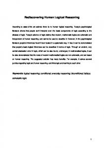
Definition 3.4.5 (Trader). A trader T is a sequence (T1 , T2 , . . .) where each Tn is a trading strategy for day n. We can visualize a trader as a person who gets to see the day n, think for a while, and then produce a trading strategy for day n, which will observe the history of market prices up to and including day n and execute a market order to buy and sell different sentences at the prevailing market prices. We will often consider the set of efficiently computable traders, which have to produce their trading strategy in a time polynomial in n. We can visualize e.c. traders as traders who are computationally limited: each day they get to think for longer and longer—we can imagine them writing computer programs each morning that assist them in their analysis of the market prices—but their total runtime may only grow polynomially in n. If s := Tn [φ] > 0, we say that T buys s shares of φ on day n, and if s < 0, we say that T sells |s| shares of φ on day n. Similarly, if d := Tn [1] > 0, we say that T receives d dollars on day n, and if d < 0, we say that T pays out |d| dollars on day n. Each trade Tn has value zero according to Pn , regardless of what market P it is executed in. Clever traders are the ones who make trades that are later revealed by a deductive process D to have a high worth (e.g., by purchasing shares of provable sentences when the price is low). As an example, a trader T with a basic grasp of arithmetic and skepticism about some of the market P’s confident conjectures might execute the following trade orders on day n: Table 1: Visualizing markets and trades Sentence φ :↔ 1 + 1 = 2
Market prices Pn (φ) = 90¢
Trade Tn [φ] = 4 shares
ψ :↔ 1 + 1 6= 2
Pn (ψ) = 5¢
Tn [ψ] = −3 shares
χ :↔ “Goldbach’s conjecture”
Pn (χ) = 98¢
Tn [χ] = −1 share
The net value of the shares bought and sold at these prices would be 4 · 90¢ − 3 · 5¢ − 1 · 98¢ = $2.47, so if those three sentences were the only sentences bought and sold by Tn , Tn [1] would be −2.47. Trade strategies are a special case of affine combinations of sentences: Definition 3.4.6 (Affine Combination). An F -combination A : S ∪ {1} → Fn is an affine expression of the form A := c + α1 φ1 + · · · + αk φk ,
where (φ1 , . . . , φk ) are sentences and (c, α1 , . . . , αk ) are in F . We define Rcombinations, Q-combinations, and EF -combinations analogously. We write A[1] for the trailing coefficient c, and A[φ] for the coefficient of φ, which is 0 if φ 6∈ (φ1 , . . . , φk ). The rank of A is defined to be the maximum rank among all its coefficients. Given any valuation V, we abuse notation in the usual way and define the value of A (according to V) linearly by: V(A) := c + α1 V(φ1 ) + · · · + αk V(φk ). An F -combination progression is a sequence A of affine combinations where An has rank ≤ n. An EF -combination progression is defined similarly.
Note that a trade T is an F -combination, and the holdings T (P) from T against P is a Q-combination. We will use affine combinations to encode the net holdings P i≤n Ti (P) of a trader after interacting with a market P, and later to encode linear inequalities that hold between the truth values of different sentences. 19
3.5
Exploitation
We will now define exploitation, beginning with an example. Let L be the language of PA, and D be a PA-complete deductive process. Consider a market P that assigns Pn (“1 + 1 = 2”) = 0.5 for all n, and a trader who buys one share of “1 + 1 = 2” each day. Imagine a reasoner behind the market obligated to buy and sell shares at the listed prices, who is also obligated to pay out $1 to holders of φ-shares if and when D says φ. Let t be the first day when “1 + 1 = 2” ∈ Dt . On each day, the reasoner receives 50¢ from T , but after day t, the reasoner must pay $1 every day thereafter. They lose 50¢ each day, and T gains 50¢ each day, despite the fact that T never risked more than $t/2. In cases like these, we say that T exploits P. With this example in mind, we define exploitation as follows: Definition 3.5.1 (Exploitation). A trader T is said to exploit a valuation sequence V relative to a deductive process D if the set of values n �P o �� + V W T n ∈ N , W ∈ PC(D ) i n i≤n
is bounded below, but not bounded above.
P Given a world W, the number W( i≤n Ti (P)) is the value of the trader’s net holdings after interacting with the market PP, where a share of φ is valued at $1 if φ is true in W and $0 otherwise. The set {W( i≤n Ti (P)) | n ∈ N+ , W ∈ PC(Dn )} is the set of all assessments of T ’s net worth, across all time, according to worlds that were propositionally consistent with D at the time. We informally call these plausible assessments of the trader’s net worth. Using this terminology, Definition 3.5.1 says that a trader exploits the market if their plausible net worth is bounded below, but not above. Roughly speaking, we can imagine that there is a person behind the market who acts as a market maker, obligated to buy and sell shares at the listed prices. We can imagine that anyone who sold a φ-share is obligated to pay $1 if and when D says φ. Then, very roughly, a trader exploits the market if they are able to make unbounded returns off of a finite investment. This analogy is illustrative but incomplete—traders can exploit the market even if they never purchase a sentence that appears in D. For example, let φ and ψ be two sentences such that (φ ∨ ψ) is provable in PA, but such that neither φ nor ψ is provable in PA. Consider a trader that bought 10 φ-shares at a price of 20¢ each, and 10 ψ-shares at a price of 30¢ each. Once D says (φ ∨ ψ), all remaining p.c. worlds will agree that the portfolio −5 + 10φ + 10ψ has a value of at least +5, despite the fact that neither φ nor ψ is ever proven. If the trader is allowed to keep buying φ and ψ shares at those prices, they would exploit the market, despite the fact that they never buy decidable sentences. In other words, our notion of exploitation rewards traders for arbitrage, even if they arbitrage between sentences that never “pay out”.
3.6
Main Result
Recall the logical induction criterion: Definition 3.0.1 (The Logical Induction Criterion). A market P is said to satisfy the logical induction criterion relative to a deductive process D if there is no efficiently computable trader T that exploits P relative to D. A market P meeting this criterion is called a logical inductor over D. We may now state our main result:
20
Theorem 3.6.1. For any deductive process D, there exists a computable belief sequence P satisfying the logical induction criterion relative to D. Proof. In Section 5, we show how to take an arbitrary deductive process D and construct a computable belief sequence LIA. Theorem 5.4.2 shows that LIA is a logical inductor relative to the given D. Definition 3.6.2 (Logical Inductor over Γ). Given a theory Γ, a logical inductor over a Γ-complete deductive process D is called a logical inductor over Γ. Corollary 3.6.3. For any recursively axiomatizable theory Γ, there exists a computable belief sequence that is a logical inductor over Γ.
4
Properties of Logical Inductors
Here is an intuitive argument that logical inductors perform good reasoning under logical uncertainty: Consider any polynomial-time method for efficiently identifying patterns in logic. If the market prices don’t learn to reflect that pattern, a clever trader can use that pattern to exploit the market. Thus, a logical inductor must learn to identify those patterns. In this section, we will provide evidence supporting this intuitive argument, by demonstrating a number of desirable properties possessed by logical inductors. The properties that we demonstrate are broken into twelve categories: 1. Convergence and Coherence: In the limit, the prices of a logical inductor describe a belief state which is fully logically consistent, and represents a probability distribution over all consistent worlds. 2. Timely Learning: For any efficiently computable sequence of theorems, a logical inductor learns to assign them high probability in a timely manner, regardless of how difficult they are to prove. (And similarly for assigning low probabilities to refutable statements.) 3. Calibration and Unbiasedness: Logical inductors are well-calibrated and, given good feedback, unbiased. 4. Learning Statistical Patterns: If a sequence of sentences appears pseudorandom to all reasoners with the same runtime as the logical inductor, it learns the appropriate statistical summary (assigning, e.g., 10% probability to the claim “the nth digit of π is a 7” for large n, if digits of π are actually hard to predict). 5. Learning Logical Relationships: Logical inductors inductively learn to respect logical constraints that hold between different types of claims, such as by ensuring that mutually exclusive sentences have probabilities summing to at most 1. 6. Non-Dogmatism: The probability that a logical inductor assigns to an independent sentence φ is bounded away from 0 and 1 in the limit, by an amount dependent on the complexity of φ. In fact, logical inductors strictly dominate the universal semimeasure in the limit. This means that we can condition logical inductors on independent sentences, and when we do, they perform empirical induction. 7. Conditionals: Given a logical inductor P, the market given by the conditional probabilities P(− | ψ) is a logical inductor over D extended to include ψ. Thus, when we condition logical inductors on new axioms, they continue to perform logical induction. 21
8. Expectations: Logical inductors give rise to a well-behaved notion of the expected value of a logically uncertain variable. 9. Trust in Consistency: If the theory Γ underlying a logical inductor’s deductive process is expressive enough to talk about itself, then the logical inductor learns inductively to trust Γ. 10. Reasoning about Halting: If there’s an efficient method for generating programs that halt, a logical inductor will learn in a timely manner that those programs halt (often long before having the resources to evaluate them). If there’s an efficient method for generating programs that don’t halt, a logical inductor will at least learn not to expect them to halt for a very long time. 11. Introspection: Logical inductors “know what they know”, in that their beliefs about their current probabilities and expectations are accurate. 12. Self-Trust: Logical inductors trust their future beliefs. For the sake of brevity, proofs are deferred to Section 6 and the appendix. Some example proofs are sketched in this section, by outlining discontinuous traders that would exploit any market that lacked the desired property. The deferred proofs define polynomial-time continuous traders that approximate those discontinuous strategies. In what follows, let L be a language of propositional logic; let S be the set of sentences written in L; let Γ ⊂ S be a computably enumerable set of propositional formulas written in L (such as PA, where the propositional variables are prime sentences in first-order logic, as discussed in Section 2); and let P be a computable logical inductor over Γ, i.e., a market satisfying the logical induction criterion relative to some Γ-complete deductive process D. We assume in this section that Γ is consistent. Note that while the computable belief sequence LIA that we define has finite support on each day, in this section we assume only that P is a market. We do this because our results below hold in this more general case, and can be applied to LIA as a special case. In sections 4.8-4.12 we will assume that Γ can represent computable functions. This assumption is not necessary until Section 4.8.
4.1
Convergence and Coherence
Firstly, the market prices of a logical inductor converge: Theorem 4.1.1 (Convergence). The limit P∞ : S → [0, 1] defined by P∞ (φ) := lim Pn (φ) n→∞
exists for all φ. Proof sketch.
(Proof in: 6.1 or B.4.)
Roughly speaking, if P never makes up its mind about φ, then it can be exploited by a trader arbitraging shares of φ across different days. More precisely, suppose by way of contradiction that the limit P∞ (φ) does not exist. Then for some p ∈ [0, 1] and ε > 0, we have Pn (φ) < p − ε infinitely often and also Pn (φ) > p + ε infinitely often. A trader can wait until Pn (φ) < p − ε and then buy a share in φ at the low market price of Pn (φ). Then the trader waits until some later m such that Pm (φ) > p+ε, and sells back the share in φ at the higher price. This trader makes a total profit of 2ε every time Pn (φ) oscillates in this way, at no risk, and therefore exploits P. Since P implements a logical inductor, this is not possible; therefore the limit P∞ (φ) must in fact exist.
22
This sketch showcases the main intuition for the convergence of P, but elides a number of crucial details. In particular, the trader we have sketched makes use of discontinuous trading functions, and so is not a well-formed trader. These details are treated in Section 6.1. Next, the limiting beliefs of a logical inductor represent a coherent probability distribution: Theorem 4.1.2 (Limit Coherence). P∞ is coherent, i.e., it gives rise to an internally consistent probability measure Pr on the set PC(Γ) of all worlds consistent with Γ, defined by the formula Pr(W(φ) = 1) := P∞ (φ). In particular, if Γ contains the axioms of first-order logic, then P∞ defines a probability measure on the set of first-order completions of Γ. Proof sketch.
(Proof in: 6.2 or C.10.)
The limit P∞ (φ) exists by the convergence theorem, so Pr is welldefined. Gaifman (1964) shows that Pr defines a probability measure over PC(D∞ ) so long as the following three implications hold for all sentences φ an ψ: • If Γ ⊢ φ, then P∞ (φ) = 1,
• If Γ ⊢ ¬φ, then P∞ (φ) = 0, • If Γ ⊢ ¬(φ ∧ ψ), then P∞ (φ ∨ ψ) = P∞ (φ) + P∞ (ψ).
Let us demonstrate each of these three properties. First suppose that Γ ⊢ φ, but P∞ (φ) = 1−ε for some ε > 0. Then shares of φ will be underpriced, as they are worth 1 in every consistent world, but only cost 1 − ε. There is a trader who waits until φ is propositionally provable from Dn , and until Pn (φ) has approximately converged, and then starts buying shares of φ every day at the price Pn (φ). Since φ has appeared in D, the shares immediately have a minimum plausible value of $1. Thus the trader makes 1 − Pn (φ) ≈ ε profit every day, earning an unbounded total value, contradicting the logical induction criterion. But P cannot be exploited, so P∞ (φ) must be 1. Similarly, if Γ ⊢ ¬φ but P∞ (φ) = ε > 0, then a trader could exploit P by selling off shares in φ for a profit of Pn (φ) ≈ ε each day. Finally, suppose that Γ ⊢ ¬(φ ∧ ψ), but for some ε > 0, P∞ (φ ∨ ψ) = P∞ (φ) + P∞ (ψ) ± ε. Then there is a trader that waits until Pn has approximately converged on these sentences, and until ¬(φ ∧ ψ) is propositionally provable from Dn . At that point it’s a good deal to sell (buy) a share in φ ∨ ψ, and buy (sell) a share in each of φ and ψ; the stocks will have values that cancel out in every plausible world. Thus this trader makes a profit of ≈ ε from the price differential, and can then repeat the process. Thus, they would exploit P. But this is impossible, so P∞ must be coherent. Theorem 4.1.2 says that if P were allowed to run forever, and we interpreted its prices as probabilities, then we would find its beliefs to be perfectly consistent. In the limit, P assigns probability 1 to every theorem and 0 to every contradiction. On independent sentences, its beliefs obey the constraints of probability theory; if φ provably implies ψ, then the probability of ψ converges to a point no lower than the limiting probability of φ, regardless of whether they are decidable. The resulting probabilities correspond to a probability distribution over all possible ways that Γ could be completed. 23
This justifies interpreting the market prices of a logical inductor as probabilities. Logical inductors are not the first computable procedure for assigning probabilities to sentences in a manner that is coherent in the limit; the algorithm of Demski (2012) also has this property. The main appeal of logical induction is that their beliefs become reasonable in a timely manner, outpacing the underlying deductive process.
4.2
Timely Learning
It is not too difficult to define a reasoner that assigns probability 1 to all (and only) the provable sentences, in the limit: simply assign probability 0 to all sentences, and then enumerate all logical proofs, and assign probability 1 to the proven sentences. The real trick is to recognize patterns in a timely manner, well before the sentences can be proven by slow deduction. Logical inductors learn to outpace deduction on any efficiently computable sequence of provable statements.3 To illustrate, consider our canonical example where Dn is the set of all theorems of PA provable in at most n characters, and suppose φ is an e.c. sequence of theorems which are easy to generate but difficult to prove. Let f (n) be the length of the shortest proof of φn , and assume that f is some fast-growing function. At any given time n, the statement φn is ever further out beyond Dn —it might take 1 day to prove φ1 , 10 days to prove φ2 , 100 days to prove φ3 , and so on. One might therefore expect that φn will also be “out of reach” for Pn , and that we have to wait until a much later day close to f (n) before expecting Pf (n) (φn ) to be accurate. However, this is not the case! After some finite time N , P will recognize the pattern and begin assigning high probability to φ in a timely manner. Theorem 4.2.1 (Provability Induction). Let φ be an e.c. sequence of theorems. Then Pn (φn ) hn 1. Furthermore, let ψ be an e.c. sequence of disprovable sentences. Then Pn (ψn ) hn 0. Proof sketch.
(Proof in: 6.5 or C.3.)
Consider a trader that acts as follows. First wait until the time a when Pa (φa ) drops below 1 − ε and buy a share of φa . Then wait until φa is worth 1 in all worlds plausible at time f (a). Then repeat this process. If Pn (φn ) drops below 1 − ε infinitely often, then this trader makes ε profit infinitely often, off of an initial investment of $1, and therefore exploits the market. P is inexploitable, so Pn (φn ) must converge to 1. By a similar argument, Pn (ψn ) must converge to 0.4 In other words, P will learn to start believing φn by day n at the latest, despite the fact that φn won’t be deductively confirmed until day f (n), which is potentially much later. In colloquial terms, if φ is a sequence of facts that can be generated efficiently, then P inductively learns the pattern, and its belief in φ becomes accurate faster than D can computationally verify the individual sentences. For example, imagine that prg(n) is a program with fast-growing runtime, which always outputs either 0, 1, or 2 for all n, but such that there is no proof of this in the general case. Then “∀x : prg(x) = 0 ∨ prg(x) = 1 ∨ prg(x) = 2” 3. Recall that a sequence x is efficiently computable iff there exists a computable function n 7→ xn with runtime polynomial in n. 4. The traders sketched here are optimized for ease of proof, not for efficiency—a clever trader trying to profit from low prices on efficiently computable theorems would be able to exploit the market faster than this.
24
is not provable. Now consider the sequence of statements � prg012 := “prg(n) = 0 ∨ prg(n) = 1 ∨ prg(n) = 2” n∈N+
where each prg012n states that prg outputs a 0, 1, or 2 on that n in particular. Each individual prg012n is provable (it can be proven by running prg on input n), and prg012 is efficiently computable (because the sentences themselves can be written down quickly, even if prg is very difficult to evaluate). Thus, provability induction says that any logical inductor will “learn the pattern” and start assigning high probabilities to each individual prg012n no later than day n. Imagine that D won’t determine the output of prg(n) until the f (n)th day, by evaluating prg(n) in full. Provability induction says that P will eventually recognize the pattern prg012 and start assigning high probability to prg012n no later than the nth day, f (n) − n days before the evaluation finishes. This is true regardless of the size of f (n), so if f is fast-growing, P will outpace D by an ever-growing margin. Analogy: Ramanujan and Hardy. Imagine that the statements φ are being output by an algorithm that uses heuristics to generate mathematical facts without proofs, playing a role similar to the famously brilliant, often-unrigorous mathematician Srinivasa Ramanujan. Then P plays the historical role of the beliefs of the rigorous G.H. Hardy who tries to verify those results according to a slow deductive process (D). After Hardy (P) verifies enough of Ramanujan’s claims (φ≤n ), he begins to trust Ramanujan, even if the proofs of Ramanujan’s later conjectures are incredibly long, putting them ever-further beyond Hardy’s current abilities to rigorously verify them. In this story, Hardy’s inductive reasoning (and Ramanujan’s also) outpaces his deductive reasoning. This idiom of assigning the right probabilities to φn no later than day n will be common throughout the paper, so we give it a name. Definition 4.2.2 (Timely Manner). Let φ be an e.c. sequence of sentences, and p be an e.c. sequence of rational numbers. We say that P assigns p to φ in a timely manner if for every ε > 0, there exists a time N such that for all n > N , |Pn (φn ) − pn | < ε. In other words, P assigns p to φ in a timely manner if Pn (φn ) hn pn . Note that there are no requirements on how large N gets as a function of ε. As such, when we say that P assigns probabilities p to φ in a timely manner, it may take a very long time for convergence to occur. (See Section 5.5 for a discussion.) As an example, imagine the reasoner who recognizes that sentences of the form “1 + 1 + · · · + 1 is even” are true iff the number of ones is even. Let φ be the sequence where φn is the version of that sentence with 2n ones. If the reasoner starts writing a probability near 100% in the φn cell by day n at the latest, then intuitively, she has begun incorporating the pattern into her beliefs, and we say that she is assigning high probabilities to φ in a timely manner. We can visualize ourselves as taking P’s belief states, sorting them by φ on one axis and days on another, and then looking at the main diagonal of cells, to check the probability of each φn on day n. Checking the nth sentence on the nth day is a rather arbitrary choice, and we might hope that a good reasoner would assign high probabilities to e.c. sequences of theorems at a faster rate than that. It is easy to show that this is the case, by the closure properties of efficient computability. For example, if φ is an e.c. sequence of theorems, then so are φ2n and φ2n+1 , which each enumerate half of φ at twice the speed, so by Theorem 4.2.1 (Provability Induction), P will eventually learn to believe φ at a rate of at least two per day. Similarly, P 25
will learn to believe φ3n and φn2 and φ10n3 +3 in a timely manner, and so on. Thus, up to polynomial transformations, it doesn’t really matter which diagonal we check when checking whether a logical inductor has begun “noticing a pattern”. Furthermore, we will show that if P assigns the correct probability on the main diagonal, then P also learns to keep them there: Theorem 4.2.3 (Persistence of Knowledge). Let φ be an e.c. sequence of sentences, and p be an e.c. sequence of rational-number probabilities. If P∞ (φn ) hn pn , then sup |Pm (φn ) − pn | hn 0.
m≥n
Furthermore, if P∞ (φn ) .n pn , then sup Pm (φn ) .n pn , m≥n
and if P∞ (φn ) &n pn , then inf Pm (φn ) &n pn .
m≥n
(Proof in: B.6.)
In other words, if P assigns p to φ in the limit, then P learns to assign probability near pn to φn at all times m ≥ n. This theorem paired with the closure properties of the set of efficiently computable sequences means that checking the probability of φn on the nth day is a fine way to check whether P has begun recognizing a pattern encoded by φ. As such, we invite the reader to be on the lookout for statements of the form Pn (φn ) as signs that P is recognizing a pattern, often in a way that outpaces the underlying deductive process. Theorems 4.2.1 (Provability Induction) and 4.2.3 (Persistence of Knowledge) only apply when the pattern of limiting probabilities is itself efficiently computable. For example, consider the sequence of sentences � πAeq7 := “π[Ack(n, n)] = 7” n∈N+
where π[i] is the ith digit in the decimal expansion of π and Ack is the Ackermann function. Each individual sentence is decidable, so the limiting probabilities are 0 for some πAeq7n and 1 for others. But that pattern of 1s and 0s is not efficiently computable (assuming there is no efficient way to predict the Ackermann digits of π), so provability induction has nothing to say on the topic. In cases where the pattern of limiting probabilities are not e.c., we can still show that if P is going to make its probabilities follow a certain pattern eventually, then it learns to make its probabilities follow that pattern in a timely manner. For instance, assume that each individual sentence πAeq7n (for n > 4) is going to spend a long time sitting at 10% probability before eventually being resolved to either 1 or 0. Then P will learn to assign Pn (πAeq7n ) ≈ 0.1 in a timely manner:
Theorem 4.2.4 (Preemptive Learning). Let φ be an e.c. sequence of sentences. Then lim inf Pn (φn ) = lim inf sup Pm (φn ). n→∞
n→∞ m≥n
Furthermore, lim sup Pn (φn ) = lim sup inf Pm (φn ). n→∞
n→∞ m≥n
(Proof in: B.3.)
Let’s unpack Theorem 4.2.4. The quantity supm≥n Pm (φn ) is an upper bound on the price Pm (φn ) on or after day n, which we can interpret as the highest price tag that that P will ever put on φn after we first start checking it on n. We can imagine a sequence of these values: On day n, we start watching φn . As time goes on, its price travels up and down until eventually settling somewhere. This happens 26
for each n. The limit infimum of supm≥n Pm (φn ) is the greatest lower bound p past which a generic φn (for n large) will definitely be pushed after we started watching it. Preemptive Learning says that if P always eventually pushes φn up to a probability at least p, then it will learn to assign each φn a probability at least p in a timely manner (and similarly for least upper bounds). For example, if each individual πAeq7n is eventually recognized as a claim about digits of π and placed at probability 10% for a long time before being resolved, then P learns to assign it probability 10% on the main diagonal. In general, if P is going to learn a pattern eventually, it learns it in a timely manner. This leaves open the question of whether a logical inductor P is smart enough to recognize that the πAeq7 should each have probability 10% before they are settled (assuming the Ackermann digits of π are hard to predict). We will return to that question in Section 4.4, but first, we examine the reverse question.
4.3
Calibration and Unbiasedness
Theorem 4.2.1 (Provability Induction) shows that logical inductors are good at detecting patterns in what is provable. Next, we ask: when a logical inductor learns a pattern, when must that pattern be real? In common parlance, a source of probabilistic estimates is called well calibrated if among statements where it assigns a probability near p, the estimates are correct with frequency roughly p. In the case of reasoning under logical uncertainty, measuring calibration is not easy. Consider the sequence clusters constructed from correlated clusters of size 1, 10, 100, 1000, . . . , where the truth value of each cluster is determined by the parity of a late digit of π: clusters1 clusters2 :↔ · · · :↔ clusters11 clusters12 :↔ · · · :↔ clusters111 clusters112 :↔ · · · :↔ clusters1111
:↔“π[Ack(1, 1)] :↔“π[Ack(2, 2)] :↔“π[Ack(3, 3)] :↔“π[Ack(4, 4)]
is is is is
even” even” even” even”
and so on. A reasoner who can’t predict the parity of the Ackermann digits of π should assign 50% (marginal) probability to any individual clustersn for n large. But consider what happens if the 9th cluster turns out to be true, and the next billion sentences are all true. A reasoner who assigned 50% to those billion sentences was assigning the right probabilities, but their calibration is abysmal: on the billionth day, they have assigned 50% probability a billion sentences that were overwhelmingly true. And if the 12th cluster comes up false, then on the trillionth day, they have assigned 50% probability to a trillion sentences that were overwhelmingly false! In cases like these, the frequency of truth oscillates eternally, and the good reasoner only appears well-calibrated on the rare days where it crosses 50%. The natural way to correct for correlations such as these is to check P’s conditional probabilities instead of its marginal probabilities. This doesn’t work very well in our setting, because given a logical sentence φ, the quantity that we care about will almost always be the marginal probability of φ. The reason we deal with sequences is because that lets us show that φ has reasonable probabilities relative to various related sentences. For example, if φ := “prg(32) = 17”, then we can use our theorems to relate the probability of φ to the probability of the sequence (“prg(n) = 17”)n∈N+ , and to the sequence (“prg(32) = n”)n∈N+ , and to the sequence (“prg(n) > n”)n∈N+ , and so on, to show that φ eventually has reasonable beliefs about prg (hopefully before P has the resources to simply evaluate prg on input 32). But at the end of the day, we’ll want to reason about the marginal probability of φ itself. In this case, approximately-well-calibrated conditional probabilities wouldn’t buy us much: there are 2n−1 possible truth assignments to the first n − 1 elements of φ, so if we try to compute the marginal probability of φn from all the different conditional probabilities, exponentially many small errors would render the answer useless. Furthermore, intuitively, if φ is utterly unpredictable to P, then the probabilities of all the different truth assignments to φ≤n−1 will go to 27
0 as n gets large, which means the conditional probabilities won’t necessarily be reasonable. (In Section 4.4 will formalize a notion of pseudorandomness.) Despite these difficulties, we can recover some good calibration properties on the marginal probabilities if we either (a) restrict our consideration to sequences where the average frequency of truth converges; or (b) look at subsequences of φ where P has “good feedback” about the truth values of previous elements of the subsequence, in a manner defined below. To state our first calibration property, we will define two different sorts of indicator functions that will prove useful in many different contexts. Definition 4.3.1 (Theorem Indicator). Given a sentence φ, define ThmΓ (φ) to be 1 if Γ ⊢ φ and 0 otherwise. Definition 4.3.2 (Continuous Threshold Indicator). Let δ > 0 be a rational number, and x and y be real numbers. We then define 0 if x ≤ y x−y Indδ (x > y) := if y y) has no false positives, and that it is linear in the region between y and y + δ. We define Indδ (x < y) analogously, and we define Indδ (a < x < b) := min(Indδ (x > a), Indδ (x < b)). Observe that we can generalize this definition to the case where x and y are expressible features, in which case Indδ (x > y) is an expressible [0, 1]-feature. Now we can state our calibration theorem. Theorem 4.3.3 (Recurring Calibration). Let φ be an e.c. sequence of decidable sentences, a and b be rational P numbers, δ be an e.c. �sequence of positive rational numbers, and suppose that n Indδi (a < Pi (φi ) < b) i∈N+ = ∞. Then, if the sequence ! P i≤n Indδi (a < Pi (φi ) < b) · ThmΓ (φi ) P i≤n Indδi (a < Pi (φi ) < b) + n∈N
converges, it converges to a point in [a, b]. Furthermore, if it diverges, it has a limit point in [a, b]. (Proof in: D.3.)
Roughly, this says that if Pn (φn ) ≈ 80% infinitely often, then if we look at the subsequence where it’s 80%, the limiting frequency of truth on that subsequence is 80% (if it converges). In colloquial terms, on subsequences where P says 80% and it makes sense to talk about the frequency of truth, the frequency of truth is 80%, i.e., P isn’t seeing shadows. If the frequency of truth diverges—as in the case with clusters—then P is still well-calibrated infinitely often, but its calibration might still appear abysmal at times (if they can’t predict the swings). Note that calibration alone is not a very strong property: a reasoner can always cheat to improve their calibration (i.e., by assigning probability 80% to things that they’re sure are true, in order to bring up the average truth of their “80%” predictions). What we really want is some notion of “unbiasedness”, which says that there is no efficient method for detecting a predictable bias in a logical inductor’s beliefs. This is something we can get on sequences where the limiting frequency of truth converges, though again, if the limiting frequency of truth diverges, all we can guarantee is a limit point. +
Definition 4.3.4 (Divergent Weighting). A divergentPweighting w ∈ [0, 1]N is an infinite sequence of real numbers in [0, 1], such that n wn = ∞. 28
Note that divergent weightings have codomain [0, 1] as opposed to {0, 1}, meaning the weightings may single out fuzzy subsets of the sequence. For purposes of intuition, imagine that w is a sequence of 0s and 1s, in which case each w can be interpreted as a subsequence. The constraint that the wn sum to ∞ ensures that this subsequence is infinite. Definition 4.3.5 (Generable From P). A sequence of rational numbers q is called generable from P if there exists an e.c. EF-progression q † such that qn† (P) = qn for all n. In this case we say that q is P-generable. P-generable R-sequences, Q-combination sequences, and R-combination sequences are defined analogously. Divergent weightings generable from P are fuzzy subsequences that are allowed to depend continuously (via expressible market features) on the market history. For example, the sequence (Ind0.01 (Pn (φn ) > 0.5))n∈N+ is a P-generable sequence that singles out all times n when Pn (φn ) is greater than 50%. Note that the set of P-generable divergent weightings is larger than the set of e.c. divergent weightings, as the P-generable weightings are allowed to vary continuously with the market prices. Theorem 4.3.6 (Recurring Unbiasedness). Given an e.c. sequence of decidable sentences φ and a P-generable divergent weighting w, the sequence P i≤n wi · (Pi (φi ) − ThmΓ (φi )) P i≤n wi
has 0 as a limit point. In particular, if it converges, it converges to 0.
(Proof in: D.2.)
Letting w = (1, 1, . . .), this theorem says that the difference between the average probability Pn (φn ) and the average frequency of truth is 0 infinitely often (and 0 always, if the latter converges). Letting each wn be Indδ (a < Pn (φn ) < b), we recover Theorem 4.3.3 (Recurring Calibration). In general, the fraction in Theorem 4.3.6 can be interpreted as a measure of the “bias” of P on the fuzzy subsequence of φ singled out by w. Then this theorem says that P is unbiased on all P-generable subsequences where the frequency of truth converges (and unbiased infinitely often on subsequences where it diverges). Thus, if an e.c. sequence of sentences can be decomposed (by any P-generable weighting) into subsequences where the frequency of truth converges, then P learns to assign probabilities such that there is no efficient method for detecting a predictable bias in its beliefs. However, not every sequence can be broken down into well-behaved subsequences by a P-generable divergent weighting (if, for example, the truth values move “pseudorandomly” in correlated clusters, as in the case of clusters). In these cases, it is natural to wonder whether there are any conditions where P will be unbiased anyway. Below, we show that the bias converges to zero whenever the weighting w is sparse enough that P can gather sufficient feedback about φn in between guesses: Definition 4.3.7 (Deferral Function). A function f : N+ → N+ is called a deferral function if 1. f (n) > n for all n, and 2. f (n) can be computed in time polynomial in f (n), i.e., if there is some algorithm and a polynomial function h such that for all n, the algorithm computes f (n) within h(f (n)) steps. If f is a deferral function, we say that f defers n to f (n). Theorem 4.3.8 (Unbiasedness From Feedback). Let φ be any e.c. sequence of decidable sentences, and w be any P-generable divergent weighting. If there exists a 29
strictly increasing deferral function f such that the support of w is contained in the image of f and ThmΓ (φf (n) ) is computable in O(f (n + 1)) time, then P i≤n wi · (Pi (φi ) − ThmΓ (φi )) P hn 0. i≤n wi In this case, we say “w allows good feedback on φ”.
(Proof in: D.5.)
In other words, P is unbiased on any subsequence of the data where a polynomialtime machine can figure out how the previous elements of the subsequence turned out before P is forced to predict the next one. This is perhaps the best we can hope for: On ill-behaved sequences such as clusters, where the frequency of truth diverges and (most likely) no polynomial-time algorithm can predict the jumps, the Pn (φn ) might be pure guesswork. So how well does P perform on sequences like clusters? To answer, we turn to the question of how P behaves in the face of sequences that it finds utterly unpredictable.
4.4
Learning Statistical Patterns
Consider the digits in the decimal expansion of π. A good reasoner thinking about the 101,000,000 th digit of π, in lieu of any efficient method for predicting the digit before they must make their prediction, should assign roughly 10% probability to that digit being a 7. We will now show that logical inductors learn statistical patterns of this form. To formalize this claim, we need some way of formalizing the idea that a sequence is “apparently random” to a reasoner. Intuitively, this notion must be defined relative to a specific reasoner’s computational limitations. After all, the digits of π are perfectly deterministic; they only appear random to a reasoner who lacks the resources to compute them. Roughly speaking, we will define a sequence to be pseudorandom (relative to P) if there is no e.c. way to single out any one subsequence that is more likely true than any other subsequence, not even using expressions written in terms of the market prices (by way of expressible features): Definition 4.4.1 (Pseudorandom Sequence). Given a set S of divergent weightings (Definition 4.3.4), a sequence φ of decidable sentences is called pseudorandom with frequency p over S if, for all weightings w ∈ S, P i≤n wi · ThmΓ (φi ) P lim n→∞ i≤n wi exists and is equal to p.
Note that if the sequence φ is actually randomly generated (say, by adding (c1 , c2 , . . .) to the language of Γ, and tossing a coin weighted with probability p towards heads for each i, to determine whether to add ci or ¬ci as an axiom) then φ is pseudorandom with frequency p almost surely.5 Now: Theorem 4.4.2 (Learning Pseudorandom Frequencies). Let φ be an e.c. sequence of decidable sentences. If φ is pseudorandom with frequency p over the set of all P-generable divergent weightings, then Pn (φn ) hn p. (Proof in: 6.4 or D.8.) 5. Note that actually adding randomness to Γ in this fashion is not allowed, because we assumed that the axioms of Γ are recursively enumerable. It is possible to construct a logical inductor that has access to a source of randomness, by adding one bit of randomness to the market each day, but that topic is beyond the scope of this paper.
30
For example, consider again the sequence πAeq7 where the nth element says that the Ack(n, n)th decimal digit of π is a 7. The individual πAeq7n statements are easy to write down (i.e., efficiently computable), but each one is difficult to decide. Assuming there’s no good way to predict the Ackermann digits of π using a P-generable divergent weighting, P will assign probability 10% to each πAeq7n in a timely manner, while it waits for the resources to determine whether the sentence is true or false. Of course, on each individual πAeq7n , P’s probability will go to 0 or 1 eventually, i.e., limm→∞ Pm (πAeq7n ) ∈ {0, 1}. Theorem 4.4.2 still tells us nothing about how P handles clusters (defined above), because the frequency of truth in that sequence diverges, so it does not count as pseudorandom by the above definition. To handle this case we will weaken our notion of pseudorandomness, so that it includes more sequences, yielding a stronger theorem. We will do this by allowing sequences to count as pseudorandom so long as the limiting frequency of truth converges on “independent subsequences” where the n + 1st element of the subsequence doesn’t come until after the nth element can be decided, as described below. Refer to Garrabrant, Soares, and Taylor (2016) for a discussion of why this is a good way to broaden the set of sequences that count as pseudorandom. Definition 4.4.3 (f -Patient Divergent Weighting). Let f be a deferral function. We say that a divergent weighting w is f -patient if there is some constant C such that, for all n, f (n) X wi (P) ≤ C i=n
In other words, w is f -patient if the weight it places between days n and f (n) is bounded.
While we are at it, we will also strengthen Theorem 4.4.2 in three additional ways: we will allow the probabilities on the sentences to vary with time, and with the market prices, and we will generalize hn to &n and .n . Definition 4.4.4 (Varied Pseudorandom Sequence). Given a deferral function f , a set S of f -patient divergent weightings, an e.c. sequence φ of Γ-decidable sentences, and a P-generable sequence p of rational probabilities, φ is called a p-varied pseudorandom sequence (relative to S) if, for all w ∈ S, P i≤n wi · (pi − ThmΓ (φi )) P hn 0. i≤n wi Furthermore, we can replace hn with &n or .n , in which case we say φ is varied pseudorandom above p or varied pseudorandom below p, respectively.
Theorem 4.4.5 (Learning Varied Pseudorandom Frequencies). Given an e.c. sequence φ of Γ-decidable sentences and a P-generable sequence p of rational probabilities, if there exists some f such that φ is p-varied pseudorandom (relative to all f -patient P-generable divergent weightings), then Pn (φn ) hn pn . Furthermore, if φ is varied pseudorandom above or below p, then the hn may be replaced with &n or .n (respectively). (Proof in: D.7.) Thus we see that P does learn to assign marginal probabilities Pn (clustersn ) ≈ 0.5, assuming the Ackermann digits of π are actually difficult to predict. Note that while Theorem 4.4.5 requires each pn to be rational, the fact that the theorem is generalized to varied pseudorandom above/below sequences means that Theorem 4.4.5 is a strict generalization of Theorem 4.4.2 (Learning Pseudorandom Frequencies). In short, Theorem 4.4.5 shows that logical inductors reliably learn in a timely manner to recognize appropriate statistical patterns, whenever those patterns (which may vary over time and with the market prices) are the best available method for predicting the sequence using P-generable methods. 31
4.5
Learning Logical Relationships
Most of the above properties discuss the ability of a logical inductor to recognize patterns in a single sequence—for example, they recognize e.c. sequences of theorems in a timely manner, and they fall back on the appropriate statistical summaries in the face of pseudorandomness. We will now examine the ability of logical inductors to learn relationships between sequences. Let us return to the example of the computer program prg which outputs either 0, 1, or 2 on all inputs, but for which this cannot be proven in general by Γ. Theorem 4.2.1 (Provability Induction) says that the pattern � prg012 := “prg(n) = 0 ∨ prg(n) = 1 ∨ prg(n) = 2” n∈N+
will be learned, in the sense that P will assign each prg012n a probability near 1 in a timely manner. But what about the following three individual sequences? � prg0 := “prg(n) = 0” n∈N+ � prg1 := “prg(n) = 1” n∈N+ � prg2 := “prg(n) = 2” n∈N+
None of the three sequences is a sequence of only theorems, so provability induction does not have much to say. If they are utterly pseudorandom relative to r, then Theorem 4.4.5 (Learning Varied Pseudorandom Frequencies) says that P will fall back on the appropriate statistical summary, but that tells us little in cases where there are predictable non-conclusive patterns (e.g., if prg(i) is more likely to output 2 when helper(i) outputs 17). In fact, if P is doing good reasoning, the probabilities on the (prg0n , prg1n , prg2n ) triplet ought to shift, as P gains new knowledge about related facts and updates its beliefs. How could we tell if those intermediate beliefs were reasonable? One way is to check their sum. If P believes that prg(i) ∈ {0, 1, 2} and it knows how disjunction works, then it should be the case that whenever Pn (prg012t ) ≈ 1, Pn (prg0t ) + Pn (prg1t ) + Pn (prg2t ) ≈ 1. And this is precisely the case. In fact, logical inductors recognize mutual exclusion between efficiently computable tuples of any size, in a timely manner:
Theorem 4.5.1 (Learning Exclusive-Exhaustive Relationships). Let φ1 , . . . , φk be k e.c. sequences of sentences, such that for all n, Γ proves that φ1n , . . . , φkn are exclusive and exhaustive (i.e. exactly one of them is true). Then Pn (φ1n ) + · · · + Pn (φkn ) hn 1. Proof sketch.
(Proof in: C.11.)
Consider the trader that acts as follows. On day n, they check the prices of φ1n . . . φkn . If the sum of the prices is higher (lower) than 1 by some fixed threshold ε > 0, they sell (buy) a share of each, wait until the values of the shares are the same in every plausible world, and make a profit of ε. (It is guaranteed that eventually, in every plausible world exactly one of the shares will be valued at 1.) If the sum goes above 1+ε (below 1 − ε) on the main diagonal infinitely often, this trader exploits P. Logical inductors are inexploitable, so it must be the case that the sum of the prices goes to 1 along the main diagonal. This theorem suggests that logical inductors are good at learning to assign probabilities that respect logical relationships between related sentences. To show that this is true in full generality, we will generalize Theorem 4.5.1 to any linear inequalities that hold between the actual truth-values of different sentences. First, we define the following convention:
32
Convention 4.5.2 (Constraint). An R-combination A can be viewed as a constraint, in which case we say that a valuation V satisfies the constraint if V(A) ≥ 0. For example, the constraint AND := −2 + φ + ψ says that both φ and ψ are true, and it is satisfied by W iff W(φ) = W(ψ) = 1. As another example, the pair of constraints XOR := (1 − φ − ψ, φ + ψ − 1) say that exactly one of φ and ψ is true, and are satisfied by P7 iff P7 (φ) + P7 (ψ) = 1. Definition 4.5.3 (Bounded Combination Sequence). By BCS(P) (mnemonic: bounded combination sequences) we denote the set of all P-generable Rcombination sequences A that are bounded, in the sense that there exists some bound b such that kAn k1 ≤ b for all n, where k−k1 includes the trailing coefficient. Theorem 4.5.4 (Affine Provability Induction). Let A ∈ BCS(P) and b ∈ R. If, for all consistent worlds W ∈ PC(Γ) and all n ∈ N+ , it is the case that W(An ) ≥ b, then Pn (An ) &n b, and similarly for = and hn , and for ≤ and .n .
(Proof in: C.2.)
For example, consider the constraint sequence A := 1 − prg0n − prg1n − prg2n
�
n∈N+
For all n and all consistent worlds W ∈ PC(Γ), the value W(An ) is 0, so applying Theorem 4.5.5 to A, we get that Pn (An ) hn 0. By linearity, this means Pn (prg0n ) + Pn (prg1n ) + Pn (prg2n ) hn 1, i.e., P learns that the three sequences are mutually exclusive and exhaustive in a timely manner, regardless of how difficult prg is to evaluate. Affine Provability Induction is a generalization of this idea, where the coefficients may vary (day by day, and with the market prices). We can push this idea further, as follows: Theorem 4.5.5 (Affine Coherence). Let A ∈ BCS(P). Then lim inf
inf
n→∞ W∈PC(Γ)
W(An ) ≤ lim inf P∞ (An ) ≤ lim inf Pn (An ), n→∞
n→∞
and lim sup Pn (An ) ≤ lim sup P∞ (An ) ≤ lim sup n→∞
n→∞
sup
W(An ).
n→∞ W∈PC(Γ)
(Proof in: C.1.)
This theorem ties the ground truth on A, to the value of A in the limit, to the value of A on the main diagonal. In words, it says that if all consistent worlds value An in (a, b) for n large, then P∞ values An in (c, d) ⊆ (a, b) for n large (because P∞ is a weighted mixture of all consistent worlds), and P learns to assign probabilities such that Pn (An ) ∈ (c, d) in a timely manner. In colloquial terms, P learns in a timely manner to respect all linear inequalities that actually hold between sentences, so long as those relationships can be enumerated in polynomial time. For example, if helper(i)=err always implies prg(i)=0, P will learn this pattern, and start assigning probabilities to Pn (“prg(n)=0”) which are no lower than 33
those of Pn (“helper(n)=err”). In general, if a series of sentences obey some complicated linear inequalities, then so long as those constraints can be written down in polynomial time, P will learn the pattern, and start assigning probabilities that respect those constraints in a timely manner. This doesn’t mean that P will assign the correct values (0 or 1) to each sentence in a timely manner; that would be impossible for a deductively limited reasoner. Rather, P’s probabilities will start satisfying the constraints in a timely manner. For example, imagine a set of complex constraints holds between seven sequences, such that exactly three sentences in each septuplet are true, but it’s difficult to tell which three. Then P will learn this pattern, and start ensuring that its probabilities on each septuplet sum to 3, even if it can’t yet assign particularly high probabilities to the correct three. If we watch an individual septuplet as P reasons, other constraints will push the probabilities on those seven sentences up and down. One sentence might be refuted and have its probability go to zero. Another might get a boost when P discovers that it’s likely implied by a high-probability sentence. Another might take a hit when P discovers it likely implies a low-probability sentence. Throughout all this, Theorem 4.5.5 says that P will ensure that the seven probabilities always sum to ≈ 3. P’s beliefs on any given day arise from this interplay of many constraints, inductively learned. Observe that Affine Coherence is a direct generalization of Theorem 4.2.1 (Provability Induction). One way to interpret this theorem is that it says that P is very good at learning inductively to predict long-running computations. Given any e.c. sequence of statements about the computation, if they are true then P learns to believe them in a timely manner, and if they are false then P learns to disbelieve them in a timely manner, and if they are related by logical constraints (such as by exclusivity or implication) to some other e.c. sequence of statements, then P learns to make its probabilities respect those constraints in a timely manner. This is one of the main reasons why we think this class of algorithms deserves the name of “logical inductor”. Affine Coherence can also be interpreted as an approximate coherence condition on the finite belief-states of P. It says that if a certain relationship among truth values is going to hold in the future, then P learns to make that relationship hold approximately in its probabilities, in a timely manner.6 In fact, we can use this idea to strengthen every theorem in sections 4.2-4.4, as below. (Readers without interest in the strengthened theorems are invited to skip to Section 4.6.) Affine Strengthenings Observe that Theorem 4.5.4 (Affine Provability Induction) is a strengthening of Theorem 4.2.1 (Provability Induction). Theorem 4.5.6 (Persistence of Affine Knowledge). Let A ∈ BCS(P). Then lim inf inf Pm (An ) = lim inf P∞ (An ) n→∞ m≥n
n→∞
and lim sup sup Pm (An ) = lim sup P∞ (An ). n→∞ m≥n
n→∞
(Proof in: B.5.) 6. Another notion of approximate coherence goes by the name of “inductive coherence” (Garrabrant, Fallenstein, et al. 2016). A reasoner is called inductively coherent if (1) Pn (⊥) hn 0; (2) Pn (φn ) converges whenever φ is efficiently computable and each φn provably implies φn+1 ; and (3) for all efficiently computable sequences of provably mutually exclusive and exhaustive triplets (φn , ψn , χn ), Pn (φn )+Pn (ψn )+Pn (χn ) hn 1. Garrabrant, Fallenstein, et al. show that inductive coherence implies coherence in the limit, and argue that this is a good notion of approximate coherence. Theorems 4.1.2 (Limit Coherence) and 4.5.5 (Affine Coherence) imply inductive coherence, and indeed, logical induction is a much stronger notion.
34
To see that this is a generalization of Theorem 4.2.3 (Persistence of Knowledge), it might help to first replace A with a sequence p of rational probabilities. Theorem 4.5.7 (Affine Preemptive Learning). Let A ∈ BCS(P). Then lim inf Pn (An ) = lim inf sup Pm (An ) n→∞
n→∞ m≥n
and lim sup Pn (An ) = lim sup inf Pm (An ) . n→∞
n→∞ m≥n
(Proof in: B.2.)
Definition 4.5.8 (Determined via Γ). We say that a R-combination A is determined via Γ if, in all worlds W ∈ PC(Γ), the value W(A) is equal. Let ValΓ (A) denote this value. Similarly, a sequence A of R-combinations is said to be determined via Γ if An is determined via Γ for all n. Theorem 4.5.9 (Affine Recurring Unbiasedness). If A ∈ BCS(P) is determined via Γ, and w is a P-generable divergent weighting, P i≤n wi · (Pi (Ai ) − ValΓ (Ai )) P i≤n wi has 0 as a limit point. In particular, if it converges, it converges to 0.
(Proof
in: D.1.)
Theorem 4.5.10 (Affine Unbiasedness from Feedback). Given A ∈ BCS(P) that is determined via Γ, a strictly increasing deferral function f such that ValΓ (An ) can be computed in time O(f (n + 1)), and a P-generable divergent weighting w such that the support of w is contained in the image of f , P i≤n wi · (Pi (Ai ) − ValΓ (Ai )) P hn 0. i≤n wi In this case, we say “w allows good feedback on A”.
(Proof in: D.4.)
Theorem 4.5.11 (Learning Pseudorandom Affine Sequences). Given a A ∈ BCS(P) which is determined via Γ, if there exists deferral function f such that for any P-generable f -patient divergent weighting w, P i≤n wi · ValΓ (Ai ) P &n 0, i≤n wi
then
Pn (An ) &n 0, and similarly for hn , and .n .
4.6
(Proof in: D.6.)
Non-Dogmatism
Cromwell’s rule says that a reasoner should not assign extreme probabilities (0 or 1) except when applied to statements that are logically true or false. The rule was named by Lindley (1991), in light of the fact that Bayes’ theorem says that a Bayesian reasoner can never update away from probabilities 0 or 1, and in reference to the famous plea:
35
I beseech you, in the bowels of Christ, think it possible that you may be mistaken. – Oliver Cromwell The obvious generalization of Cromwell’s rule to a setting where a reasoner is uncertain about logic is that they also should not assign extreme probabilities to sentences that have not yet been proven or disproven. Logical inductors do not satisfy this rule, as evidenced by the following theorem: Theorem 4.6.1 (Closure under Finite Perturbations). Let P and P′ be markets with Pn = P′n for all but finitely many n. Then P is a logical inductor if and only if P′ is a logical inductor. (Proof in: G.7.) This means that we can take a logical inductor, completely ruin its beliefs on the 23rd day (e.g., by setting P23 (φ) = 0 for all φ), and it will still be a logical inductor. Nevertheless, there is still a sense in which logical inductors are non-dogmatic, and can “think it possible that they may be mistaken”: Theorem 4.6.2 (Non-Dogmatism). If Γ 0 φ then P∞ (φ) < 1, and if Γ 0 ¬φ then P∞ (φ) > 0. Proof sketch.
(Proof in: G.4.)
Consider a trader that watches φ and buys whenever it gets low, as follows. The trader starts with $1. They spend their first 50 cents when Pn (φ) < 1/2, purchasing one share. They spend their next 25 cents when Pn (φ) < 1/4, purchasing another share. They keep waiting for Pn (φ) to drop low enough that they can spend the next half of their initial wealth to buy one more share. Because φ is independent, there always remains at least one world W such that W(φ) = 1, so if Pn (φ) → 0 as n → ∞ then their maximum plausible profits are $1 + $1 + $1 +. . . which diverges, and they exploit the market. Thus, P∞ (φ) must be bounded away from zero. In other words, if φ is independent from Γ, then P’s beliefs about φ won’t get stuck converging to 0 or 1. By Theorem 4.6.1 (Closure under Finite Perturbations), P may occasionally jump to unwarranted conclusions—believing with “100% certainty”, say, that Euclid’s fifth postulate follows from the first four—but it always corrects these errors, and eventually develops conservative beliefs about independent sentences. Theorem 4.6.2 guarantees that P will be reasonable about independent sentences, but it doesn’t guarantee reasonable beliefs about theories, because theories can require infinitely many axioms. For example, let Γ be a theory of pure first-order logic, and imagine that the language L has a free binary relation symbol “ ∈ ”. Now consider the sequence ZFCaxioms of first-order axioms of Zermelo-Fraenkel set theory (ZFC) which say to interpret “ ∈ ” in the set-theoretic way, and note that ZFCaxioms is infinite. Each individual sentence ZFCaxiomsn is consistent with first-order logic, but if P∞ ’s odds on each axiom were 50:50 and independent, then it would say that the probability of them all being true simultaneously was zero. Fortunately, for any computably enumerable sequence of sentences that are mutually consistent, P∞ assigns positive probability to them all being simultaneously true. Theorem 4.6.3 (Uniform Non-Dogmatism). For any computably enumerable sequence of sentences φ such that Γ ∪ φ is consistent, there is a constant ε > 0 such that for all n, P∞ (φn ) ≥ ε. (Proof in: G.2.)
If φn is the conjunction of the first n axioms of ZFC, Theorem 4.6.3 shows that P∞ assigns positive probability to theories in which the symbol “ ∈ ” satisfies all axioms of ZFC (assuming ZFC is consistent). 36
Reasoning about individual sentences again, we can put bounds on how far each sentence φ is bounded away from 0 and 1, in terms of the prefix complexity κ(φ) of φ, i.e., the length of the shortest prefix that causes a fixed universal Turing machine to output φ.7 Theorem 4.6.4 (Occam Bounds). There exists a fixed positive constant C such that for any sentence φ with prefix complexity κ(φ), if Γ 0 ¬φ, then P∞ (φ) ≥ C2−κ(φ) , and if Γ 0 φ, then P∞ (φ) ≤ 1 − C2−κ(φ) . (Proof in: G.3.)
This means that if we add a sequence of constant symbols (c1 , c2 , . . .) not mentioned in Γ to the language L, then P’s beliefs about statements involving those constants will depend on the complexity of the claim. Roughly speaking, if you ask after the probability of a claim like “c1 = 10 ∧ c2 = 7 ∧ . . . ∧ cn = −3” then the answer will be no lower than the probability that a simplicity prior assigns to the shortest program that outputs (10, 7, . . . , −3). In fact, the probability may be a fair bit higher, if the claim is part of a particularly simple sequence of sentences. In other words, logical inductors can be used to reason about empirical uncertainty as well as logical uncertainty, by using P∞ as a full-fledged sequence predictor: Theorem 4.6.5 (Domination of the Universal Semimeasure). Let (b1 , b2 , . . .) be a sequence of zero-arity predicate symbols in L not mentioned in Γ, and let σ≤n = (σ1 , . . . , σn ) be any finite bitstring. Define P∞ (σ≤n ) := P∞ (“(b1 ↔ σ1 = 1) ∧ (b2 ↔ σ2 = 1) ∧ . . . ∧ (bn ↔ σn = 1)”), such that, for example, P∞ (01101) = P∞ (“¬b1 ∧ b2 ∧ b3 ∧ ¬b4 ∧ b5 ”). Let M be a universal continuous semimeasure. Then there is some positive constant C such that for any finite bitstring σ≤n , P∞ (σ≤n ) ≥ C · M (σ≤n ). (Proof in: G.5.)
In other words, logical inductors can be viewed as a computable approximation to a normalized probability distribution that dominates the universal semimeasure. In fact, this dominance is strict: Theorem 4.6.6 (Strict Domination of the Universal Semimeasure). The universal continuous semimeasure does not dominate P∞ ; that is, for any positive constant C there is some finite bitstring σ≤n such that P∞ (σ≤n ) > C · M (σ≤n ). (Proof in: G.6.)
In particular, by Theorem 4.6.3 (Uniform Non-Dogmatism), logical inductors assign positive probability to the set of all completions of theories like PA and ZFC, 7. We use prefix complexity (the length of the shortest prefix that causes a UTM to output φ) instead of Kolmogorov complexity (the length of the shortest complete program that causes a UTM to output φ) because it makes the proof slightly easier. (And, in the opinion of the authors, prefix complexity is the more natural concept.) Both types of complexity are defined relative to an arbitrary choice of universal Turing machine (UTM), but our theorems hold for every logical inductor regardless of the choice of UTM, because changing the UTM only amounts to changing the constant terms by some fixed amount.
37
whereas universal semimeasures do not. This is why we can’t construct approximately coherent beliefs about logic by fixing an enumeration of logical sentences and conditioning a universal semimeasure on more axioms of Peano arithmetic each day: the probabilities that the semimeasure assigns to those conjunctions must go to zero, so the conditional probabilities may misbehave. (If this were not the case, it would be possible to sample a complete extension of Peano arithmetic with positive probability, because universal semimeasures are approximable from below; but this is impossible. See the proof of Theorem 4.6.6 for details.) While P∞ is limitcomputable, it is not approximable from below, so it can and does outperform the universal semimeasure when reasoning about arithmetical claims.
4.7
Conditionals
One way to interpret Theorem 4.6.5 (Domination of the Universal Semimeasure) is that when we condition P∞ on independent sentences about which it knows nothing, it performs empirical (scientific) induction. We will now show that when we condition P, it also performs logical induction. In probability theory, it is common to discuss conditional probabilities such as Pr(A | B) := Pr(A ∧ B)/Pr(B) (for any B with Pr(B) > 0), where Pr(A | B) is interpreted as the probability of A restricted to worlds where B is true. In the domain of logical uncertainty, we can define conditional probabilities in the analogous way: Definition 4.7.1 (Conditional Probability). Let φ and ψ be sentences, and let V be a valuation with V(ψ) > 0. Then we define � V(φ ∧ ψ)/V(ψ) if V(φ ∧ ψ) < V(ψ) V(φ | ψ) := 1 otherwise. Given a valuation sequence V, we define V(− | ψ) := (V1 (− | ψ), V2 (− | ψ), . . .). Defining V(φ | ψ) to be 1 if V(ψ) = 0 is nonstandard, but convenient for our theorem statements and proofs. The reader is welcome to ignore the conditional probabilities in cases where V(ψ) = 0, or to justify our definition from the principle of explosion (which says that from a contradiction, anything follows). This definition also caps V(φ | ψ) at 1, which is necessary because there’s no guarantee that V knows that φ ∧ ψ should have a lower probability than ψ. For example, if it takes P more than 17 days to learn how “∧” interacts with φ and ψ, then it might be the case that P17 (φ ∧ ψ) = 0.12 and P17 (ψ) = 0.01, in which case the uncapped “conditional probability” of φ ∧ ψ given ψ according to P17 would be twelve hundred percent. This fact doesn’t exactly induce confidence in P(− | ψ). Nevertheless, we have the following theorem: Theorem 4.7.2 (Closure Under Conditioning). The sequence P(− | ψ) is a logical inductor over Γ ∪ {ψ}. Furthermore, given any efficiently computable sequence ψ of sentences, the sequence (P1 (− | ψ1 ), P2 (− | ψ1 ∧ ψ2 ), P3 (− | ψ1 ∧ ψ2 ∧ ψ3 ), . . .) , where the nth pricing is conditioned on the first n sentences in ψ, is a logical inductor over Γ ∪ {ψi | i ∈ N+ }. (Proof in: G.8.) In other words, if we condition logical inductors on logical sentences, the result is still a logical inductor, and so the conditional probabilities of a logical inductor continues to satisfy all the desirable properties satisfied by all logical inductors. This also means that one can obtain a logical inductor for Peano arithmetic by starting with a logical inductor over an empty theory, and conditioning it on PA. With that idea in mind, we will now begin examining questions about logical inductors that assume Γ can represent computable functions, such as questions about P’s beliefs about Γ, computer programs, and itself. 38
4.8
Expectations
In probability theory, it is common to ask the expected (average) value of a variable that takes on different values in different possible worlds. Emboldened by our success with conditional probabilities, we will now define a notion of the expected values of logical variables, and show that these are also fairly well-behaved. This machinery will be useful later when we ask logical inductors for their beliefs about themselves. We begin by defining a notion of logically uncertain variables, which play a role analogous to the role of random variables in probability theory. For the sake of brevity, we will restrict our attention to logically uncertain variables with their value in [0, 1]; it is easy enough to extend this notion to a notion of arbitrary bounded realvalued logically uncertain variables. (It does, however, require carrying a variable’s bounds around everywhere, which makes the notation cumbersome.) To define logically uncertain variables, we will need to assume that Γ is capable of representing rational numbers and proving things about them. Later, we will use expected values to construct sentences that talk about things like the expected outputs of a computer program. Thus, in this section and in the remainder of Section 4, we will assume that Γ can represent computable functions. Definition 4.8.1 (Logically Uncertain Variable). A logically uncertain variable, abbreviated LUV, is any formula X free in one variable that defines a unique value via Γ, in the sense that Γ ⊢ ∃x : (X(x) ∧ ∀x′ : X(x′ ) → x′ = x). We refer to that value as the value of X. If Γ proves that the value of X is in [0, 1], we call X a [0, 1]-LUV. Given a [0, 1]-LUV X and a consistent world W ∈ PC(Γ), the value of X in W is defined to be W(X) := sup {x ∈ [0, 1] | W(“X ≥ x”) = 1} . In other words, W(X) is the supremum of values that do not exceed X according to W. (This rather roundabout definition is necessary in cases where W assigns X a non-standard value.) We write U for the set of all [0, 1]-LUVs. When manipulating logically uncertain variables, we use shorthand like “X < 0.5” for “∀x : X(x) → x < 0.5”. See Section 2 for details. As an example, Half := “ν = 0.5” is a LUV, where the unique real number that makes Half true is rather obvious. A more complicated LUV is TwinPrime := “1 if the twin prime conjecture is true, 0 otherwise”; this is a deterministic quantity (assuming Γ actually proves the twin prime conjecture one way or the other), but it’s reasonable for a limited reasoner to be uncertain about the value of that quantity. In general, if f : N+ → [0, 1] is a computable function then “f (7)” is a LUV, because “f (7)” is shorthand for the formula “γf (7, ν)”, where γf is the predicate of Γ representing f . With LUVs in hand, we can define a notion of P’s expected value for a LUV X on day n with precision k. The obvious idea is to take the sum lim
k→∞
k−1 X i=0
i Pn (“i/k < X ≤ (i + 1)/k”). k
However, if Pn hasn’t yet figured out that X pins down a unique value, then it might put high probability on X being in multiple different intervals, and the simple integral of a [0, 1]-valued LUV could fall outside the [0, 1] interval. This is a nuisance when we want to treat the expectations of [0, 1]-LUVs as other [0, 1]-LUVs, 39
so instead, we will define expectations using an analog of a cumulative distribution function. In probability theory, the expectation of a [0, 1]-valued random variable R1 V with density function ρV is given by E(V ) = 0 x · ρV (x)dx. We can rewrite this using integration by parts as Z 1 Pr(V > x)dx. E(V ) = 0
This motivates the following definition of expectations for LUVs: Definition 4.8.2 (Expectation). For a given valuation V, we define the approximate expectation operator EV k for V with precision k by EV k (X) :=
k−1 X i=0
1 V(“X > i/k”). k
where X is a [0, 1]-LUV. This has the desirable property that EV k (X) ∈ [0, 1], because V(−) ∈ [0, 1]. We will often want to take a limit of EPkn (X) as both k and n approach ∞. We hereby make the fairly arbitrary choice to focus on the case k = n for simplicity, adopting the shorthand En := EPnn . In other words, when we examine how a logical inductor’s expectations change on a sequence of sentences over time, we will (arbitrarily) consider approximate expectations that gain in precision at a rate of one unit per day. We will now show that the expectation operator En possesses properties that make it worthy of that name. Theorem 4.8.3 (Expectations Converge). The limit E∞ : S → [0, 1] defined by E∞ (X) := lim En (X) n→∞
exists for all X ∈ U.
(Proof in: E.4.)
Note that E∞ (X) might not be rational. Because P∞ defines a probability measure over PC(Γ), E∞ (X) is the average value of W(X) across all consistent worlds (weighted by P∞ ). In other words, every LUV X can be seen as a random variable with respect to the measure P∞ , and E∞ acts as the standard expectation operator on P∞ . Furthermore, Theorem 4.8.4 (Linearity of Expectation). Let a, b be bounded P-generable sequences of rational numbers, and let X, Y , and Z be e.c. sequences of [0, 1]-LUVs. If we have Γ ⊢ Zn = an Xn + bn Yn for all n, then an En (Xn ) + bn En (Yn ) hn En (Zn ). (Proof in: E.9.)
For our next result, we want a LUV which can be proven to take value 1 if φ is true and 0 otherwise. Definition 4.8.5 (Indicator LUV). For any sentence φ, we define its indicator LUV by the formula 1(φ) := “(φ ∧ (ν = 1)) ∨ (¬φ ∧ (ν = 0))”. Observe that 1(φ)(1) is equivalent to φ, and 1(φ)(0) is equivalent to ¬φ.
40
Theorem 4.8.6 (Expectations of Indicators). Let φ be an e.c. sequence of sentences. Then En (1(φn )) hn Pn (φn ). (Proof in: E.10.)
In colloquial terms, Theorem 4.8.6 says that a logical inductor learns that asking for the expected value of 1(φ) is the same as asking for the probability of φ. To further demonstrate that expectations work as expected, we will show that they satisfy generalized versions of all theorems proven in sections 4.2-4.5. (Readers without interest in the versions of those theorems for expectations are invited to skip to Section 4.9.) Collected Theorems for Expectations Definition 4.8.7 (LUV Valuation). A LUV valuation is any function U : U → V + [0, 1]. Note that EV n and E∞ are LUV valuations for any valuation V and n ∈ N , and that every world W ∈ PC(Γ) is a LUV valuation. Definition 4.8.8 (LUV Combination). An F -LUV-combination B : U ∪ {1} → Fn is an affine expression of the form B := c + α1 X1 + · · · + αk Xk , where (X1 , . . . , Xk ) are [0, 1]-LUVs and (c, α1 , . . . , αk ) are in F . An EF -LUVcombination, an R-LUV-combination, and a Q-LUV-combination are defined similarly. The following concepts are all defined analogously to how they are defined for sentence combinations: B[1], B[X], rank(B), U(B) for any LUV valuation U, F LUV-combination progressions, EF -LUV-combination progressions, and P-generable LUV-combination sequences. (See definitions 3.4.6 and 4.3.5 for details.) Definition 4.8.9 (Bounded LUV-Combination Sequence). By BLCS(P) (mnemonic: bounded LUV-combination sequences) we denote the set of all P-generable R-LUV-combination sequences B that are bounded, in the sense that there exists some bound b such that kBn k1 ≤ b for all n, where k−k1 includes the trailing coefficient. Theorem 4.8.10 (Expectation Provability Induction). Let B ∈ BLCS(P) and b ∈ R. If, for all consistent worlds W ∈ PC(Γ) and all n ∈ N+ , it is the case that W(Bn ) ≥ b, then En (Bn ) &n b, and similarly for = and hn , and for ≤ and .n . (Proof in: E.8.) Theorem 4.8.11 (Expectation Coherence). Let B ∈ BLCS(P). Then lim inf
inf
n→∞ W∈PC(Γ)
W(Bn ) ≤ lim inf E∞ (Bn ) ≤ lim inf En (Bn ), n→∞
n→∞
and lim sup En (Bn ) ≤ lim sup E∞ (Bn ) ≤ lim sup n→∞
n→∞
sup
W(Bn ).
n→∞ W∈PC(Γ)
(Proof in: E.7.)
Theorem 4.8.12 (Persistence of Expectation Knowledge). Let B ∈ BLCS(P). Then lim inf inf Em (Bn ) = lim inf E∞ (Bn ) n→∞ m≥n
n→∞
and lim sup sup Em (Bn ) = lim sup E∞ (Bn ). n→∞ m≥n
n→∞
(Proof in: E.6.)
41
Theorem 4.8.13 (Expectation Preemptive Learning). Let B ∈ BLCS(P). Then lim inf En (Bn ) = lim inf sup Em (Bn ) n→∞
n→∞ m≥n
and lim sup En (Bn ) = lim sup inf Em (Bn ) . n→∞
n→∞ m≥n
(Proof in: E.3.)
Definition 4.8.14 (Determined via Γ (for LUV-Combinations)). We say that a RLUV-combination B is determined via Γ if, in all worlds W ∈ PC(Γ), the value W(B) is equal. Let ValΓ (B) denote this value. Similarly, a sequence B of R-LUV-combinations is said to be determined via Γ if Bn is determined via Γ for all n. Theorem 4.8.15 (Expectation Recurring Unbiasedness). If B ∈ BLCS(P) is determined via Γ, and w is a P-generable divergent weighting weighting such that the support of w is contained in the image of f , P i≤n wi · (Ei (Bi ) − ValΓ (Bi )) P i≤n wi has 0 as a limit point. In particular, if it converges, it converges to 0.
Theorem 4.8.16 (Expectation Unbiasedness From Feedback). Given B ∈ BLCS(P) that is determined via Γ, a strictly increasing deferral function f such that ValΓ (An ) can be computed in time O(f (n + 1)), and a P-generable divergent weighting w, P i≤n wi · (Ei (Bi ) − ValΓ (Bi )) P hn 0. i≤n wi In this case, we say “w allows good feedback on B”.
(Proof in: E.12.)
Theorem 4.8.17 (Learning Pseudorandom LUV Sequences). Given a B ∈ BLCS(P) which is determined via Γ, if there exists a deferral function f such that for any P-generable f -patient divergent weighting w, P i≤n wi · ValΓ (Bi ) P &n 0, i≤n wi
then
En (Bn ) &n 0. (Proof in: E.13.)
4.9
Trust in Consistency
The theorems above all support the hypothesis that logical inductors develop reasonable beliefs about logic. One might then wonder what a logical inductor has to say about some of the classic questions in meta-mathematics. For example, what does a logical inductor over PA say about the consistency of Peano arithmetic? Definition 4.9.1 (Consistency Statement). Given a recursively axiomatizable theory Γ′ , define the n-consistency statement of Γ′ to be the formula with one free variable ν such that Con(Γ′ )(ν) := “There is no proof of ⊥ from Γ′ with ν or fewer symbols”, 42
written in L using a Gödel encoding. For instance, Con(PA)(“ Ack(10, 10)”) says that any proof of ⊥ from PA requires at least Ack(10, 10) symbols. We further define “Γ′ is consistent” to be the universal generalization “∀n : there is no proof of ⊥ from Γ′ in n or fewer symbols”, and “Γ′ is inconsistent” for its negation. Theorem 4.9.2 (Belief in Finitistic Consistency). Let f be any computable function. Then Pn (Con(Γ)(“f (n)”)) hn 1. (Proof in: C.4.)
In other words, if Γ is in fact consistent, then P learns to trust it for arbitrary finite amounts of time. For any fast-growing function f you can name, P eventually learns to believe Γ is consistent for proofs of length at most f (n), by day n at the latest. In colloquial terms, if we take a logical inductor over PA and show it a computable function f that, on each input n, tries a new method for finding an inconsistency in PA, then the logical inductor will stare at the function for a while and eventually conclude that it’s not going to succeed (by learning to assign low probability to f (n) proving ⊥ from PA by day n at the latest, regardless of how long f runs). That is to say, a logical inductor over PA learns to trust Peano arithmetic inductively. By the same mechanism, a logical inductor over Γ can learn inductively to trust the consistency of any consistent theory, including consistent theories that are stronger than Γ (in the sense that they can prove Γ consistent): Theorem 4.9.3 (Belief in the Consistency of a Stronger Theory). Let Γ′ be any recursively axiomatizable consistent theory. Then Pn (Con(Γ′ )(“f (n)”)) hn 1. (Proof in: C.5.)
For instance, a logical inductor over PA can learn inductively to trust the consistency of ZFC for finite proofs of arbitrary length (assuming ZFC is in fact consistent). These two theorems alone are unimpressive. Any algorithm that assumes consistency until proven otherwise can satisfy these theorems, and because every inconsistent theory admits a finite proof of inconsistency, those naïve algorithms will disbelieve any inconsistent theory eventually. But those algorithms will still believe inconsistent theories for quite a long time, whereas logical inductors learn to distrust inconsistent theories in a timely manner: Theorem 4.9.4 (Disbelief in Inconsistent Theories). Let Γ′ be an e.c. sequence of recursively axiomatizable inconsistent theories. Then Pn (“Γ′n is inconsistent”) hn 1, so
Pn (“Γ′n is consistent”) hn 0. (Proof in: C.6.)
In other words, logical inductors learn in a timely manner to distrust inconsistent theories that can be efficiently named, even if the shortest proofs of inconsistency are very long. Note that Theorem 4.9.2 (Belief in Finitistic Consistency) does not say P∞ (“Γ is consistent”) is equal to 1, nor even that it’s particularly high. On the contrary, by Theorem 4.6.2 (Non-Dogmatism), the limiting probability on that sentence is bounded away from 43
0 and 1 (because both that sentence and its negation are consistent with Γ). Intuitively, D never reveals evidence against the existence of non-standard numbers, so P remains open to the possibility. This is important for Theorem 4.7.2 (Closure Under Conditioning), which say that logical inductors can safely be conditioned on any sequence of statements that are consistent with Γ, but it also means that P will not give an affirmative answer to the question of whether PA is consistent in full generality. In colloquial terms, if you hand a logical inductor any particular computation, it will tell you that that computation isn’t going to output a proof ⊥ from the axioms of PA, but if you ask whether PA is consistent in general, it will start waxing philosophical about non-standard numbers and independent sentences—not unlike a human philosopher. A reasonable objection here is that Theorem 4.9.2 (Belief in Finitistic Consistency) is not talking about the consistency of the Peano axioms, it’s talking about computations that search for proofs of contradiction from PA. This is precisely correct, and brings us to our next topic.
4.10
Reasoning about Halting
Consider the famous halting problem of Turing (1936). Turing proved that there is no general algorithm for determining whether or not an arbitrary computation halts. Let’s examine what happens when we confront logical inductors with the halting problem. Theorem 4.10.1 (Learning of Halting Patterns). Let m be an e.c. sequence of Turing machines, and x be an e.c. sequence of bitstrings, such that mn halts on input xn for all n. Then Pn (“mn halts on input xn ”) hn 1. (Proof in: C.7.)
Note that the individual Turing machines do not need to have fast runtime. All that is required is that the sequence m be efficiently computable, i.e., it must be possible to write out the source code specifying mn in time polynomial in n. The runtime of an individual mn is immaterial for our purposes. So long as the mn all halt on the corresponding xn , P recognizes the pattern and learns to assign high probability to “mn halts on input xn ” no later than the nth day. Of course, this is not so hard on its own—a function that assigns probability 1 to everything also satisfies this property. The real trick is separating the halting machines from the non-halting ones. This is harder. It is easy enough to show that P learns to recognize e.c. sequences of machines that provably fail to halt: Theorem 4.10.2 (Learning of Provable Non-Halting Patterns). Let q be an e.c. sequence of Turing machines, and y be an e.c. sequence of bitstrings, such that qn provably fails to halt on input yn for all n. Then Pn (“qn halts on input yn ”) hn 0. (Proof in: C.8.)
Of course, it’s not too difficult to disbelieve that the provably-halting machines will halt; what makes the above theorem non-trivial is that P learns in a timely manner to expect that those machines won’t halt. Together, the two theorems above say that if there is any efficient method for generating computer programs that definitively either halt or don’t (according to Γ) then P will learn the pattern. The above two theorems only apply to cases where Γ can prove that the machine either halts or doesn’t. The more interesting case is the one where a Turing machine q fails to halt on input y, but Γ is not strong enough to prove this fact. In this case, P∞ ’s probability of q halting on input y is positive, by Theorem 4.6.2 (Non– Dogmatism). Nevertheless, P still learns to stop expecting that those machines will halt after any reasonable amount of time: 44
Theorem 4.10.3 (Learning not to Anticipate Halting). Let q be an e.c. sequence of Turing machines, and let y be an e.c. sequence of bitstrings, such that qn does not halt on input yn for any n. Let f be any computable function. Then Pn (“qn halts on input yn within f (n) steps”) hn 0. (Proof in: C.9.)
For example, let y be an enumeration of all bitstrings, and let q be the constant sequence (q, q, . . .) where q is a Turing machine that does not halt on any input. If Γ cannot prove this fact, then P will never be able to attain certainty about claims that say q fails to halt, but by Theorem 4.10.3, it still learns to expect that q will run longer than any computable function you can name. In colloquial terms, while P won’t become certain that non-halting machines don’t halt (which is impossible), it will put them in the “don’t hold your breath” category (along with some longrunning machines that do halt, of course). These theorems can be interpreted as justifying the intuitions that many computer scientists have long held towards the halting problem: It is impossible to tell whether or not a Turing machine halts in full generality, but for large classes of well-behaved computer programs (such as e.c. sequences of halting programs and provably non-halting programs) it’s quite possible to develop reasonable and accurate beliefs. The boundary between machines that compute fast-growing functions and machines that never halt is difficult to distinguish, but even in those cases, it’s easy to learn to stop expecting those machines to halt within any reasonable amount of time. (See also the work of Calude and Stay [2008] for other formal results backing up this intuition.) One possible objection here is that the crux of the halting problem (and of the Γ-trust problem) are not about making good predictions, they are about handling diagonalization and paradoxes of self-reference. Gödel’s incompleteness theorem constructs a sentence that says “there is no proof of this sentence from the axioms of PA”, and Turing’s proof of the undecidability of the halting problem constructs a machine which halts iff some other machine thinks it loops. P learning to trust Γ is different altogether from P learning to trust itself. So let us turn to the topic of P’s beliefs about P.
4.11
Introspection
Because we’re assuming Γ can represent computable functions, we can write sentences describing the beliefs of P at different times. What happens when we ask P about sentences that refer to itself? For instance, consider a sentence ψ := “Pn (φ) > 0.7” for some specific n and φ, where P’s beliefs about ψ should depend on what its beliefs about φ are on the nth day. Will P figure this out and get the probabilities right on day n? For any particular φ and n it’s hard to say, because it depends on whether P has learned how ψ relates to P and φ yet. If however we take an e.c. sequence of ψ which all say “φ will have probability greater than 0.7 on day n” with n varying, then we can guarantee that P will learn the pattern, and start having accurate beliefs about its own beliefs: Theorem 4.11.1 (Introspection). Let φ be an e.c. sequence of sentences, and a, b be P-generable sequences of probabilities. Then, for any e.c. sequence of positive rationals δ → 0, there exists a sequence of positive rationals ε → 0 such that for all n: 1. if Pn (φn ) ∈ (an + δn , bn − δn ), then Pn (“an < Pn (φn ) < bn ”) > 1 − εn , 2. if Pn (φn ) ∈ / (an − δn , bn + δn ), then Pn (“an < Pn (φn ) < bn ”) < εn . 45
(Proof in: F.1.)
In other words, for any pattern in P’s beliefs that can be efficiently written down (such as “P’s probabilities on φ are between a and b on these days”), P learns to believe the pattern if it’s true, and to disbelieve it if it’s false (with vanishing error). At a first glance, this sort of self-reflection may seem to make logical inductors vulnerable to paradox. For example, consider the sequence of sentences χ0.5 := (“Pn (χ0.5 n ) < 0.5”)n∈N+ such that χ0.5 n is true iff P assigns it a probability less than 50% on day n. Such a sequence can be defined by Gödel’s diagonal lemma. These sentences are probabilistic versions of the classic “liar sentence”, which has caused quite a ruckus in the setting of formal logic (Grim 1991; McGee 1990; Glanzberg 2001; Gupta and Belnap 1993; Eklund 2002). Because our setting is probabilistic, it’s perhaps most closely related to the “unexpected hanging” paradox—χ0.5 n is true iff P thinks it is unlikely on day n. How do logical inductors handle this sort of paradox? Theorem 4.11.2 (Paradox Resistance). Fix a rational p ∈ (0, 1), and define an e.c. sequence of “paradoxical sentences” χp satisfying � � Γ ⊢ χpn ↔ Pn (χpn ) < p for all n. Then
lim Pn (χpn ) = p.
n→∞
(Proof in: F.2.)
A logical inductor responds to paradoxical sentences χp by assigning probabilities that converge on p. For example, if the sentences say “P will assign me a probability less than 80% on day n”, then Pn (once it has learned the pattern) starts assigning probabilities extremely close to 80%—so close that traders can’t tell if it’s slightly above or slightly below. By Theorem 4.3.6 (Recurring Unbiasedness), the frequency of truth in χp≤n will have a limit point at 0.8 as n → ∞, and by the definition of logical induction, there will be no efficiently expressible method for identifying a bias in the price. Let us spend a bit of time understanding this result. After day n, χ0.8 n is “easy” to get right, at least for someone with enough computing power to compute Pn (χ0.8 n ) to the necessary precision (it will wind up very close to 0.8 for large n). Before day n, we can interpret the probability of χ0.8 n as the price of a share that’s going to pay out $1 if the price on day n is less than 80¢, and $0 otherwise. What’s the value of this share? Insofar as the price on day n is going to be low, the value is high; insofar as the price is going to be high, the value is low. So what actually happens on the nth day? Smart traders buy χ0.8 n if its price is lower than 80¢, and sell it if its price is higher than 80¢. By the continuity constraints on the traders, each one has a price at which they stop buying χ0.8 n , and Theorem 4.11.2 (Paradox Resistance) tells us that the stable price exists extremely close to 80¢. Intuitively, it must be so close that traders can’t tell which way it’s going to go, biased on the low side, so that it looks 80% likely to be below and 20% likely to be above to any efficient inspection. For if the probability seemed more than 80% likely to be below, traders would buy; and if it seemed anymore than 20% likely to be above, traders would sell. To visualize this, imagine that your friend owns a high-precision brain-scanner and can read off your beliefs. Imagine they ask you what probability you assign to the claim “you will assign probability 0.7) for some sequence of rational numbers δ → 0, as per Definition 4.3.2. This value is 1 if P will expect the nth bundle to be worth more than 70¢ on day f (n), and 0 otherwise, and intermediate if the case isn’t quite clear. Then � � � � En “X n · Indδn Ef (n) (X n ) > 0.7 ” can be interpreted as P’s expected value of the bundle on day n, in cases where P is going to think it’s worth at least 70¢ on day f (n). Now assume that Indδn (Ef (n) (Xn )) > 0 and divide it out of both sides, in which case the theorem roughly says Enow (X | Elater (X) > 0.7) h Enow (Elater (X) | Elater (X) > 0.7), which says that P’s expected value of the bundle now, given that it’s going to think the bundle has a value of at least 70¢ later, is equal to whatever it expects to think later, conditioned on thinking later that the bundle is worth at least 70¢. Combining this idea with indicator functions, we get the following theorem: Theorem 4.12.4 (Self-Trust). Let f be a deferral function, φ be an e.c. sequence of sentences, δ be an e.c. sequence of positive rational numbers, and p be a P-generable sequence of rational probabilities. Then � � � � � � � � En “1(φn ) · Indδn Pf (n) (φn ) > pn ” &n pn · En “Indδn Pf (n) (φn ) > pn ” .
(Proof in: F.8.)
Very roughly speaking, if we squint at Theorem 4.12.4, it says something like Enow (φ | Plater (φ) > p) & p, i.e., if we ask P what it would believe about φ now if it learned that it was going to believe φ with probability at least p in the future, then it will answer with a probability that is at least p. As a matter of fact, Theorem 4.12.4 actually says something slightly weaker, which is also more desirable. Let each φn be the self-referential sentence “Pf (n) (φn ) < 0.5” which says that the future Pf (n) will assign probability less than 48
0.5 to φn . Then, conditional on Pf (n) (φn ) ≥ 0.5, Pn should believe that the probability of φn is 0. And indeed, this is what a logical inductor will do: � � Pn “φn ∧ (Pf (n) (φn ) ≥ 0.5)” hn 0,
by Theorem 4.2.3 (Persistence of Knowledge), because each of those conjunctions is disprovable. This is why Theorem 4.12.4 uses continuous indicator functions: With discrete conjunctions, the result would be undesirable (not to mention false). What Theorem 4.12.4 says is that P attains self-trust of the “if in the future I will believe x is very likely, then it must be because x is very likely” variety, while retaining the ability to think it can outperform its future self’s beliefs when its future self confronts paradoxes. In colloquial terms, if we ask “what’s your probability on the paradoxical sentence φn given that your future self believes it with probability exactly 0.5?” then P will answer “very low”, but if we ask “what’s your probability on the paradoxical sentence φn given that your future self believes it with probability extremely close to 0.5?” then P will answer “roughly 0.5.” Still speaking roughly, this means that logical inductors trust their future beliefs to be accurate and only change for good reasons. Theorem 4.12.4 says that if you ask “what’s the probability of φ, given that in the future you’re going to believe it’s more than 95% likely?” then you’ll get an answer that’s no less than 0.95, even if the logical inductor currently thinks that φ is unlikely.
5
Construction
In this section, we show how given any deductive process D, we can construct a computable belief sequence, called LIA, that satisfies the logical induction criterion relative to D. Roughly speaking, LIA works by simulating an economy of traders and using Brouwer’s fixed point theorem to set market prices such that no trader can exploit the market relative to D. We will build LIA from three subroutines called MarketMaker, Budgeter, and TradingFirm. Intuitively, MarketMaker will be an algorithm that sets market prices by anticipating what a single trader is about to do, Budgeter will be an algorithm for altering a trader to stay within a certain budget, and TradingFirm will be an algorithm that uses Budgeter to combine together an infinite sequence of carefully chosen e.c. traders (via a sum calculable in finite time) into a single trader that exploits a given market if any e.c. trader exploits that market. Then, LIA will work by using MarketMaker to make a market not exploitable by TradingFirm and hence not exploitable by any e.c. trader, thereby satisfying the logical induction criterion. To begin, we will need a few basic data types for our subroutines to pass around: Definition 5.0.1 (Belief History). An n-belief history P≤n = (P1 , . . . , Pn ) is a finite list of belief states of length n. Definition 5.0.2 (Strategy History). An n-strategy history T≤n = (T1 , . . . , Tn ) is a finite list of trading strategies of length n, where Ti is an i-strategy. Definition 5.0.3 (Support). For any valuation V we define Support(V) := {φ ∈ S | V(φ) 6= 0}, and for any n-strategy Tn we define Support(Tn ) := {φ ∈ S | Tn [φ] 6≡ 0}. Observe that for any belief state P and any n-strategy Tn , Support(P) and Support(Tn ) are computable from the finite lists representing P and Tn .
49
5.1
Constructing MarketMaker
Here we define the MarketMaker subroutine and establish its key properties. Intuitively, given any trader T as input, on each day n, MarketMaker looks at the trading strategy Tn and the valuations P≤n−1 output by MarketMaker on previous days. It then uses an approximate fixed point (guaranteed to exist by Brouwer’s fixed point theorem) that sets prices Pn for that day such that when the trader’s strategy Tn reacts to the prices, the resulting trade Tn (P≤n ) earns at most a very small positive amount of value in any world. Intuitively, the fixed point finds the trader’s “fair prices”, such that they abstain from betting, except possibly to buy sentences at a price very close to $1 or sell them at a price very close to $0, thereby guaranteeing that very little value can be gained from the trade. Lemma 5.1.1 (Fixed Point Lemma). Let Tn be any n-strategy, and let P≤n−1 be any (n−1)-belief history. There exists a valuation V with Support(V) ⊆ Support(Tn ) such that for all worlds W ∈ W: W (Tn (P≤n−1 , V)) ≤ 0. (5.1.1) Proof. We will use Brouwer’s fixed point theorem to find “prices” V such that Tn only ever buys shares for $1 or sells them for $0, so it cannot make a profit in any world. Intuitively, we do this by making a “price adjustment” mapping called fix that moves prices toward 1 or 0 (respectively) as long as Tn would buy or sell (respectively) any shares at those prices, and finding a fixed point of that mapping. First, we let S ′ = Support(Tn ) and focus on the set V ′ := {V | Support(V) ⊆ S ′ }. Observe that V ′ is equal to the natural inclusion of the finite-dimensional cube ′ [0, 1]S in the space of all valuations V = [0, 1]S . We now define our “price adjustment” function fix : V ′ → V ′ as follows: fix(V)(φ) := max(0, min(1, V(φ) + T (P≤n−1 , V)[φ])). This map has the odd property that it adds prices and trade volumes, but it does the trick. Notice that fix is a function from the compact, convex space V ′ to itself, so if it is continuous, it satisfies the antecedent of Brouwer’s fixed point theorem. Observe that fix is in fact continuous, because trade strategies are continuous. Indeed, we required that trade strategies be continuous for precisely this purpose. Thus, by Brouwer’s fixed point theorem, fix has at least one fixed point Vfix that satisfies, for all sentences φ ∈ S ′ , Vfix (φ) = max(0, min(1, Vfix (φ) + Tn (P≤n−1 , Vfix )[φ])). Fix a world W and observe from this equation that if Tn buys some shares of φ ∈ S ′ at these prices, i.e. if Tn (P≤n−1 , Vfix )[φ] > 0, then Vfix (φ) = 1, and in particular, W(φ)−Vfix (φ) ≤ 0. Similarly, if Tn sells some shares of φ, i.e. if Tn (P≤n , Vfix )[φ] < 0, then Vfix (φ) = 0, so W(φ) − Vfix (φ) ≥ 0. In either case, we have 0 ≥ (W(φ) − Vfix (φ)) · Tn (P≤n−1 , Vfix )[φ] since the two factors always have opposite sign (or at least one factor is 0). Summing over all φ, remembering that Tn (V≤n )[φ] = 0 for φ ∈ / S ′ , gives X 0≥ (W(φ) − Vfix (φ)) · Tn (P≤n−1 , Vfix )[φ] φ∈S
= W(Tn (P≤n , Vfix )) − Vfix (Tn (P≤n−1 , Vfix ))
since the values of the “cash” terms W(Tn (P≤n , Vfix )[1]) and Vfix (Tn (P≤n , Vfix )[1]) are by definition both equal to Tn (P≤n , Vfix )[1] and therefore cancel. But Vfix (Tn (P≤n−1 , Vfix )) = 0 50
by definition of a trading strategy, so for any world W, we have 0 ≥ W(Tn (P≤n−1 , Vfix )). Definition/Proposition 5.1.2 (MarketMaker). There exists a computable function, henceforth named MarketMaker, satisfying the following definition. Given as input any n ∈ N+ , any n-strategy Tn , and any (n − 1)-belief history P≤n−1 , MarketMakern (Tn , P≤n−1 ) returns a belief state P with Support(P) ⊆ Support(Tn ) such that for all worlds W ∈ W: W(Tn (P≤n−1 , P)) ≤ 2−n . (5.1.2) Proof. Essentially, we will find a rational approximation P to the fixed point Vfix in the previous lemma, by brute force search. This requires some care, because the set of all worlds is uncountably infinite. First, given Tn and P≤n−1 , let S ′ := Support(Tn ), V ′ = {V | Support(V) ⊆ S ′ }, and take Vfix ∈ V ′ satisfying (5.1.1). Let W ′ := {W′ | Support(W′ ) ∈ S ′ }, and for any W, define W′ ∈ W ′ by � W(φ) if φ ∈ S ′ , ′ W (φ) := 0 otherwise. Observe that for any W ∈ W, the function V ′ → R given by V 7→ W(Tn (P≤n−1 , V)) = W′ (Tn (P≤n−1 , V)) is a continuous function of V that depends only on W′ . Since the set W ′ is finite, the function V 7→ sup W(Tn (P≤n−1 , V)) = max W′ (Tn (P≤n−1 , V)) ′ ′ W ∈W
W∈W
is the maximum of a finite number of continuous functions, and is therefore continuous. Hence there is some neighborhood in V ′ around Vfix with image in (−∞, 2−n ) ⊂ R. By the density of rational points in V ′ , there is therefore some belief state P ∈ V ′ ∩ QS satisfying (5.1.2), as needed. It remains to show that such a P can in fact be found by brute force search. First, recall that a belief state P is a rational-valued finite-support map from S to [0, 1], and so can be represented by a finite list of pairs (φ, q) with φ ∈ S and q ∈ Q ∩ [0, 1]. Since S and [0, 1] ∩ Q are computably enumerable, so is the set of all belief states. Thus, we can computably “search” though all possible Ps, so we need only establish that given n, Tn , and P≤n−1 we can computably decide whether each P in our search satisfies (5.1.2) until we find one. First note that the finite set Support(Tn ) can be computed by searching the expression specifying Tn for all the sentences φ that occur within it. Moreover, equation (5.1.2) need only be be checked for worlds W′ ∈ W ′ , since any other W returns the same value as its corresponding W′ . Now, for any fixed world W′ ∈ W ′ and candidate P, we can compute each value in the language of expressible features X W′ (Tn (P≤n−1 , P)) = Tn (P≤n−1 , P)[1] + W′ (φ) · Tn (P≤n−1 , P)[φ] φ∈S ′
directly by evaluating the expressible features Tn [φ] on the given belief history (P≤n−1 , P), as φ ∈ S ′ varies. Since W ′ is a finite set, we can do this for all W′ with a finite computation. Thus, checking whether a belief state P satisfies condition (5.1.2) is computably decidable, and a solution to (5.1.2) can therefore be found by enumerating all belief states P and searching through them for the first one that works. 51
Lemma 5.1.3 (MarketMaker Inexploitability). Let T be any trader. The sequence of belief states P defined recursively by Pn := MarketMakern (Tn , P≤n−1 ), with base case P1 = MarketMaker(T1 , ()), is not exploited by T relative to any deductive process D. Proof. By the definition of MarketMaker, we have that for every n, the belief state P = Pn satisfies equation (5.1.2), i.e., for all worlds W ∈ W and all n ∈ N+ : W(Tn (P)) ≤ 2−n . Hence by linearity of W, for all n ∈ N+ we have: �P � X X W T (P) = W(Ti (P)) ≤ 2−i < 1. i i≤n i≤n
i≤n
Therefore, given any deductive process D, n �P � o + sup W i≤n Ti (P) n ∈ N , W ∈ PC(Dn ) ≤ 1 < ∞, so T does not exploit P relative to D.
5.2
Constructing Budgeter
Here we introduce a subroutine for turning a trader with potentially infinite losses into a trader that will never have less than −$b in any world W ∈ PC(Dn ) on any day n, for some bound b, in such a way that does not affect the trader if it wouldn’t have fallen below −$b to begin with. Definition/Proposition 5.2.1 (Budgeter). Given any deductive process D, there exists a computable function, henceforth called BudgeterD , satisfying the following definition. Given inputs n and b ∈ N+ , an n-strategy history T≤n , and an (n − 1)belief history P≤n−1 , BudgeterD returns an n-strategy BudgeterD n (b, T≤n , P≤n−1 ), such that �P � if: W T (P ) ≤ −b for some m < n and W ∈ PC(Dm ), i ≤i i≤m then:
BudgeterD n (b, T≤n , P≤n−1 ) = 0,
else:
BudgeterD n (b, T≤n , P≤n−1 ) =
Tn ·
Proof. Let S ′ = world W, write
inf
W∈PC(Dn )
S
i≤n
max1,
(5.2.1) −1
−W(Tn ) �P � b+W T (P ) i ≤i i≤n−1
.
Support(Ti ), W ′ = {W | Support(W) ⊆ S ′ }, and for any W′ (φ) :=
�
W(φ) 0
if φ ∈ S ′ , otherwise.
Now, observe that we can computably check the “if” statement in the function P definition. This is because W( i≤m Ti (P≤i )) depends only on W′ ∈ W ′ , a finite set. We can check whether W′ ∈ PC(Dm ) in finite time by checking whether any assignment of truth values to the finite set of prime sentences occurring in 52
sentences of Dn yields the assignment W′ on Support(W′ ). The set of sentences Dn is computable given n, because D is computable by definition. It remains to show that the “else” expression can be computed and returns an n-trading strategy. First, the infimum can be computed over W′ ∈ W ′ ∩ PC(Dn ), a finite set, since the values in the inf depend only on W′ , and the inf operator itself can be re-expressed in the language of expressible P features using max and multiplication by (−1). The values W′ (Tn ) and W′ ( i≤n−1 Ti (P≤i )) are finite P sums, and the denominator b + W( i≤n−1 Ti (P≤i )) is a fixed positive rational (so we can safely multiply by its reciprocal). The remaining operations are all singlestep evaluations in the language of expressible valuation features, completing the proof. P Let us reflect on the meaning of these operations. The quantity b+W( i −b, then Bnb (P) = Tn (P);
2. for all b, n ∈ N+ and all W ∈ PC(Dn ), we have �P � b W i≤n Bi (P) ≥ −b; b
3. If T exploits P relative to D, then so does B for some b ∈ N+ . Part 1. Proof. Suppose that for some time step n, for all m ≤ n and all worlds W ∈ PC(Dm ) plausible at time m we have �P � W i≤m Ti (P) > −b,
so by linearity of W(−), we have in particular that �P � � b+W i≤n−1 Ti (P) > −W Tn (P) .
Since n − 1 ≤ n, the LHS is positive, so we have � −W Tn (P) �P �. 1> b+W i≤n−1 Ti (P)
Therefore, by the definition of BudgeterD (and T�i (P) = Ti (P≤i � )), since the “if” P clause doesn’t trigger by the assumption on the W i≤m Ti (P) for m < n, , −W(T (P)) �P n � inf 1 max1, Bnb (P) ≡ Tn (P) · W∈PC(Dn ) b+W T (P) i i≤n−1 = Tn (P≤n ) ·
inf
W∈PC(Dn )
1/1
= Tn (P) as needed. 53
Part 2. Proof. Suppose for a contradiction that for some n and some W ∈ PC(Dn ), �P � b B (P) W < −b. i≤n i
Assume that n is the least such day, and fix some such W ∈ PC(Dn ). By the� minimality of� n it must be that W(Bnb (P)) < 0, or else we would have P b W < −b. Since Bnb (P) is a non-negative multiple of Tn (P), we i≤n−1 Bi (P)
6 0, from the definition of BudgeterD also have W(Tn (P)) < 0. However, since Bnb ≡ we have !! , � � −W′ (Tn (P)) b W Bn = W Tn (P) · inf 1 max 1, P W′ ∈PC(Dn ) b + W′ ( i≤n−1 Ti (P)) , ! � � −W(Tn (P)) ≥ W Tn (P) · 1 max 1, (since W Tn (P) < 0) P b + W( i≤n−1 Ti (P)) P � b + W( i≤n−1 Ti (P)) ≥ W Tn (P) · −W(Tn (P)) � P since −W Tn (P) > 0 and Bnb 6≡ 0 implies b + W( i≤n−1 Ti (P)) > 0. Hence, this � �P = −b − W i≤n Ti (P) . Further, since Bnb 6≡ 0, we have �P � for all j ≤ n − 1 : W T (P) > −b, which by Part 1 implies that i i≤j for all j ≤ n − 1 :
Part 3.
Bjb (P) = Tj (P), therefore � �P b W(Bnb ) ≥ −b − W i≤n−1 Bi (P) , hence � �P b ≥ −b. W B (P) i≤n i
Proof. By definition of exploitation, the set n �P � o + W T (P) n ∈ N , W ∈ PC(D ) i n i≤n
is unbounded above, and is strictly bounded below by some integer b. Then by Part 1, for all n we have Tn (P) = Bnb (P). Thus, n �P � o + b W i≤n Bi (P) n ∈ N , W ∈ PC(Dn ) b
is unbounded above and bounded below, i.e., B exploits P relative to D.
5.3
Constructing TradingFirm
Next we define TradingFirm, which combines an (enumerable) infinite sequence of e.c. traders into a single “supertrader” that exploits a given belief sequence P relative to D if any e.c. trader does. It does this by taking each e.c. trader, budgeting it, and scaling its trades down so that traders later in the sequence carry less weight to begin with. To begin, we will need a computable sequence that includes every e.c. trader at least once. The following trick is standard, but we include it here for completeness: 54
Proposition 5.3.1k(Redundant Enumeration of e.c. Traders). There exists a computable sequence (T )k∈N+ of e.c. traders such that every e.c. trader occurs at least once in the sequence. Proof. Fix a computable enumeration of all ordered pairs (Mk , fk ) where Mk is a Turing machine and fk is a polynomial with coefficients in Z. We define a computable function ECT : {Turing machines} × {Integer polynomials} × (n ∈ N+ ) → {n-strategies} that runs as follows: ECT(M, f, n) first runs M (n) for up to f (n) time steps, and if in that time M (n) halts and returns a valid n-strategy Tn , then ECT(M, f, n) returns that strategy, otherwise it returns 0 (as an n-strategy). Observe that ECT(Mk , fk , −) is always an e.c. trader, and that every e.c. trader occurs as ECT(Mk , fk , −) for some k. Definition/Proposition 5.3.2 (TradingFirm). Given any deductive process D, there exists a computable function, henceforth called TradingFirmD , satisfying the k following definition. By Proposition 5.3.1, we fix a computable enumeration T including every e.c. trader at least once, and let � k Tn if n ≥ k k Sn = 0 otherwise. Given input n ∈ N+ and an (n − 1)-belief history P≤n−1 , TradingFirmD returns an n-strategy given by X X k TradingFirmD 2−k−b · BudgeterD (5.3.2) n (P≤n−1 ) = n (b, S≤n , P≤n−1 ). k∈N+ b∈N+
Proof. We need only show that the infinite sum in equation (5.3.2) is equivalent to a computable finite sum. Writing k Bnb,k = BudgeterD n (b, S≤n , P≤n−1 ),
(an n-strategy), the sum on the RHS of (5.3.2) is equivalent to X X 2−k−b · Bnb,k . k∈N+ b∈N+
Since Snk = 0 for k > n, we also have Bnb,k = 0 for k > n, so the sum is equivalent to X X = 2−k−b · Bnb,k . k≤n b∈N+
P Now, assume Cn is a positive integer such that i≤n kSik (V)k1 < Cn for all k ≤ n and any valuation sequence V (we will show below that such a Cn can be computed from P≤n−1 ).� Since the valuations W and P are always [0, 1]-valued, for any m ≤ n � P P k k the values W i≤m kSi (P≤m )k1 > −Cn . i≤m Si (P≤m ) are bounded below by − By property 1 of BudgeterD (Lemma 5.2.2.1), Bnb,k = Snk when b > Cn , so the sum is equivalent to X X X X = 2−k−b · Snk 2−k−b · Bnb,k + k≤n b>Cn
k≤n b≤Cn
=
X X
k≤n b≤Cn
2−k−b · Bnb,k + 55
X
k≤n
2−k−Cn · Snk
which is a finite sum of trading strategies, and hence is itself a trading strategy. Since the Bnb,k and the Snk are computable from P≤n−1 , this finite sum is computable. It remains to justify our assumption that integers Cn can be computed from P P≤n−1 with Cn > i≤n kSik (V)k1 for all k ≤ n and V. To see this, first consider how to bound a single expressible feature ξ. We can show by induction on the structure of ξ (see A.2) that, given constant bounds on the absolute value |ζ(V)| of each subexpression ζ of ξ, we can compute a constant bound on |ξ(V)|; for example, the bound on ζ ·η is the product of the bound on ζ and the bound on η. Thus, given a single trading strategy Sik and any φ, we can compute a constant upper bound on P |Sik [φ](V)| for all V. Since kSik (V)k1 ≤ φ∈Support(S k ) 2|Sik [φ](V)| and Support(Sik ) i P is computable, we can bound each kSik (V)k1 , and hence also i≤n kSik (V)k1 , as needed. Lemma 5.3.3 (Trading Firm Dominance). Let P be any sequence of belief states, and D be a deductive process. If there exists any e.c. trader T that exploits P relative to D, then the sequence � � TradingFirmD n (P≤n−1 ) n∈N+
also exploits P (relative to D). k
Proof. Suppose that some e.c. trader exploits P. That trader occurs as T for some k in the enumeration used by TradingFirmD . First, we show that S k (from the definition of TradingFirmD ) also exploits P. It suffices to show that there exist constants c1 ∈ R+ and c2 ∈ R such that for all n ∈ N+ and W ∈ PC(Dn ), �P � �P � k k W i≤n Sn (P) ≥ c1 · W i≤n Tn (P) + c2 .
P Taking c1 = 1 and c2 = − i f (φ, ε). Then f must be uncomputable. Proof. Suppose for contradiction that such a computable f were given. We will show that f could be used to computably determine whether Γ ⊢ φ for an arbitrary sentence φ, a task which is known to be impossible for a first-order theory that can represent computable functions. (If we assumed further that Γ were sound as a theory of the natural numbers, this would allow us to solve the halting problem by letting φ be a sentence of the form “M halts”.) Given a sentence φ, we run two searches in parallel. If we find that Γ ⊢ φ, then we return True. If we find that for some b, n ∈ N+ we have � � 1 1 n > f φ, and Pn (φ) ≤ 1 − , (5.5.1) b b then we return False. Both of these conditions are computably enumerable since f , Pn , and verifying witnesses to Γ ⊢ φ are computable functions. Suppose� first that Γ ⊢ φ. Then by definition of f we have Pn (φ) > 1 − 1b for all n > f φ, 1b , and hence we find a witness for Γ ⊢ φ and return True. Now suppose that Γ 0 φ. Then by Theorem 4.6.2 (Non-Dogmatism) we have that P∞ (φ) < 1 − ε for some ε > 0, and hence for some b and all sufficiently large n we have Pn (φ) < 1 − 1/b. Therefore 5.5.1 holds and we return False. Thus our search always halts and returns a Boolean value that correctly indicates whether Γ ⊢ φ.
6
Selected Proofs
In this section, we exhibit a few selected stand-alone proofs of certain key theorems. These theorems hold for any P satisfying the logical induction criterion, which we recall here: Definition 3.0.1 (The Logical Induction Criterion). A market P is said to satisfy the logical induction criterion relative to a deductive process D if there is no efficiently computable trader T that exploits P relative to D. A market P meeting this criterion is called a logical inductor over D. Only our notation (Section 2), framework (Section 3), and continuous threshold indicator (Definition 4.3.2) are needed to understand the results and proofs in this section. Shorter proofs of these theorems can be found in the appendix, but those rely on significantly more machinery.
6.1
Convergence
Recall Theorem 4.1.1 and the proof sketch given: Theorem 4.1.1 (Convergence). The limit P∞ : S → [0, 1] defined by P∞ (φ) := lim Pn (φ) n→∞
exists for all φ. Proof sketch. Roughly speaking, if P never makes up its mind about φ, then it can be exploited by a trader arbitraging shares of φ across different days. More precisely, suppose by way of contradiction that the limit P∞ (φ) does not exist. Then for some p ∈ [0, 1] and ε > 0, we have Pn (φ) < p − ε infinitely often and also Pn (φ) > p + ε infinitely often. A trader can wait until Pn (φ) < p − ε and then buy a share in φ at the low market price of 58
Pn (φ). Then the trader waits until some later m such that Pm (φ) > p+ε, and sells back the share in φ at the higher price. This trader makes a total profit of 2ε every time Pn (φ) oscillates in this way, at no risk, and therefore exploits P. Since P implements a logical inductor, this is not possible; therefore the limit P∞ (φ) must in fact exist. We will define a trader T that executes a strategy similar to this one, and hence exploits the market P if limn→∞ Pn (φ) diverges. To do this, there are two technicalities we must deal with. First, the strategy outlined above uses a discontinuous function of the market prices Pn (φ), and therefore is not permitted. This is relatively easy to fix using the continuous indicator functions of Definition 4.3.2. The second technicality is more subtle. Suppose we define our trader to buy φ-shares whenever their price Pn (φ) is low, and sell them back whenever their price is high. Then it is possible that the trader makes the following trades in sequence against the market P: buy 10 φ-shares on consecutive days, then sell 10 φ-shares; then buy 100 φ-shares consecutively, and then sell them off; then buy 1000 φ-shares, then sell them off; and so on. Although this trader makes profit on each batch, it always spends more on the next batch, taking larger and larger risks (relative to the remaining plausible worlds). Then the plausible value of this trader’s holdings will be unbounded below, and so it does not exploit P. In short, this trader is not tracking its budget, and so may have unboundedly negative plausible net worth. We will fix this problem by having our trader T track how many net φ-shares it has bought, and not buying too many, thereby maintaining bounded risk. This will be sufficient to prove the theorem. Proof of Theorem 4.1.1. Suppose by way of contradiction that the limit P∞ does not exist. Then, for some sentence φ and some rational numbers p ∈ [0, 1] and ε > 0, we have that Pn (φ) < p − ε infinitely often and Pn (φ) > p + ε infinitely often. We will show that P can be exploited by a trader T who buys below and sells above these prices infinitely often, contrary to the logical induction criterion. Definition of the trader T . We will define T recursively along with another sequence of EF-combinations H (mnemonic: “holdings”) which tracks the sum of the trader’s previous trades. Our base cases are T1 := 0 H1 := 0. For n > 1, we define a recurrence whereby T will buy some φ-shares whenever φ∗n < p − ε/2, up to (1 − Hn−1 [φ]) shares when φ∗n < p − ε, and sells some φ-shares whenever φ∗n > p + ε/2, up to Hn−1 shares when φ∗n > p + ε: Tn [φ] := (1 − Hn−1 [φ]) · Indε/2 (φ∗n < p − ε/2)
− Hn−1 [φ] · Indε/2 (φ∗n > p + ε/2),
Tn := Tn [φ] · (φ − φ∗n ) Hn := Hn−1 + Tn .
(6.1.1)
The trade coefficients T [φ] are chosen so that the number of φ-shares Hn [φ] that it owns is always in [0, 1] (it never buys more than 1 − Hn−1 [φ] and never sells more than Hn−1 [φ]). Observe that each Tn is a valid trading strategy for day n (see Definition 3.4.4) because it is of the form ξ · (φ − φ∗n ). To complete the definition, we must ague that T is efficiently computable. For this, observe that the 3n + 2 definition (:=) equations defining T1 , . . . , Tn above can be written down in time polynomial in n. Thus, a combination of feature expressions defining Tn from scratch can be written down in poly(n) time (indeed, the expression is just a concatenation of n copies of the three “:=” equations written above, along with the base cases), so T is efficiently computable.
59
Proof of exploitation. To show T exploits P over D, we must compute P upper and lower bounds on the set of plausible values W(Hn (P)) (since Hn = i≤n Tn ) for worlds W ∈ PC(Dn ). While proving exploitation, we leave the constant argument P implicit to reduce clutter, writing, e.g., φ∗i for φ∗i (P) = Pi (φ), Tn [φ] for Tn [φ](P), and so on. First, since each Ti [1] = −T [φ] · φ∗i , the trader’s “cash” held on day n is X X Hn [1] = Ti [1] = − Ti [φ] · φ∗i i≤n
i≤n
which we can regroup, to compare the prices φ∗i to p, as X X � Hn [1] = Ti [φ] · (p − φ∗i ) − p · Ti [φ] i≤n
=
X i≤n
i≤n
∗i
� Ti [φ] · (p − φ ) − p · Hn [φ].
Now, if φ∗i < p − ε/2 then Ti [φ] ≥ 0, if φ∗i > p + ε/2 then Ti [φ] ≤ 0, and if p − ε/2 ≤ φ∗i ≤ p + ε/2 then Ti [φ] = 0, so for all i the product Ti [φ] · (p − φ∗i ) is equal to or greater than |Ti [φ]| · ε/2: X Hn [1] ≥ −p · Hn [φ] + |Ti [φ]| · ε/2. i≤n
Moreover, by design, Hn [φ] ∈ [0, 1] for all n, so X Hn [1] ≥ −p + |Ti [φ]| · ε/2. i≤n
Now, by assumption, φ∗i lies above and below (p − ε, p + ε) infinitely often, so from P equation (6.1.1), Hi [φ] = 0 and Hi [φ] = 1 infinitely often. Since the sum i≤n |Ti [φ]| is the total variation in the sequence Hi [φ], it must diverge (by the triangle inequality) as n → ∞, so lim Hn [1] = ∞.
n→∞
Moreover, in any world W, the trader’s non-cash holdings Hn [φ] · φ have value W(Hn [φ] · φ) = Hn [φ] · W(φ) ≥ 0 (since Hn [φ] > 0), so its combined holdings Hn = Hn [1] + Hn [φ] · φ have value W(Hn ) = W(Hn [1] + Hn [φ] · φ) = Hn [1] + Hn [φ] · W(φ) ≥ Hn [1] so in every world W we have lim W(Hn ) = ∞.
n→∞
This contradicts that P is a logical inductor; therefore, the limit P∞ (φ) must exist.
6.2
Limit Coherence
Recall Theorem 4.1.2: Theorem 4.1.2 (Limit Coherence). P∞ is coherent, i.e., it gives rise to an internally consistent probability measure Pr on the set PC(Γ) of all worlds consistent with Γ, defined by the formula Pr(W(φ) = 1) := P∞ (φ). In particular, if Γ contains the axioms of first-order logic, then P∞ defines a probability measure on the set of first-order completions of Γ. 60
Proof of Theorem 4.1.2. By Theorem 4.1.1 (Convergence), the limit P∞ (φ) exists for all sentences φ ∈ S. Therefore, Pr(W(φ) = 1) := P∞ (φ) is well-defined as a function of basic subsets of the set of all consistent worlds PC(D∞ ) = PC(Γ). Gaifman (1964) shows that Pr extends to a probability measure over PC(Γ) so long as the following three implications hold for all sentences φ and ψ: • If Γ ⊢ φ, then P∞ (φ) = 1. • If Γ ⊢ ¬φ, then P∞ (φ) = 0. • If Γ ⊢ ¬(φ ∧ ψ), then P∞ (φ ∨ ψ) = P∞ (φ) + P∞ (ψ). Since the three conditions are quite similar in form, we will prove them simultaneously using four exemplar traders and parallel arguments. Definition of the traders. Suppose that one of the three conditions is violated by a margin of ε, i.e., one of the following four cases holds: (L1 ) Γ ⊢ φ, but
(I 1 ) P∞ (φ) < 1 − ε;
(L3 ) Γ ⊢ ¬(φ ∧ ψ), but
(I 3 ) P∞ (φ ∨ ψ) < P∞ (φ) + P∞ (ψ) − ε; or
(L2 ) Γ ⊢ ¬φ, but
(L4 ) Γ ⊢ ¬(φ ∧ ψ), but
(I 2 ) P∞ (φ) > ε;
(I 4 ) P∞ (φ ∨ ψ) > P∞ (φ) + P∞ (ψ) + ε.
Let i ∈ {1, 2, 3, 4} be the case that holds. Since the limit P∞ exists, there is some sufficiently large time sε such that for all n > sε , the inequality I i holds with n in place of ∞. Furthermore, since D is a Γ-complete deductive process, for some sufficiently large sΓ and all n > sΓ , the logical condition Li holds with Dn in place of Γ. Thus, letting s := max(sε , sΓ ), for n > s one of the following cases holds: (L1n ) Dn ⊢ φ, but
(In1 ) Pn (φ) < 1 − ε;
(L3n ) Dn ⊢ ¬(φ ∧ ψ), but
(In3 ) Pn (φ ∨ ψ) < Pn (φ) + Pn (ψ) − ε; or
(L2n ) Dn ⊢ ¬φ, but
(L4n ) Dn ⊢ ¬(φ ∧ ψ), but
(In2 ) Pn (φ) > ε;
(In4 ) Pn (φ ∨ ψ) > Pn (φ) + Pn (ψ) + ε.
(When interpreting these, be sure to remember that each Dn is finite, and D ⊢ indicates using provability using only propositional calculus, i.e., modus ponens. In particular, the axioms of first order logic are not assumed to be in Dn .) We now define, for each of the above four cases, a trader that will exploit the market P. For n > s, let Tn1 := φ − φ∗n
Tn2 := −(φ − φ∗n )
Tn3 := ((φ ∨ ψ) − (φ ∨ ψ)∗n ) − (φ − φ∗n ) − (ψ − ψ ∗n )
Tn4 := (φ − φ∗n ) + (ψ − ψ ∗n ) − ((φ ∨ ψ) − (φ ∨ ψ)∗n )
and for n ≤ s let Tni = 0. Each Tni can be written down in O(log(n)) time (the i constant s can be hard-coded at a fixed cost), so these T are all e.c. traders. Proof of exploitation. We leave the constant argument P implicit to reduce clutter, writing, e.g., φ∗i for φ∗i (P) = Pi (φ), Tn [φ] for Tn [φ](P), and so on. 1 Consider case 1, where L1n and In1 hold for n > s, and look at the trader T . For any n > s and any world W ∈ PC(Dn ), by linearity of W we have �P � X � 1 W = Ti1 [φ] · W(φ) − φ∗i i≤n Ti i≤n
61
but Ti1 [φ] ≡ 1 iff i > s, so this sum is =
X
s s implies φ∗i < 1 − ε, so this is X ≥ (1 − (1 − ε)) s s, then T exploits P. Now consider case 3, where L3n and In3 hold for n > s. Then for any time step n > s and any world W ∈ PC(Dn ), � X �P � 3 = W T (W(¬(φ ∧ ψ)) − (φ ∨ ψ)∗i ) − (W(φ) − φ∗i ) − (W(ψ) − ψ ∗i ) i≤n i i≤n
=
X
s s implies the inequality (φ ∨ ψ)∗i − φ∗i − ψ ∗i < −ε, so the above sum is X ≥ ε s 0. Proof of Theorem 4.6.2. We prove the second implication, since the first implication is similar, with selling in place of buying. Suppose for a contradiction that Γ 0 ¬φ but that P∞ (φ) = 0. Definition of the trader T . We define T recursively, along with helper functions k β that will ensure that for every k, our trader will by one share of φ for a price of
62
at most 2−k : for k = 1, . . . , n: βkk := 0 for i = k + 1, . . . , n:
βik := Ind2−k−1 (φ∗i < 2−k ) · 1 −
Ti [φ] :=
X
βjk
i−1 X j=k
βjk
j≤i
Ti := Ti [φ] · (φ − φ∗i ) Note that all the equations defining Tn can be written down (from scratch) in O(n3 log(n)) time, so T is an e.c. trader. Proof of exploitation. We leave the constant argument P implicit to reduce clutter, writing, e.g., φ∗i for φ∗i (P) = Pi (φ), Tn [φ] for Tn [φ](P), and so on. Observe from the recursion above for T that for all i > 0 and k > 0, i X
0≤ and for any i and any k ≤ i,
j=k
βjk ≤ 1
βik ≥ 0.
Next, observe that for any k > 0, for i ≥ some threshold f (k), we will have φ∗i < 2−k−1 , in which case the indicator in the definition of βik will equal 1, at which Pi point j=k βjk = 1. Thus, for all n ≥ f (k), n X
βik = 1.
i=k
P
Letting Hn = i≤n Ti , the following shows that our trader will eventually own an arbitrarily large number of φ-shares: XX Hn [φ] = βik i≤n k≤i
=
X X
βik
k≤n k≤i≤n
≥ =
X
X
βik
k≤n k≤i≤n f (k)≤n
X
k≤n f (k)≤n
1
→ ∞ as n → ∞
Next we show that our trader never spends more than a total of $1. XX Hn [1] = − βik · φ∗i , i≤n k≤i
63
(6.3.1)
but the indicator function defining βik ensures that φ∗i ≤ 2−k whenever βik is nonzero, so this is XX ≥− βik · 2−k i≤n k≤i
=− ≥−
X
k≤n
X
2−k ·
2
k≤n
−k
X
βik
k≤i≤n
·1
Now, for any world W, since Hn [φ] ≥ 0 for all n and W(φ) ≥ 0, we have W(Hn ) = Hn [1] + Hn [φ]W(φ) ≥ −1 + 0 · 0 ≥ −1 so the values W(Hn ) are bounded below as n varies. Moreover, since Γ 0 ¬φ, for every n there is always some W ∈ PC(Dn ) where W(φ) = 1 (since any consistent truth assignment can be extended to a truth assignment on all sentences), in which case W(Hn ) ≥ −1 + Hn [φ] · 1
But by equation 6.3.1, this limn→∞ Hn [φ] = ∞, so limn→∞ W(Hn ) = ∞ as well. Hence, our e.c. trader exploits the market, contradicting the logical induction criterion. Therefore, if P∞ (φ) = 0, we must have Γ ⊢ ¬φ.
6.4
Learning Pseudorandom Frequencies
Recall Theorem 4.4.2: Theorem 4.4.2 (Learning Pseudorandom Frequencies). Let φ be an e.c. sequence of decidable sentences. If φ is pseudorandom with frequency p over the set of all P-generable divergent weightings, then Pn (φn ) hn p. Before beginning the proof, the following intuition may be helpful. If the theorem does not hold, assume without loss of generality that P repeatedly underprices the φn . Then a trader can buy φn -shares whenever their price goes below p − ε. By the assumption that the truth values of the φn are pseudorandom, roughly p proportion of the shares will pay out. Since the trader only pays at most p − ε per share, on average they make ε on each trade, so over time they exploit the market. All we need to do is make the trades continuous, and ensure that the trader does not go below a fixed budget (as in the proof of Theorem 4.1.1). Proof of Theorem 4.4.2. Suppose for a contradiction that φ is an e.c. sequence of Γ-decidable sentences such that for every P-generable divergent weighting w, P i ε. Without loss of generality, assume that for infinite many n, Pn (φn ) < p − ε.
(The argument for the case where Pn (φn ) > p + ε infinitely often will be the same, and one of these two cases must obtain.)
64
Definition of the trader T . We define Open : (S × N) → B to be the following (potentially very slow) computable function: � 0 if Dn ⊢ φ or Dn ⊢ ¬φ; Open(φ, n) = 1 otherwise. Open is computable because (remembering that ⊢ stands for propositional provability) we can just search through all truth assignments to the prime sentences of all sentences in Dn that make the sentences in Dn true, and see if they all yield the same truth value to φ. We now define a much faster function MO : (N × N) → B (mnemonic: “maybe open”) by 0 if for some m ≤ n, Open(φ, m) returns 0 in ≤ n steps MO(φ, n) = 1 otherwise. Observe that MO(φ, n) runs in O(n2 ) time, and that for any decidable φ, • MO(φ, n) = 0 for some sufficiently large n; • if MO(φ, n) = 0 then Open(φ, n) = 0; • if MO(φ, m) = 0 and n > m then MO(φ, n) = 0.
(Note that MO may assign a value of 1 when Open does not, hence the mnemonic “maybe open”.) We will now use MO to define a trader T recursively, along with a helper function β to ensure that it never holds a total of more than 1 unit of open (fractional) shares. We let β1 = 0 and for n ≥ 1, X MO(φi , n)Ti [φi ]; βn := 1 − i 0, there are only finitely many (n, m) with n ≤ m such that |EPnm (Bn ) − Em (Bn )| > 2/n + ε, which in turn implies that, for any ε′ > 0, there are only finitely many (n, m) with n ≤ m such that |EPnm (Bn ) − Em (Bn )| > ε′ . This is sufficient to show the statement of the theorem. We will now prove � lim sup max EPnm (Bn ) − Em (Bn ) − (2/n) ≤ 0. m→∞ n≤m
The proof with Em (Bn )− EPnm (Bn ) instead is analogous, and together these inequalities prove the claim. Suppose this inequality does not hold. Then there is some rational ε > 0 such that for infinitely many m, max(EPnm (Bn ) − Em (Bn ) − (2/n)) > ε. n≤m
Let B † be an e.c. EF-combination progression such that Bn† (P) = Bn . Assume without loss of generality that each kBn k1 ≤ 1 (they are assumed to be bounded and can be scaled down appropriately). Define EF-combinations A†n,m := Exn (Bn† ) − Exm (Bn† ) − 2/n, 108
using the F -combinations Ex defined in A.3. As shorthand, we write An,m := A†n,m (P). By Lemma E.1.1, for all W ∈ PC(Γ), W(An,m ) ≤ 0. We aim to show Pm (An,m ) < ε for all sufficiently high m and n ≤ m, but we cannot immediately derive this using Theorem 4.5.4 (Affine Provability Induction), since A has two indices. We get around this difficulty by taking a “softmax” over possible values of n given a fixed value of m. Specifically, for n ≤ m, define expressible features (of rank m) ! X † � †∗m † αi,m . αn,m := Indε/2 An,m > ε/2 · 1 − i ε. n≤m
E.3
Expectation Preemptive Learning
Theorem 4.8.13 (Expectation Preemptive Learning). Let B ∈ BLCS(P). Then lim inf En (Bn ) = lim inf sup Em (Bn ) n→∞
n→∞ m≥n
and lim sup En (Bn ) = lim sup inf Em (Bn ) . n→∞
n→∞ m≥n
Proof. We prove only the first statement; the proof of the second statement is analogous. Apply Theorem 4.5.7 (Affine Preemptive Learning) to the bounded sequence (Exn (Bn ))n to get lim inf EPnn (Bn ) = lim inf sup EPnm (Bn ), n→∞
n→∞ m≥n
using that by definition Pm (Exn (Bn )) = EPnm (Bn ). By Lemma E.2.1, lim sup |EPnm (Bn ) − Em (Bn )| = 0
n→∞ m≥n
so
lim inf sup EPnm (Bn ) = lim inf sup Em (Bn ). n→∞ m≥n
n→∞ m≥n
109
E.4
Expectations Converge
Theorem 4.8.3 (Expectations Converge). The limit E∞ : S → [0, 1] defined by E∞ (X) := lim En (X) n→∞
exists for all X ∈ U. Proof. By applying Theorem 4.8.13 (Expectation Preemptive Learning) to the constant sequence X, X, . . ., we have lim inf En (X) = lim inf sup Em (X) = lim sup En (X). n→∞
E.5
n→∞ m≥n
n→∞
Limiting Expectation Approximation Lemma
Lemma E.5.1. For any B ∈ BLCS(P), |EPn∞ (Bn ) − E∞ (Bn )| hn 0. Proof. By Lemma E.2.1 and by continuity of V 7→ EV n (Bn ), lim |EPn∞ (Bn ) − E∞ (Bn )| = lim lim |EPnm (Bn ) − Em (Bn )| n→∞ m→∞
n→∞
≤ lim sup |EPnm (Bn ) − Em (Bn )| n→∞ m≥n
= 0.
E.6
Persistence of Expectation Knowledge
Theorem 4.8.12 (Persistence of Expectation Knowledge). Let B ∈ BLCS(P). Then lim inf inf Em (Bn ) = lim inf E∞ (Bn ) n→∞ m≥n
n→∞
and lim sup sup Em (Bn ) = lim sup E∞ (Bn ). n→∞ m≥n
n→∞
Proof. We prove only the first statement; the proof of the second statement is analogous. Apply Theorem 4.5.6 (Persistence of Affine Knowledge) to (Exn (Bn ))n to get lim inf inf EPnm (Bn ) = lim inf EPn∞ (Bn ). n→∞
n→∞ m≥n
We now show equalities on these two terms: 1. By Lemma E.2.1, lim sup |EPnm (Bn ) − Em (Bn )| = 0
n→∞ m≥n
so
lim inf inf Em (Bn ) = lim inf inf EPnm (Bn ). n→∞ m≥n
n→∞ m≥n
2. By Lemma E.5.1, lim inf EPn∞ (Bn ) = lim inf E∞ (Bn ). n→∞
n→∞
Together, these three equalities prove the theorem statement. 110
E.7
Expectation Coherence
Theorem 4.8.11 (Expectation Coherence). Let B ∈ BLCS(P). Then lim inf
inf
n→∞ W∈PC(Γ)
W(Bn ) ≤ lim inf E∞ (Bn ) ≤ lim inf En (Bn ), n→∞
n→∞
and lim sup En (Bn ) ≤ lim sup E∞ (Bn ) ≤ lim sup n→∞
n→∞
sup
W(Bn ).
n→∞ W∈PC(Γ)
Proof. We prove only the first statement; the proof of the second statement is analogous. Apply Theorem 4.5.5 (Affine Coherence) to (Exn (Bn ))n to get lim inf
inf
n→∞ W∈PC(Γ)
P∞ EW n (Bn ) ≤ lim inf En (Bn ) ≤ lim inf En (Bn ), n→∞
n→∞
We now show equalities on the first two terms: 1. Let b be the bound on B. By Lemma E.1.1, lim inf
inf
n→∞ W∈PC(Γ)
|EW n (Bn ) − W(Bn )| ≤ lim inf
so lim inf
inf
n→∞ W∈PC(Γ)
2. By Lemma E.5.1,
inf
n→∞ W∈PC(Γ)
EW n (Bn ) = lim inf
inf
n→∞ W∈PC(Γ)
b/n = 0
W(Bn ).
lim inf |EPn∞ (Bn ) − E∞ (Bn )| = 0 n→∞
so
lim inf EPn∞ (Bn ) = lim inf E∞ (Bn ). n→∞
n→∞
Together, these three equalities prove the theorem statement.
E.8
Expectation Provability Induction
Theorem 4.8.10 (Expectation Provability Induction). Let B ∈ BLCS(P) and b ∈ R. If, for all consistent worlds W ∈ PC(Γ) and all n ∈ N+ , it is the case that W(Bn ) ≥ b, then En (Bn ) &n b, and similarly for = and hn , and for ≤ and .n .
Proof. We prove the statement in the case of ≥; the case of ≤ is analogous, and the case of = follows from the conjunction of the other two cases. By Theorem 4.8.11 (Expectation Coherence), lim inf En (Bn ) ≥ lim inf n→∞
inf
n→∞ W∈PC(Γ)
W(Bn ) ≥ b.
We will usually apply this theorem using the = case.
E.9
Linearity of Expectation
Theorem 4.8.4 (Linearity of Expectation). Let a, b be bounded P-generable sequences of rational numbers, and let X, Y , and Z be e.c. sequences of [0, 1]-LUVs. If we have Γ ⊢ Zn = an Xn + bn Yn for all n, then an En (Xn ) + bn En (Yn ) hn En (Zn ). Proof. Observe that W(an Xn + bn Yn − Zn ) = 0 for all n and W ∈ PC(Γ). So by Theorem 4.8.10 (Expectation Provability Induction), En (an Xn + bn Yn − Zn ) hn 0; the theorem statement immediately follows from the definition of En applied to a LUV-combination (where an Xn + bn Yn − Zn is interpreted as a LUV-combination, not another LUV). 111
E.10
Expectations of Indicators
Theorem 4.8.6 (Expectations of Indicators). Let φ be an e.c. sequence of sentences. Then En (1(φn )) hn Pn (φn ). Proof. Observe that W(Exn (1(φn ))) = W(φn ) for all W ∈ PC(Γ); either Pn−1 Pn−1 • W(φ) = 0 and W(Exn (1(φn ))) = i=0 n1 W(“1(φn ) > i/n”) = i=0 0 = 0, or Pn−1 Pn−1 • W(φ) = 1 and W(Exn (1(φn ))) = i=0 n1 W(“1(φn ) > i/n”) = i=0 n1 = 1. So by Theorem 4.5.4 (Affine Provability Induction),
En (1(φn )) hn Pn (φn ).
E.11
Expectation Recurring Unbiasedness
Theorem 4.8.15 (Expectation Recurring Unbiasedness). If B ∈ BLCS(P) is determined via Γ, and w is a P-generable divergent weighting weighting such that the support of w is contained in the image of f , P i≤n wi · (Ei (Bi ) − ValΓ (Bi )) P i≤n wi has 0 as a limit point. In particular, if it converges, it converges to 0.
Proof. Let W ∈ PC(Γ). Apply Theorem 4.5.9 (Affine Recurring Unbiasedness) to (Exn (Bn ))n and w to get that ! P W i≤n wi (Ei (Bi ) − Ei (Bi )) P i≤n wi + n∈N
has 0 as a limit point. Furthermore, by Lemma E.1.1, |EW i (Bi )− ValΓ (Bi )| ≤ b/i where b is a bound on B. As a result, for any subsequence of ! P W i≤n wi (Ei (Bi ) − Ei (Bi )) P i≤n wi + n∈N
that limits to zero, the corresponding subsequence of ! P i≤n wi (Ei (Bi ) − ValΓ (Bi )) P i≤n wi
n∈N+
also limits to zero, as desired.
E.12
Expectation Unbiasedness From Feedback
Theorem 4.8.16 (Expectation Unbiasedness From Feedback). Given B ∈ BLCS(P) that is determined via Γ, a strictly increasing deferral function f such that ValΓ (An ) can be computed in time O(f (n + 1)), and a P-generable divergent weighting w, P i≤n wi · (Ei (Bi ) − ValΓ (Bi )) P hn 0. i≤n wi In this case, we say “w allows good feedback on B”. 112
Proof. Let W ∈ PC(Γ). Note that if ValΓ Bn can be computed in time polynomial in g(n + 1), then so can ValΓ Exk (Bn ). Apply Theorem 4.5.10 (Affine Unbiasedness from Feedback) to (Exn (Bn ))n to get P W i≤n wi · (Ei (Bi ) − Ei (Bi )) P hn 0. i≤n wi Furthermore, by Lemma E.1.1, |EW i (Bn ) − ValΓ (Bn )| ≤ b/n where b is a bound on B. As a result, P i≤n wi · (Ei (Bi ) − ValΓ (Bi )) P hn 0. i≤n wi as desired.
E.13
Learning Pseudorandom LUV Sequences
Theorem 4.8.17 (Learning Pseudorandom LUV Sequences). Given a B ∈ BLCS(P) which is determined via Γ, if there exists a deferral function f such that for any P-generable f -patient divergent weighting w, P i≤n wi · ValΓ (Bi ) P &n 0, i≤n wi
then
En (Bn ) &n 0. Proof. We will prove the statement in the case of &; the case of . is analogous, and the case of h follows from the other cases. Let b be the bound of B. Let W ∈ PC(Γ). First, note that by Lemma E.1.1, |EW i (Bi ) − ValΓ (Bi )| ≤ b/i. Therefore, P P W i≤n wi · ValΓ (Bi ) i≤n wi · Ei (Bi ) P P hn &n 0. i≤n wi i≤n wi
So we may apply Theorem 4.5.11 (Learning Pseudorandom Affine Sequences) to (Exn (Bn ))n to get En (Bn ) &n 0.
F
Introspection and Self-Trust Proofs
F.1
Introspection
Theorem 4.11.1 (Introspection). Let φ be an e.c. sequence of sentences, and a, b be P-generable sequences of probabilities. Then, for any e.c. sequence of positive rationals δ → 0, there exists a sequence of positive rationals ε → 0 such that for all n: 1. if Pn (φn ) ∈ (an + δn , bn − δn ), then Pn (“an < Pn (φn ) < bn ”) > 1 − εn , 2. if Pn (φn ) ∈ / (an − δn , bn + δn ), then Pn (“an < Pn (φn ) < bn ”) < εn . Proof. Define ψn := “an < Pn (φn ) < bn ”. 113
Proof of the first statement.
Observe that for all n, and all W ∈ PC(Γ),
Indδn (an < Pn (φn ) < bn ) · (1 − W(ψn )) = 0, since regardless of Pn (φn ), one of the two factors is 0. Thus, applying Theorem 4.5.4 (Affine Provability Induction) gives Indδn (an < Pn (φn ) < bn ) · (1 − Pn (ψn )) hn 0. Define εn := Indδn (an < Pn (φn ) < bn ) · (1 − Pn (ψn )) + 1/n and note that εn > 0 and εn hn 0. For any n for which Pn (φn ) ∈ (an + δn , bn − δn ), the first factor is 1, so Pn (ψn ) = 1 − εn + 1/n > 1 − εn . Proof of the second statement. Observe that for all n, and all W ∈ PC(Γ), � Indδn (Pn (φn ) < an ) + Indδn (Pn (φn ) > bn ) · W(ψn ) = 0,
since regardless of Pn (φn ), one of the factors is 0. Thus, applying Theorem 4.5.4 (Affine Provability Induction) gives � Indδn (Pn (φn ) < an ) + Indδn (Pn (φn ) > bn ) · Pn (ψn ) hn 0. Define
� εn := Indδn (Pn (φn ) < an ) + Indδn (Pn (φn ) > bn ) · Pn (ψn ) + 1/n
and note that εn > 0 and εn hn 0. For any n for which Pn (φn ) ∈ / (an − δn , bn + δn ), the first factor is 1, so Pn (ψn ) < εn .
F.2
Paradox Resistance
Theorem 4.11.2 (Paradox Resistance). Fix a rational p ∈ (0, 1), and define an e.c. sequence of “paradoxical sentences” χp satisfying � � Γ ⊢ χpn ↔ Pn (χpn ) < p for all n. Then
lim Pn (χpn ) = p.
n→∞
Proof. We prove Pn (φn ) &n p and Pn (φn ) .n p individually. 1. Suppose it is not the case that Pn (φn ) &n p, so Pn (φn ) < p − ε infinitely often for some ε > 0. Observe that for all n, and all W ∈ PC(Γ), Ind1/n (Pn (φn ) < p) · (1 − W(φn )) = 0, since regardless of Pn (φn ), one of the factors is 0. Thus, applying Theorem 4.5.4 (Affine Provability Induction) yields Ind1/n (Pn (φn ) < p) · (1 − Pn (φn )) hn 0. But infinitely often, Ind1/n (Pn (φn ) < p) · (1 − Pn (φn )) ≥ 1 · (1 − (p − ε)) ≥ ε which contradicts equation (F.2.1). 114
(F.2.1)
2. Suppose it is not the case that Pn (φn ) .n p, so Pn (φn ) > p + ε infinitely often for some ε > 0. Observe that for all n, and all W ∈ PC(Γ), Ind1/n (Pn (φn ) > p) · W(φn ) = 0, since regardless of Pn (φn ), one of the factors is 0. Thus, applying Theorem 4.5.4 (Affine Provability Induction) yields Ind1/n (Pn (φn ) > p) · Pn (φn ) hn 0.
(F.2.2)
But infinitely often, Ind1/n (Pn (φn ) > p) · Pn (φn ) ≥ 1 · (p + ε) ≥ ε which contradicts equation (F.2.2).
F.3
Expectations of Probabilities
Theorem 4.11.3 (Expectations of Probabilities). Let φ be an efficiently computable sequence of sentences. Then Pn (φn ) hn En (“Pn (φn )”). Proof. Observe that for all n, and for all W ∈ PC(Γ), W(Pn (φn ) − “Pn (φn )”) = 0 (where Pn (φn ) is a number and “Pn (φn )”) is a LUV). Thus, by Theorem 4.8.10 (Expectation Provability Induction), Pn (φn ) − En (“Pn (φn )”) hn 0.
F.4
Iterated Expectations
Theorem 4.11.4 (Iterated Expectations). Suppose X is an efficiently computable sequence of LUVs. Then En (Xn ) hn En (“En (Xn )”). Proof. Observe that for all n, and for all W ∈ PC(Γ), W(En (Xn ) − “En (Xn )”) = 0 (where En (Xn ) is a number and “En (Xn )”) is a LUV). Thus, by Theorem 4.8.10 (Expectation Provability Induction), En (Xn ) − En (“En (Xn )”) hn 0.
F.5
Expected Future Expectations
Theorem 4.12.1 (Expected Future Expectations). Let f be a deferral function (as per Definition 4.3.7), and let X denote an e.c. sequence of [0, 1]-LUVs. Then En (Xn ) hn En (“Ef (n) (Xn )”). Proof. Let Ym := Xn if m = f (n) for some n, and Ym := “0” otherwise. Observe that (Ym )m is e.c.. By Theorem 4.11.4 (Iterated Expectations), Ef (n) (Xn ) hn Ef (n) (“Ef (n) (Xn )”). 115
We now manipulate the encodings f (n) (for the number f (n)) and f (n) (for the program computing f and its input n). Observe than for all W ∈ PC(Γ), W(“Ef (n) (Xn )”) = W(“Ef (n) (Xn )”). So by Theorem 4.8.10 (Expectation Provability Induction), Ef (n) (Xn ) hn Ef (n) (“Ef (n) (Xn )”). By Theorem 4.8.13 (Expectation Preemptive Learning), En (Xn ) hn En (“Ef (n) (Xn )”).
F.6
No Expected Net Update
Theorem 4.12.2 (No Expected Net Update). Let f be a deferral function, and let φ be an e.c. sequence of sentences. Then Pn (φn ) hn En (“Pf (n) (φn )”). Proof. Let ψm := φn if m = f (n) for some n, and ψm := ⊥ otherwise. Observe that (ψm )m is e.c.. By Theorem 4.11.3 (Expectations of Probabilities), Pf (n) (φn ) hn Ef (n) (“Pf (n) (φn )”). We now manipulate the encodings f (n) and f (n). Observe that for all W ∈ PC(Γ), W(“Pf (n) (φn )”) = W(“Pf (n) (φn )”). So by Theorem 4.8.10 (Expectation Provability Induction), Pf (n) (φn ) hn Ef (n) (“Pf (n) (φn )”). By Theorem 4.8.6 (Expectations of Indicators), Ef (n) (1(φn )) hn Ef (n) (“Pf (n) (φn )”). By Theorem 4.8.13 (Expectation Preemptive Learning), En (1(φn )) hn En (“Pf (n) (φn )”). By Theorem 4.8.6 (Expectations of Indicators), Pn (φn ) hn En (“Pf (n) (φn )”).
F.7
No Expected Net Update under Conditionals
Theorem 4.12.3 (No Expected Net Update under Conditionals). Let f be a deferral function, and let X denote an e.c. sequence of [0, 1]-LUVs, and let w denote a P-generable sequence of real numbers in [0, 1]. Then En (“Xn · w f (n) ”) hn En (“Ef (n) (Xn ) · w f (n) ”).
116
Proof. By Theorem 4.11.4 (Iterated Expectations) and Theorem 4.8.10 (Expectation Provability Induction), Ef (n) (Xn ) hn Ef (n) (“Ef (n) (Xn )”) hn Ef (n) (“Ef (n) (Xn )”) and thus Ef (n) (Xn ) · wf (n) hn Ef (n) (“Ef (n) (Xn )”) · wf (n) . Observe that for all n, and for all W ∈ PC(Γ), W(Xn ) · wf (n) = W(“Xn · w f (n) ”). So by Theorem 4.8.10 (Expectation Provability Induction), Ef (n) (Xn ) · wf (n) hn Ef (n) (“Xn · w f(n) ”). Similarly, for all n and all W ∈ PC(Γ), W(“Ef (n) (Xn )”) · wf (n) hn W(“Ef (n) (Xn ) · wf (n) ”). So by Theorem 4.8.10 (Expectation Provability Induction), Ef (n) (“Ef (n) (Xn )”) · wf (n) hn Ef (n) (“Ef (n) (Xn ) · w f(n) ”). Combining these, Ef (n) (“Ef (n) (Xn ) · w f (n) ”) hn Ef (n) (“Xn · w f (n) ”). So by Theorem 4.8.13 (Expectation Preemptive Learning), En (“Ef (n) (Xn ) · w f (n) ”) hn En (“Xn · w f (n) ”).
F.8
Self-Trust
Theorem 4.12.4 (Self-Trust). Let f be a deferral function, φ be an e.c. sequence of sentences, δ be an e.c. sequence of positive rational numbers, and p be a P-generable sequence of rational probabilities. Then � � � � � � � � En “1(φn ) · Indδn Pf (n) (φn ) > pn ” &n pn · En “Indδn Pf (n) (φn ) > pn ” .
Proof. Define αn := Indδn (Pf (n) (φn ) > pn ). By Theorem 4.11.3 (Expectations of Probabilities), Pf (n) (φn ) hn Ef (n) (“Pf (n) (φn )”)
and so Pf (n) (φn ) · αn hn Ef (n) (“Pf (n) (φn )”) · αn . Observe that for all W ∈ PC(Γ), W(1(φn )) · αn = W(“1(φn ) · αn ”). So by Theorem 4.8.6 (Expectations of Indicators) and Theorem 4.8.10 (Expectation Provability Induction), Pf (n) (φn ) · αn hn Ef (n) (1(φn )) · αn hn Ef (n) (“1(φn ) · αn ”).
117
By two more similar applications of Theorem 4.8.10 (Expectation Provability Induction), Ef (n) (“Pf(n) (φn )”) · αn hn Ef (n) (“Pf (n) (φn ) · αn ”) &n pn · Ef (n) (“αn ”). Combining these, Ef (n) (“1(φn ) · αn ”) &n pn · Ef (n) (“αn ”). By Theorem 4.8.13 (Expectation Preemptive Learning), En (“1(φn ) · αn ”) &n pn · En (“αn ”).
G G.1
Non-Dogmatism and Closure Proofs Parametric Traders
Now we show that there is no uniform strategy (i.e., efficiently emulatable sequence of traders) for taking on increasing finite amounts of possible reward with uniformly bounded possible losses. Lemma G.1.1 (Parametric Traders). Let P be a logical inductor over D. Then k there does not exist an efficiently emulatable sequence of traders (T )k such that for all k, the set n �P o �� k W n ∈ N+ , W ∈ PC(Dn ) i≤n Ti P k
of plausible values of T ’s holdings is bounded below by −1 and has supremum at least k. In words, this lemma states that if P is a logical inductor then there is no k k efficiently emulatable sequence of traders (T )k such that each T never risks more than $1, and exposes P to at least $k of plausible risk. To show this lemma, roughly k speaking we sum together scaled versions of some of the T so that the sum of their risks converges but the set of their plausible profits diverges. In this proof only we will use the abbreviation h(j) := j2j for j ∈ N+ . k
Proof. Suppose for contradiction that such a sequence (T )k exists. Define a trader T by the formula X Tnh(j) . Tn := 2j j:h(j)≤n
This is well-defined as it is a finite sum of trading strategies, and it is efficiently k computable in n because (T )k is efficiently emulatable. Then for any time n and any world W ∈ PC(Dn ), �P � X X T h(j) (P) i W i≤n Ti (P) = W 2j i≤n j:h(j)≤n
h(j)
by definition of T and since Tn
≡ 0 if h(j) > n; � X 1 �P h(j) (P) W T = i i≤n 2j j:h(j)≤n
118
by linearity; ≥
X 1 · (−1) 2j +
j∈N
≥ −1,
by the assumption that the plausible values W
�P
h(j)
i≤n Ti
� (P) are bounded below
by −1. Furthermore, for any k ∈ N+ , consider the trader T for some time n and some world W ∈ PC(Dn ), we have �P � h(k) (P) T W ≥ h(k) ≡ k2k . i≤n i
h(k)
. By assumption,
Then, by the above analysis, we have � � X 1 �P �P 1 h(k) W (P) + · (−1) i≤n Ti (P) ≥ k · W i≤n Ti 2 2j + j∈N
k2k ≥ k −1 2 = k − 1.
Thus we have shown that the plausible values W
�P
� T (P) of our trader T are i i≤n
bounded below by −1 but unbounded above, i.e. T exploits the market P. This k contradicts that P is a logical inductor, showing that this sequence (T )k cannot exist.
G.2
Uniform Non-Dogmatism
Recall Theorem 4.6.3: Theorem 4.6.3 (Uniform Non-Dogmatism). For any computably enumerable sequence of sentences φ such that Γ ∪ φ is consistent, there is a constant ε > 0 such that for all n, P∞ (φn ) ≥ ε. Roughly speaking, to show this, we will construct a parametric trader using k Lemma G.1.1 by defining an efficiently emulatable sequence (T )k of traders. Each k trader T will attempt to “defend” the probabilities of the φi from dropping too far by buying no more than k + 1 total shares in various φi when they are priced below k 1/(k + 1). If the property doesn’t hold of P, then each T will buy a full (k + 1)many shares, at a total price of at most −1. But since the φi are all collectively k consistent, there is always a plausible world that values the holdings of T at no k less than k + 1 − 1 = k. Then the parametric trader that emulates (T )k will exploit P, contradicting that P is a logical inductor. Proof. We can assume without loss of generality that for each φi that appears in the sequence of sentences φ, that same sentence φi appears in φ infinitely often, by transforming the machine that enumerates φ into a machine that enumerates (φ1 , φ1 , φ2 , φ1 , φ2 , φ3 , φ1 , · · · ). Futhermore, we can assume that φ is efficiently computable by, if necessary, padding φ with copies of ⊤ while waiting for the enumeration to list the next φi .
119
k
Constructing the traders. We now define our sequence (T )k of traders. For n < k, let Tnk be the zero trading strategy. For n ≥ k, define Tnk to be the trading strategy Tnk := (k + 1 − Boughtkn ) · Lowkn · (φn − φ∗n n ),
where
� Lowkn := Ind1/(2k + 2) φ∗n n
0 for all i ≤ n, by padding the sequence φ with φ1 while waiting until M (n, i) > 0 to enumerate φi , using the fact that our UTM outputs each φ for some prefix.) k We define a sequence of traders (T )k . For n < k, define Tnk to be the zero trading strategy. For n ≥ k, define Tnk to be the trading strategy given by X Tnk := (k + 1 − Boughtkn (i)) · Lowkn (i) · (φi − φ∗n i ), i≤n
where Lowkn (i) and
� � M (n, i) ∗n := IndM (n, i)/(2k + 2) φ < k+1 Boughtkn (i) :=
X
j≤n−1
122
Tjk [φi ].
This is similar to the parametric trader used in the proof of Theorem 4.6.3, except k that here on time n, T buys any φi when Pn (φi ) is too low, and Boughtkn (i) tracks k the number of shares bought by T in each φi individually up to time n. By k the discussion of dynamic programming in A.2, (T )k is an efficiently emulatable sequence of traders. (We use that M (n, i) is pre-computed by the machine that k computes T , and hence appears in the feature expression for Tnk as a constant which is strictly positive by assumption.) Observe that for each i, by induction on n we have Boughtkn (i) ≤ k + 1, so k k that T only buys positive shares in the various φi , and T only buys up to k + 1 k shares of φi . Further, T only buys φi -shares at time n if the price Pn (φi ) is below 1/(k + 1)-th of the approximation M (n, i) to 2−κ(φ) , i.e. Pn (φi )
0 for any φ.
G.5
Domination of the Universal Semimeasure
Theorem 4.6.5 (Domination of the Universal Semimeasure). Let (b1 , b2 , . . .) be a sequence of zero-arity predicate symbols in L not mentioned in Γ, and let σ≤n = (σ1 , . . . , σn ) be any finite bitstring. Define P∞ (σ≤n ) := P∞ (“(b1 ↔ σ1 = 1) ∧ (b2 ↔ σ2 = 1) ∧ . . . ∧ (bn ↔ σn = 1)”),
such that, for example, P∞ (01101) = P∞ (“¬b1 ∧ b2 ∧ b3 ∧ ¬b4 ∧ b5 ”). Let M be a universal continuous semimeasure. Then there is some positive constant C such that for any finite bitstring σ≤n , i
P∞ (σ≤n ) ≥ C · M (σ≤n ).
Proof. Let (σ )i be an e.c. enumeration of all finite strings. Let l(σ) be the length of σ. Define i φi := “(b1 ↔ σ1i = 1) ∧ (b2 ↔ σ2i = 1) ∧ . . . ∧ (bl(σ i ) ↔ σl(σ i = 1)” )
to be the sentence saying that the string (b1 , b2 , . . .) starts with σ i . Suppose the theorem is not true; we will construct a sequence of parametric traders to derive a contradiction through Lemma G.1.1. 123
Defining a sequence of parametric traders. To begin, let A(σ, n) be a lowerapproximation of M (σ) that can be computed in time polynomial in n and the length of σ. Specifically, A must satisfy • A(σ, n) ≤ M (σ), and • limn→∞ A(σ, n) = M (σ). Now, recursively define � ∗n φi Ind 1 < † A(σ i ,n) 4(k+1) αk,n,i := 0
1 2(k+1)
�
if A(σ i , n) > 0 ∧ n ≥ k ∧ i ≤ n otherwise
† † βk,n,i := min(α†k,n,i , 1 − γk,n,i ) X X † † † ∗m βk,n,j φ∗n γk,n,i := βk,m,j φj + j m C · M (σ≤n ). Proof. Consider the sets of codes for Turing machines and
A0 := {M | M halts on input 0 and outputs 0} A1 := {M | M halts on input 0 and outputs 1}.
Both of these sets are computably enumerable and disjoint, so by Theorem 4.6.3 (Uniform Non-Dogmatism), P∞ assigns positive measure to the set [A] of infinite bitstrings that encode a separating set for A0 and A1 , i.e., a set A such that A∩A0 = ∅ and A ⊇ A1 . Thus it suffices to show that the universal semimeasure assigns 0 measure to [A]. This is a known result from computability theory, using the fact that A0 and A1 125
are recursively inseparable; see for example Kucera and Nies 2011. Here we give an elementary proof sketch. Suppose for contradiction that m computes a universal semimeasure and m([A]) = r > 0; we argue that we can compute some separating set A. Let q ∈ [4r/5, r] ∩ Q. There is some fixed k such that the finite binary subtree Ak consisting of finite prefixes of length k of strings in [A] is assigned m(Ak ) ∈ [r, 6r/5]. On input n, we can run m on the set of strings of length up to n until the set of extensions of strings in Ak has measure at least q; this will happen because m([A]) > q. Then we output 0 if the majority of the measure is on strings with nth bit equal to 0, and we output 1 otherwise. If we output 0 but in fact n ∈ A1 , then there is measure at most 6r/5 − 2r/5 = 4r/5 on extensions of strings in Ak that are consistent with separating A0 and A1 ; but this is impossible, as [A] has measure r. Likewise if we output 1 then it can’t be that n ∈ A0 . Thus we have recursively separated A0 and A1 , contradicting that A0 and A1 are recursively inseparable.
G.7
Closure under Finite Perturbations
Recall Theorem 4.6.1 (Closure under Finite Perturbations): Theorem 4.6.1 (Closure under Finite Perturbations). Let P and P′ be markets with Pn = P′n for all but finitely many n. Then P is a logical inductor if and only if P′ is a logical inductor. In short, a trader that exploits P also exploits P′ since all but finitely many of its trades are identically valued. The proof mainly concerns a minor technical issue; we have to make a small adjustment to the trader to ensure that it makes exactly the same trades against P′ as it does against P. Proof. Assume there is a trader T which exploits P. We will construct a new trader ′ T that exploits P′ . Fix N large enough that Pn = P′n for all n ≥ N . ′ We will define T so that it makes the same trades against the market P′ as the trader T makes against P. That is, we want that for all n, Tn′ (P′ ) = Tn (P). It is insufficient to set the trading strategy Tn′ equal to Tn for all n. This is because Tn may infinitely often make different trades given the history P′≤n instead of the history P≤n . For example, it may be that every day T buys V1 (φ)-many shares in φ against V; in this case if P′1 (φ) 6= P1 (φ), then at each time n, Tn (P′ ) will buy a different number of shares from Tn (P). Roughly speaking, we will patch this problem by copying T , but feeding it “false reports” about the market prices so that it appears to the Tn that they are reacting to P rather than P′ . More precisely, let F be a computable function from feature expressions to feature expressions, in the expression language discussed in A.2. For a feature expression α, we define F (α) to be identical to α but with all occurrences of an expression φ∗i for i < N replaced by a constant Pi (φ). Note that F is efficiently computable: by the assumption that Pn = P′n for all n ≥ N , only finitely many constants Pi (φ) are needed, and can be hard-coded into F . Furthermore, F behaves as intended: for any α, we have F (α)(P′ ) = α(P) (using a slight abuse of notation, treating α as both an expression and as the feature thus expressed). This follows by structural induction the expression α, where every step is trivial except the base cases for symbols φ∗i with i < N , which follow from the definition of F . Now we define X Tn′ := F (Tn [φ])(φ − φ∗n ) φ∈S
126
for any n. This is efficiently computable because Tn and F are both e.c. Furthermore, for all n ≥ N , we have that Tn′ (P′ ) = Tn (P). Therefore for any n we have that �P �P �� �� ′ ′ −W W i≤n Ti P i≤n Ti P P �� �� P ′ ′ , ≤ W −W i Pn (ψn◦ ) and also T is buying φ; this is no loss ◦ ◦ for T relative to T , since in this case T is buying φ at the price of 1, and so is not making any profit anyway. We now implement this construction strategy. ◦
◦
Proof. Let D, D , and P be defined as above. ◦ We may assume that the collection of sentences that appear in D is consistent. ◦ If not, then no trader exploits P : for all sufficiently large n the set of plausible worlds PC(D◦ n ) is empty, so the set of plausible values of any trader’s holdings is a finite set, and hence bounded above. We may further assume without loss of generality that there exists a rational ε > 0 such that Pn (ψn◦ ) > ε for all n. Indeed, by Theorem 4.6.3 (uniform non◦ dogmatism), since D is consistent, there is some ε > 0 such that P∞ (ψn◦ ) > ε for all sufficiently large n. Hence by Theorem 4.2.4 (preemptive learning), we have lim inf n→∞ Pn (ψn◦ ) > ε. This implies that there are only finitely many time steps n such that Pn (ψn◦ ) ≤ ε. Therefore by Lemma G.7 (closure under finite perturbations), ′ the market P defined to be identical to P except with P′n (ψn◦ ) with 1 for all such ◦′ n is still a logical inductor, and has the desired property. If we show that P is a ◦ logical inductor, then again by Lemma G.7, P is also a logical inductor. ◦ ◦ Now suppose some trader T exploits P . We will construct a trader T that exploits P. Consider the EF-combination Buyn (φ) := φ ∧ ψn◦ −
(φ ∧ ψn◦ )∗n · ψ◦ max(ε, ψn◦ ∗n ) n
parametrized by a sentence φ. We write (Buyn (φ))∗n for the expressible feature that computes the price of the EF-combination Buyn (φ) at time n, defined in the natural way by replacing sentences with their ∗n duals. Intuitively, this combination is a “conditional contract” which is roughly free to buy (and valueless) in worlds where ψn◦ is false, but behaves like a φ-share in worlds where ψn◦ is true.
128
Now define the trader T by setting X Tn := αn · (Buyn (φ) − (Buyn (φ))∗n ) φ
�� � � (φ ∧ ψn◦ )∗n αn := min Tn◦ [φ]◦ , Tn◦ [φ]◦ · Indεn < 1 + ε n max(ε, ψn◦ ∗n ) 2−n εn := max(1, kTn◦ kmg )
where Tn◦ [φ]◦ is defined to be the market feature Tn◦ [φ] with every occurrence of a sub-expression χ∗i for some sentence χ replaced with � � (χ ∧ ψi◦ )∗i . max 1, max(ε, ψi◦ ∗i ) ◦
That is, Tn◦ [φ]◦ is defined so that Tn◦ [φ]◦ (P) = Tn◦ [φ](P ), i.e., this market feature Tn◦ [φ]◦ behaves against the market P just as Tn◦ [φ] behaves against the condi◦ tional market P . Note that Indεn is a valid expressible feature: Indεn (x < y) := n max(0, min(1, 2 max(1, kTn◦kmg )(y − x))). The idea is that T will roughly implement the conditional contracts as described ◦ ◦ above, and will thus perform just as well against P as T performs against P . The ◦ ◦ catch is that it may be that Pn (φ ∧ ψn ) > Pn (ψn ), in which case Buyn (φ) will no longer quite function as a conditional contract, since P◦ n (φ) is capped at 1. To ◦ prevent T from losing relative to T , we use αn to quickly stop T from buying once ◦ ◦ ◦ Pn (φ ∧ ψn ) > Pn (ψn ); no profit is lost, as the price of φ for T is in that case just 1. We now formalize this analysis of the value of the trades made by T against P according to each term in the above summation and by cases on the traded sentences φ. Case 1. First suppose that Tn◦ [φ]◦ (P) ≤ 0 and/or Pn (φ ∧ ψn◦ )/Pn (ψn◦ ) = Pn (φ | ◦ ψn ). Then αn = Tn◦ [φ]◦ (P). Let W be any world; using linearity throughout, we have W( αn · (Buyn (φ) − (Buyn (φ))∗n ) )(P)
= Tn◦ [φ]◦ (P) · W(Buyn (φ)(P) − (Buyn (φ))∗n (P)) � � Pn (φ ∧ ψn◦ ) ◦ ◦ ◦ · ψn = Tn [φ]◦ (P) · W φ ∧ ψn − Pn (ψn◦ ) � � Pn (φ ∧ ψn◦ ) ◦ ◦ ◦ − Tn [φ]◦ (P) · Pn (φ ∧ ψn ) − · Pn (ψn ) Pn (ψn◦ ) by the definition of Buy; =
� � Pn (φ ∧ ψn◦ ) ◦ · W(ψ ) Tn◦ [φ]◦ (P) · W(φ ∧ ψn◦ ) − n Pn (ψn◦ )
by distribution, and where the cash term simply cancels; ≥
Tn◦ [φ]◦ (P) · (W (φ ∧ ψn◦ ) − Pn (φ | ψn◦ ) · W (ψn◦ )) ,
by definition of Pn (φ | ψn◦ ), and by the assumptions on Pn (φ ∧ ψn◦ ), Pn (ψn◦ ), and Tn◦ [φ]◦ (P). Note that if W (ψn◦ ) = 0 then this quantity is 0, and if W (ψn◦ ) = 1 then this quantity is ◦ Tn◦ [φ](P ) · (W (ψn◦ ) − Pn (φ | ψn◦ )) , ◦
which is just the value of Tn◦ ’s holdings in φ from trading against P . To lower-bound the value of the −ψn◦ term by −Pn (φ | ψn◦ ) · W (ψn◦ ), we use the fact that Tn◦ [φ]◦ (P) ≤ 0, the fact that W (ψn◦ ) ≥ 0, and the fact that Pn (φ ∧ 129
ψn◦ )/Pn (ψn◦ ) ≥ Pn (φ | ψn◦ ); or just the fact that Pn (φ ∧ ψn◦ )/Pn (ψn◦ ) = Pn (φ | ψn◦ ). ◦ P (φ∧ψ ◦ ) (Intuitively: T sells (the equivalent of) φ at the price of nPn (ψ◦ )n , while T sells φ n
at the no greater price of Pn (φ | ψn◦ ); or else T buys (the equivalent of) φ at the ◦ ◦ same price as T ; and so T does at least as well as T .) ◦ Case 2. Now suppose that Tn� [φ]◦ (P) ≥ 0, and also�Pn (φ ∧ ψn◦ )/Pn (ψn◦ ) > Pn (φ | ◦ ∗n (φ∧ψn ) ψn◦ ). Then αn = Tn◦ [φ]◦ · Indεn max(ε,ψ ◦ ∗n ) < 1 + εn . Let W be any world. We n have: W( αn · (Buyn (φ) − (Buyn (φ))∗n ) )(P) � � � � Pn (φ ∧ ψn◦ ) Pn (φ ∧ ψn◦ ) ◦ ◦ ◦ ◦ = Tn [φ](P ) · Indεn < 1 + εn · W φ ∧ ψn − · ψn . Pn (ψn◦ ) Pn (ψn◦ ) If W(ψn◦ ) = 0 then this quantity is 0. If W(ψn◦ ) = 1, then if we subtract off the ◦ value of Tn◦ ’s holdings in φ from trading against P , we have: � � � � Pn (φ ∧ ψn◦ ) Pn (φ ∧ ψn◦ ) ◦ ◦ ◦ ◦ Tn [φ](P ) · Indεn < 1 + εn · W φ ∧ ψn − · ψn Pn (ψn◦ ) Pn (ψn◦ ) ◦
− Tn◦ [φ](P ) · (W (φ) − Pn (φ | ψn◦ )) � � � � Pn (φ ∧ ψn◦ ) Pn (φ ∧ ψn◦ ) ◦ ◦ = Tn [φ](P ) · Indεn < 1 + εn · W(φ) − Pn (ψn◦ ) Pn (ψn◦ ) ◦
− Tn◦ [φ](P ) · (W (φ) − 1)
by the assumption that W(ψn◦ ) = 1, and since Pn (φ | ψn◦ ) = 1 by the assumption that Pn (φ ∧ ψn◦ )/Pn (ψn◦ ) > Pn (φ | ψn◦ ); � � � �� Pn (φ ∧ ψn◦ ) ◦ − 1 · W(φ) < 1 + ε = Tn◦ [φ](P ) · Indεn n Pn (ψn◦ ) � � � Pn (φ ∧ ψn◦ ) Pn (φ ∧ ψn◦ ) + 1 − Indεn · < 1 + ε n Pn (ψn◦ ) Pn (ψn◦ ) by rearranging; ≥
◦ Tn◦ [φ](P )
� � �� �� Pn (φ ∧ ψn◦ ) Pn (φ ∧ ψn◦ ) · Indεn 1− < 1 + εn Pn (ψn◦ ) Pn (ψn◦ )
since Indεn ≤ 1, so in the worst case W(φ) = 1; ◦
≥ Tn◦ [φ](P ) · (−εn ) , by definition of Indεn . Combining the cases. Now summing over all φ, for any world W such that W(ψn◦ ) = 1, we have: � � � � ◦ ◦ W Tn (P ) − W Tn◦ (P ) � � � X� ◦ ◦ ◦ ◦ ◦ = αn (P ) · (Buyn (φ)(P ) − (Buyn (φ))∗n (P )) − Tn◦ [φ](P ) φ − P (φ) φ
≥
X φ
◦
Tn◦ [φ](P ) · (−εn )
since for each φ the corresponding inequality holds by the above analyses; ≥ −kTn◦kmg ·
2−n max(1, kTn◦kmg ) 130
by definition of kTn◦ kmg and of εn ; ≥ −2−n . ◦
In particular, for any world W ∈ PC(D◦ n ) plausible at time n according to D , � �P � �P ◦ ◦ ≥ W T (P ) − 1. W T (P) i≤n i i≤n i ◦
◦
◦
Since T exploits P over D , by definition the set � o n �P + ◦ ◦ ◦ ) | n ∈ N , W ∈ PC(D ) W T (P n i≤n i is bounded below and unbounded above. Therefore the set n �P � o + W T (P) | n ∈ N , W ∈ PC(D ) i n i≤n
is unbounded above, since for all n we have D◦ n ⊇ Dn and hence PC(D◦ n ) ⊆ PC(Dn ). It remains to show that this set is unbounded below. Suppose for contradiction that it is not, so there sequence {(Wi , ni )} with Wi ∈ PC(Dni ) on �Pis some infinite � which the value Wi j≤ni Tj (P) of T is unbounded below. We may assume without loss of generality that each Wi is inconsistent with ◦ D . Indeed, if there is no subsequence with this property and with the values of T ◦ unbounded below,� then the with D have the corresponding values �P �PWi consistent � ◦ ◦ Wi j≤ni Tj (P) ≥ Wi j≤ni Tj (P ) − 1 unbounded below, contradicting that ◦
◦
◦
◦
◦
◦
T exploits P over D . Having made this assumption, there is an infinite sequence ◦ ◦ ) = 0 for all i. mi with Wi (ψm ) = 1 ∧ Wi (ψm i −1 i We may further assume without loss of generality that for each i, we have�ni ≤ mi − 1. Indeed, for any n ≥ mi , we have by the above analysis that Wi Tn (P) ≥ 0; P in this case replacing ni with mi −1 would only decrease the values Wi ( j≤ni Tj (P)), and hence would preserve that this sequence is unbounded below. ◦ In particular, it is the case that ψm propositionally implies ψn◦ i . Because i −1 ◦ Wi (ψmi −1 ) = 1 and Wi ∈ PC(Dni ), this implies Wi ∈ PC(D◦ ni ), i.e., Wi was plau◦ sible at time step ni according to D . But then we have that the sequence of values P P ◦ ◦ Wi ( j≤ni Tj (P)) ≥ Wi ( j≤ni Tj (P )) − 1 is unbounded below, contradicting that T exploits P over D . ◦ ◦ ◦ Thus we have shown that, assuming that T exploits P over D , also T exploits P over D. This contradicts that P is a logical inductor, so in fact it cannot be that ◦ ◦ ◦ ◦ T exploits P ; thus P is a logical inductor over D , as desired.
131