Long-range coupling and scalable architecture for superconducting ...

PHYSICAL REVIEW B 76, 174507 共2007兲

Long-range coupling and scalable architecture for superconducting flux qubits Austin G. Fowler,1 William F. Thompson,1 Zhizhong Yan,1 Ashley M. Stephens,2 B. L. T. Plourde,3 and Frank K. Wilhelm1 1Institute

for Quantum Computing, University of Waterloo, Waterloo, Ontario, Canada N2L 3G1 for Quantum Computer Technology, University of Melbourne, Victoria 3010, Australia 3 Department of Physics, Syracuse University, Syracuse, New York 13244, USA 共Received 20 April 2007; revised manuscript received 27 August 2007; published 12 November 2007兲 2Centre

Constructing a fault-tolerant quantum computer is a daunting task. Given any design, it is possible to determine the maximum error rate of each type of component that can be tolerated while still permitting arbitrarily large-scale quantum computation. It is an underappreciated fact that including an appropriately designed mechanism enabling long-range qubit coupling or transport substantially increases the maximum tolerable error rates of all components. With this thought in mind, we take the superconducting flux qubit coupling mechanism described by Plourde et al. 关Phys. Rev. B 70, 140501共R兲 共2004兲兴 and extend it to allow approximately 500 MHz coupling of square flux qubits, 50 ␮m a side, at a distance of up to several millimeters. This mechanism is then used as the basis of two scalable architectures for flux qubits taking into account cross-talk and fault-tolerant considerations such as permitting a universal set of logical gates, parallelism, measurement and initialization, and data mobility. DOI: 10.1103/PhysRevB.76.174507

PACS number共s兲: 03.67.Lx

I. INTRODUCTION

The field of quantum computation is largely concerned with the manipulation of two state quantum systems called qubits. Unlike the bits in today’s computers which can be either 0 or 1, qubits can be placed in arbitrary superpositions ␣兩0典 + ␤兩1典 and entangled with each other. For a complete review of the basic properties of qubits and quantum information, see Ref. 2. The attraction of quantum computation lies in the existence of quantum algorithms that are in some cases exponentially faster than their best known classical equivalents. Most famous are Shor’s factoring algorithm3 and Grover’s search algorithm.4 There has also been extensive work on using a quantum computer to simulate quantum physics,5–9 an ongoing exploration of adiabatic algorithms,10–12 plus the discovery of quantum algorithms for differential equations,13 finding eigenvalues,14,15 numerical integration,16 and various problems in group theory17–19 and knot theory.20,21 Quantum systems suffer from decoherence, meaning their state rapidly becomes unknowable through unwanted interaction with the environment. Flux qubit decoherence times of up to a few microseconds have been demonstrated22 versus single-qubit gate times of the order of 10 ns, and likely initial two-qubit gate times of the order of a few tens of nanoseconds.1,23,24 To perform long quantum computations, quantum error correction will be required.25–27 It has been shown that provided the totality of decoherence and control errors is below some nonzero threshold, and given an arbitrarily long time and an arbitrary large number of qubits, an arbitrarily long and large quantum computation can be performed.28 Despite being well known in certain circles, the broader quantum computing community has not yet sufficiently come to terms with the fact that long-range interactions permit much higher levels of decoherence and control error to be tolerated. With unlimited range interactions and extremely large numbers of qubits, the threshold error rate has been shown to be of the order of 10−2.29 With fewer 1098-0121/2007/76共17兲/174507共7兲

qubits but still unlimited range interactions, the threshold is reduced to between 10−3 and 10−4.30 A two-dimensional lattice of qubits interacting with their nearest neighbors only has been devised with an approximate threshold of 10−5.31 The full analysis of an infinite double line of qubits with nearest neighbor interactions has been performed, yielding a lower bound to the threshold of 1.96⫻ 10−6.32 Work on an infinite single line of qubits with nearest neighbor interactions is in progress, and the threshold is expected to be of the order of 10−8.33 Despite the extremely low expected threshold of linear nearest neighbor architectures, a great deal of theoretical work has been devoted to the design of such architectures using a variety of physical systems.34–44 This is reasonable in the context of providing an experimental starting point, but we believe the time has come to expect at least a theoretical proposal for how long-range interactions or long-distance qubit transport might be performed. Without this, it is extremely difficult to argue the long-term viability of a given system. Furthermore, any proposed method of interaction or transport must be capable of being performed in parallel on a number of pairs of qubits that grow linearly with the size of the computer to permit the simultaneous application of error correction to a constant fraction of the logical qubits in the computer. In contrast, a quantum computer based around a single, global, serial interaction or transport mechanism, such as a single resonator shared by all qubits in the computer,45 cannot simultaneously apply quantum error correction to multiple logical qubits. Such a quantum computer could, at best, apply quantum error correction to each logical qubit in turn. As the number of logical qubits increases and the amount of time between applications of error correction to a given logical qubit increases, more errors accumulate and the probability of successful error correction decreases. Beyond a certain amount of time between error correction applications, it is overwhelmingly likely that every physical qubit comprising a given logical qubit will have suffered an error, meaning no amount of quantum error correction will successfully recover the original logical state. Consequently,

174507-1

©2007 The American Physical Society

PHYSICAL REVIEW B 76, 174507 共2007兲

FOWLER et al.

a.)

b.) a1

a1

a1 Y

b1

b1

b1

c1

c1

c1

Y Y

a2

a2

a2

b2

b2

b2

c2

c2

c2

Z

a1

Y

a2 b1 b2

Y

Y

c1

X

c2

c.) a1

a1

b1

b1

a1

c1

a2 a2

t=1

c1

b2

b2

c2

c2

t=2

a2

a1

a2

b2

b1

b2

c2

c1

c2

b1

c1

t=3

t=4

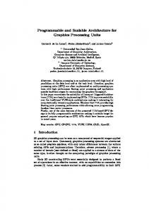
FIG. 1. 共a兲 Nonlocal transversal interaction. 共b兲 Naive linear nearest neighbor transversal interaction showing the propagation of errors resulting from the failure of a single swap gate, leading to two errors in both logical qubits. 共c兲 The first four time steps of a bilinear fault-tolerant transversal interaction between two sets of three physical qubits. The remaining three steps are the time reverse of the first three steps.

any quantum computer based around a single, global, serial interaction or transport mechanism is not scalable in the sense that it could never perform an arbitrarily large quantum computation. The purpose of this paper is to present a long-range coupling mechanism for superconducting flux qubits that can be used to couple many pairs of qubits together in parallel in a manner suited to the construction of an arbitrarily large faulttolerant quantum computer. In Sec. II, we review the coupling mechanism of Refs. 1 and 23, and extend it to allow long-range coupling in Sec. III. In Sec. IV, we firstly describe a simple, yet scalable, flux qubit architecture based on this interaction, but not taking full advantage of it, then a more complicated architecture with a better threshold error rate, though much more difficult to build. Finally, Sec. V concludes with a summary of results and a description of further work. II. COUPLING FLUX QUBITS

Before discussing our coupling mechanism, a few words elaborating exactly why long-range interactions are advantageous are in order. Essentially, the problem lies in the need to perform transversal multiple logical qubit gates, as shown in Fig. 1共a兲. If long-range interactions are available, two logical qubits each comprised of n physical qubits can be transversely interacted in a single time step using n gates. If we now try to do the same thing on a linear nearest neighbor architecture using swap gates prior to the necessary gates to perform the transversal interaction, we immediately run into a serious problem. A single swap gate failure can lead to two

FIG. 2. Coupling scheme as proposed in Ref. 1, including circuit symbols and orientations.

errors in a single logical qubit as shown in Fig. 1共b兲. Under normal circumstances, two or more errors in a single logical qubit are not correctable. A solution to this dilemma that avoids the need to resort to a multiple error correcting code is shown in Fig. 1共c兲, where a second line of placeholder qubits has been added. Now swap gates never simultaneously touch two qubits that are both part of logical qubits. Note that the first three steps of Fig. 1共c兲 need to be repeated, time reversed, to return the qubits to their original configuration. We can now see that to interact two n-qubit logical qubits transversely and fault tolerantly using only nearest neighbor interactions, using the scheme described, we need 4n qubits, 2n2 + n gates, and 2n + 1 time steps with 2n2 locations where data qubits are left idle. For all of this additional machinery to result in a circuit with the same reliability as the nonlocal case, every individual component must be significantly more reliable. This is the origin of the lower thresholds quoted in the Introduction for ever more constrained architectures. With the above motivation in mind, we proceed to the discussion of coupling superconducting flux qubits. Coherent oscillations of the state of a superconducting flux qubit were first demonstrated at Delft in 2003.46 A number of other institutions are also developing flux qubit technology, including Berkeley,23 NEC,47,48,58 RIKEN,49,50 NTT,51 and IPHT.52 A flux qubit is essentially a superconducting ring interrupted by typically three Josephson junctions with clockwise and anticlockwise persistent currents forming the basis of an effective two level quantum system. For an up-to-date review of superconducting qubit theory in general, including flux qubits, see Ref. 53. The coupling scheme as proposed in Ref. 1 is shown, somewhat simplified, in Fig. 2. Let K0 denote the strength of the direct inductive coupling between the qubits, M qq the mutual inductance of the qubits, and 兩Iq兩 the magnitude of the qubit circulating current. Note that in Ref. 1, the algebraic analysis was done with potentially different current magni共2兲 tudes 兩I共1兲 q 兩 and 兩Iq 兩, but the numerical analysis was done 共1兲 共2兲 with 兩Iq 兩 = 兩Iq 兩 = 0.48 ␮A. The above quantities are related by K0 = 2M qqI2q. Let Ks denote the strength of the coupling mediated by the superconducting quantum interference device 共SQUID兲, M qs the mutual inductance between either of the qubits and the SQUID, J the circulating current in the SQUID, ⌽s the flux through the SQUID, and Ib the SQUID bias current. These are related by 2 2 Iq Ks = 2M qs

冉 冊 ⳵J ⳵⌽s

.

共1兲

Ib

In the slowly varying and high resistance limit of the junctions, we can write

174507-2

PHYSICAL REVIEW B 76, 174507 共2007兲

LONG-RANGE COUPLING AND SCALABLE ARCHITECTURE… L
nH 5

4

3

FIG. 3. Extending coupling scheme, including circuit symbols, orientations, and dimensions. All wires are 0.75 ␮m wide and 0.1 ␮m thick.

L
pH

2

1

20 40 60 80 D
Μm 1

Ib = I0 sin ␥1 + I0 sin ␥2 ,

共2兲

2J = I0 sin ␥2 − I0 sin ␥1 ,

共3兲

where ␥1 and ␥2 are the phase drops across the SQUID Josephson junctions. This can be written as

␥ −␥ ⌬␥ = 2 2 1

where strained by

Ib = 2I0 sin ¯␥ cos ⌬␥ ,

共4兲

J = I0 sin ⌬␥ cos ¯␥ ,

共5兲

and

␥ +␥ ¯␥ = 1 2 2 .

⌬␥ =

These equations are con-

␲ 共⌽s − LdJ兲, ⌽0

共6兲

where L is the inductance of the coupler and ⌽s is nominally set to ⌽s = 0.45⌽0 to maximize the response of J to variations in ⌽s. Taking the partial derivative of Eqs. 共4兲–共6兲 with respect to ⌽s, we obtain

⳵Ib ⳵ = 0 = 2I0 共cos ⌬␥ sin ¯␥兲, ⳵⌽s ⳵⌽s

冋

共7兲

册

⳵J ⳵¯␥ ⳵⌬␥ = I0 − sin ¯␥ sin ⌬␥ + cos ¯␥ cos ⌬␥ , 共8兲 ⳵⌽s ⳵⌽s ⳵⌽s

冉

冊

⳵J ⳵⌬␥ ␲ . = 1−L ⳵⌽s ⳵⌽s ⌽0

共9兲

Using these equations, we can derive the expression

冉 冊 ⳵J ⳵⌽s

1 = 2L j Ib

1 − tan2 ¯␥ tan2 ⌬␥ , L 1+ 共1 − tan2 ¯␥ tan2 ⌬␥兲 2L j

440 420 400 380

2

3

4

D
mm 5

FIG. 4. The self-inductance of the coupler as a function of the length of the coupler.

results in decreased mutual inductance between the qubits, increased mutual inductance between the qubits and the coupler, increased self-inductance of the coupler, and significant capacitance structurally incorporated into the coupler. All of these effects will be investigated as well as the resultant impact on the coupling strength. Before discussing coupling strengths, we need to determine the various inductances of the new system. Figure 4 shows the self-inductance of the coupler versus coupler length D for coupler width d = 1.5 ␮m, generated using FASTHENRY, assuming superconducting aluminum wires with a penetration depth of 49 nm.54 The inset shows the short length behavior. For all lengths of interest, the coupler selfinductance is approximately given by 共356+ 0.863D / ␮m兲 pH. A small value of d is desirable to minimize L at a given length and, as we shall see, maximize the coupling strength. However, this also introduces a large capacitance, with consequences to be discussed at the end of this section. The mutual inductance of each qubit with the coupler was found to be 75 pH. We are now in a position to calculate the coupler mediated coupling strength Ks for zero bias current, done numerically for two different critical currents I0 = 0.48 and 0.16 ␮A, and shown in Fig. 5. Note the existence of optimum lengths, 700 and 2500 ␮m, respectively, a consequence of the cosine terms in L j. The coupling strength due to the mutual inductance of the qubits is shown in Fig. 6. Note that to neglect the Ks h
Ghz

共10兲

1.25 1 0.75

where L j = ⌽0 / 2␲I0 cos ⌬␥ cos ¯␥ is the Josephson inductance. This expression characterizes the tunable nature of the coupling scheme.

0.5 0.25 D
mm 1

III. LONG-RANGE COUPLING

We propose modifying the coupler as shown in Fig. 3. All dimensions are typical of the Berkeley group.23 This design

2

3

4

5

FIG. 5. The coupling strength at zero bias current 共⌽s = 0.45⌽0兲 without mutual qubit interaction versus the length of the coupler for I0 = 0.48 ␮A 共solid兲 and I0 = 0.16 ␮A 共dashed兲.

174507-3

PHYSICAL REVIEW B 76, 174507 共2007兲

FOWLER et al. Ks h
Ghz

K0
Ghz

0.4 1

0.3 0.2 0.1

0.1

Ib Ic

0 0.1 0.01

0.4

0.6

0.8

1

0.2

FIG. 8. The coupling strength as a function of the bias current with ⌽s = 0.45⌽0 and Ic = Ic共⌽s兲, using Josephson junction critical currents of I0 = 0.16 ␮A. D = 500 ␮m 共dotted兲, D = 1000 ␮m 共dashed兲, D = 2000 ␮m 共dash-dotted兲, and D = 4000 ␮m 共solid兲.

0.001 D
mm 0.2

0.4

0.6

0.8

1

FIG. 6. The strength of the direct qubit-qubit interaction due to mutual inductive coupling as a function of the length of the coupler, and thus, qubit separation.

direct mutual coupling, it is necessary for the qubits to be separated by approximately 650 ␮m, corresponding to a coupling strength approximately 3 orders of magnitude less than that induced by a coupler of length 650 ␮m. Its consequences in architecture design will be discussed in Sec. IV. The coupling strength can be reduced to zero by sufficiently increasing the bias current. It is desirable to ensure that the necessary increase is as small as possible, as the presence of a bias current, particularly one close to the critical current, is a significant source of decoherence.1,47,55 Figure 7 shows the coupling strength versus bias current for a selection of four coupler lengths. This figure uses the critical current I0 = 0.48 ␮A from Ref. 1. Clearly, particularly for long lengths, the bias current required to achieve zero coupling strength is too close to the critical current. This problem can be circumvented by reducing the critical current of the junctions to I0 = 0.16 ␮A, resulting in Fig. 8. Reducing the critical current reduces the zero bias coupling strength, lowering the ratio Ib / Ic required to achieve zero coupling strength. In principle, Fig. 8 is promising, both in terms of coupling strength and coupling length. However, the effect of the capacitance of the coupler must be determined. As a starting point, consider a single flux qubit initially prepared in a clockwise current state. Left alone, this qubit will oscillate between clockwise and anticlockwise current states at its tunneling frequency, which is typically of the order of a few Ks h
Ghz 1.25 1 0.75 0.5 0.25 Ib Ic

0 0.25

0.2

0.2

0.4

0.6

0.8

1

FIG. 7. The coupling strength as a function of the bias current with ⌽s = 0.45⌽0 and Ic = Ic共⌽s兲, using Josephson junction critical currents of I0 = 0.48 ␮A. D = 500 ␮m 共dotted兲, D = 1000 ␮m 共dashed兲, D = 2000 ␮m 共dash-dotted兲, and D = 4000 ␮m 共solid兲.

gigahertz in current devices. As seen by the coupler, by virtue of their mutual inductance, such a qubit plays the role of an alternating current source. Considering the coupler in isolation now, we wish to check that an alternating current source at one end of the coupler with amplitude A generates an alternating current of amplitude as close to A as possible at the other end. Using a lumped circuit model and discretizing the capacitive section of the coupler, deviation from perfect transmission of the order of 1% was found. This is low enough to give us confidence that the fundamental concept of the extended coupler is sound, but high enough that achieving high fidelity gates will require a closer examination of the physics of the system.56 We have also begun simulations of the complete system including silicon substrate using the commercial package HFSS. The results of these simulations and capacitive and radiative effects, in general, will be discussed in detail in a separate publication. IV. ARCHITECTURES

In quantum computing literature, the word “scalable” is, regrettably, frequently used rather loosely, and sometimes inaccurately. Ideally, as a minimum, it should only be claimed that an architecture is scalable if, in principle, an arbitrarily large number of qubits can be implemented, the number of quantum gates and measurements that can be executed simultaneously grows linearly with the number of qubits, and the physics of any one quantum gate or measurement does not depend on the total number of qubits. A simple example of such an architecture making use of the coupler described in this paper is shown, not drawn to scale, in Fig. 9共a兲. This figure shows eight qubits with three couplers around each qubit, each electrically isolated from the others, which is feasible with current layering technology. These have been drawn one on top of another. Note that one qubit of each pair of qubits in each coupler is more weakly coupled to the coupler following Ref. 23; this is indicated by the increased spacing in the figure between the qubit and the coupler. This enables readout of both qubits simultaneously using one coupler via the resonant readout scheme of Ref. 57. Also shown in the figure are current bias lines for each coupler with, for example, the group of three lines entering the couplers surrounding the top left qubit representing the current bias lines for the left, downward, and right leading couplers, respec-

174507-4

PHYSICAL REVIEW B 76, 174507 共2007兲

LONG-RANGE COUPLING AND SCALABLE ARCHITECTURE… a.)

b.)

FIG. 9. 共a兲 Simple scalable bilinear flux qubit architecture including flux lines for each coupler and qubit. As drawn, the architecture requires three layers of metal corresponding to the three couplers around each qubit. See Sec. IV for a full description of the various components of the figure. 共b兲 Topologically identical array used as the basis of Fig. 11.

achievable in most solid-state systems given the current ratios of decoherence times to gate times. Of course, the architecture of Fig. 9共a兲 does not take full advantage of the potential length of the coupler. As discussed earlier, to ensure relatively low cross-talk, from Fig. 4, qubits need to be spaced approximately 650 ␮m apart. This still gives us enough space to firstly stretch the architecture of Fig. 9共a兲 into a single line as shown in Fig. 9共b兲, then duplicate this line seven times to permit an additional layer of the seven-qubit Steane code to be used. Referring to Fig. 11, these duplicated qubits correspond to the bottom seven qubits in each group of 21. The middle row of qubits in each group of 21 corresponds to ancilla qubits used during error correction according to the scheme described in Ref. 27, with

a.)

12 mm

tively. Lastly, both the qubits and the couplers need independent flux bias lines, represented by small current loops near each of the qubits and each center of the couplers. These flux bias lines keep both the qubits and couplers at their optimal working points, and provide the pulses for single-qubit gates. Given the large potential length of each coupler, crosstalk can be neglected, and with only a small number of control lines leading to external circuitry per pair of qubits, given a sufficiently large fridge, many qubits can be accommodated. The details of how many qubits and how to include the necessary control lines and classical control machinery shall be left for a future publication. Two lines of qubits have been incorporated in the design to permit simpler error correction, resulting in a threshold two-qubit gate error rate for arbitrarily large fault-tolerant quantum computation of 1.96 ⫻ 10−6 as described in Ref. 32. Note that to use this architecture in practice, this implies the need for two-qubit gates operating with an error rate of 10−7 or less, far below what is q1 q2 q3 q4 q5 q6 q7

b.)

q1 q3 q2

5 mm

q7 q5 q6 q4

FIG. 10. To reduce the need for long-range interactions, the circuit 共a兲 taken from Ref. 27, which encodes and decodes a logical zero, was modified as shown in 共b兲 by swapping two pairs of qubits.

FIG. 11. 共Color online兲 A complete architecture for a flux qubit quantum computer. Squares represent flux qubits, lines connecting squares represent SQUID couplers, lines running away from each square represent squid bias current lines, and small dots with lines running away from them represent qubit and SQUID flux bias lines. The size of the flux qubits has been exaggerated for clarity. Red lines represent the SQUIDs and flux bias lines for the second and higher levels of error correction and logical gates.

174507-5

PHYSICAL REVIEW B 76, 174507 共2007兲

FOWLER et al.

slight modifications to reduce the range of the necessary interactions as shown in Fig. 10. The top row of qubits in each group of 21 corresponds to ancilla qubits only used during the implementation of the fault-tolerant T gate, or ␲ / 8 gate, as it is also known, which is required to ensure that the computer can perform a universal set of fault-tolerant gates. A complete description of the circuitry of this gate can be found in Ref. 32. Note that, even with all the additional control lines, the architecture requires just one wire per approximately 40 ␮m per side. The network of qubits and couplers shown in Fig. 11 enables the most efficient known nonlocal error correction scheme and fault-tolerant gates to be implemented at the lowest level. All higher levels make use of the circuitry devised for the bilinear architecture. When the threshold twoqubit error rate of this more complicated architecture was calculated, using the mathematical tools described in Ref. 32, the disappointingly low result of 6.25⫻ 10−6 was obtained— just over a factor of 3 better than the bilinear array. In short, the dominant nearest neighbor behavior of the large-scale architecture is not overcome by a single layer of nonlocal error correction and gates.

construction of complex, scalable quantum computer architectures as shown in Fig. 11. By virtue of the fact that flux qubits do not require large quantities of classical control circuitry on a chip, there are no obvious lithographic or heat dissipation barriers to the construction of such an architecture. The primary concern, as with all superconducting quantum technology, is decoherence. In the near future, we wish to look at other superconducting qubits and coupling schemes with the aim of removing all known sources of decoherence from the design. For example, in Ref. 47, a method of coupling flux qubits tunably is described that does not resort to a nonzero SQUID bias current. Furthermore, the need for large qubit separations to minimize cross-talk could, in principle, be alleviated by enclosing each qubit in a micrometer scale Meissner cage. Devising a more practical method of achieving higher qubit densities would greatly increase the utility of the proposed coupling scheme. Finally, with or without higher qubit densities, additional architecture design work is required to try to raise the threshold further, possibly by attempting to incorporate two layers of nonlocal error correction into the design. ACKNOWLEDGMENTS

V. CONCLUSION

We have described in detail a nonlocal method of coupling pairs of flux qubits and shown that it is suited to the

L. T. Plourde et al., Phys. Rev. B 70, 140501共R兲 共2004兲. M. A. Nielson and I. L. Chuang, Quantum Computation and Quantum Information 共Cambridge University Press, Cambridge, England, 2000兲. 3 P. W. Shor, Proceedings of the 35th Annual Symposium on Foundations of Computer Science, 1994 共unpublished兲, pp. 124–134. 4 L. K. Grover, Proceedings of the 28th Annual ACM Symposium on the Theory of Computing, May 1996 共unpublished兲, pp. 212– 219. 5 R. P. Feynman, Int. J. Theor. Phys. 21, 467 共1982兲. 6 S. Lloyd, Science 273, 1073 共1996兲. 7 B. M. Boghosian and W. Taylor, Physica D 120, 30 共1998兲. 8 A. T. Sornborger and E. D. Stewart, Phys. Rev. A 60, 1956 共1999兲. 9 T. Byrnes and Y. Yamamoto, Phys. Rev. A 73, 022328 共2006兲. 10 E. Farhi, J. Goldstone, S. Gutmann, J. Lapan, A. Lundgren, and D. Preda, Science 292, 472 共2001兲. 11 A. M. Childs, E. Farhi, J. Goldstone, and S. Gutmann, Quantum Inf. Comput. 2, 181 共2002兲. 12 M. C. Banuls, R. Orus, J. I. Latorre, A. Perez, and P. RuizFemenia, Phys. Rev. A 73, 022344 共2006兲. 13 T. Szkopek, V. Roychowdhury, and E. Yablonovitch, Phys. Rev. A 72, 062318 共2004兲. 14 D. S. Abrams and S. Lloyd, Phys. Rev. Lett. 83, 5162 共1999兲. 15 P. Jaksch and A. Papageorgiou, Phys. Rev. Lett. 91, 257902 共2003兲. 16 D. S. Abrams and C. P. Williams, arXiv:quant-ph/9908083 共unpublished兲. 1 B. 2

A.G.F and F.K.W would like to thank S. Oh for helpful discussions. This work was supported by a NSERC Discovery Grant and the European Union through EuroSQIP.

Y. Kitaev, Technical Report No. TR96-003, 1996 共unpublished兲. 18 M. Mosca and A. Ekert, Lect. Notes Comput. Sci. 1509, 174 共1999兲. 19 S. A. Fenner and Y. Zhang, Proceedings of the Ninth IC-EATCS Italian Conference on Theoretical Computer Science, 2005 共unpublished兲, pp. 215–227. 20 V. Subramaniam and P. Ramadevi, arXiv:quant-ph/0210095 共unpublished兲. 21 P. Wocjan and J. Yard, arXiv:quant-ph/0603069 共unpublished兲. 22 P. Bertet, I. Chiorescu, G. Burkard, K. Semba, C. J. P. M. Harmans, D. P. DiVincenzo, and J. E. Mooij, Phys. Rev. Lett. 95, 257002 共2005兲. 23 T. Hime, P. A. Reichardt, B. L. T. Plourde, T. L. Robertson, C.-E. Wu, A. V. Ustinov, and J. Clarke, Science 314, 1427 共2006兲. 24 S. H. W. van der Ploeg, A. Izmalkov, A. M. van den Brink, U. Hübner, M. Grajcar, E. Il’ichev, H.-G. Meyer, and A. M. Zagoskin, Phys. Rev. Lett. 98, 057004 共2007兲. 25 A. R. Calderbank and P. W. Shor, Phys. Rev. A 54, 1098 共1996兲. 26 A. M. Steane, Proc. R. Soc. London, Ser. A 425, 2551 共1996兲. 27 D. P. DiVincenzo and P. Aliferis, Phys. Rev. Lett. 98, 020501 共2007兲. 28 E. Knill, R. Laflamme, and W. H. Zurek, Los Alamos National Laboratory, Technical Report No. LAUR-96-2199, 1996 共unpublished兲. 29 E. Knill, arXiv:quant-ph/0410199 共unpublished兲. 30 A. M. Steane, Phys. Rev. A 68, 042322 共2003兲. 31 K. M. Svore, D. DiVincenzo, and B. Terhal, Quantum Inf. Com17 A.

174507-6

PHYSICAL REVIEW B 76, 174507 共2007兲

LONG-RANGE COUPLING AND SCALABLE ARCHITECTURE… put. 7, 297 共2007兲. A. M. Stephens, A. G. Fowler, and L. C. L. Hollenberg, arXiv:quant-ph/0702201 共unpublished兲. 33 A. M. Stephens, A. G. Fowler, and L. C. L. Hollenberg 共unpublished兲. 34 N.-J. Wu, M. Kamada, A. Natori, and H. Yasunaga, Jpn. J. Appl. Phys., Part 1 39, 4642 共2000兲. 35 R. Vrijen, E. Yablonovitch, K. Wang, H. W. Jiang, A. Balandin, V. Roychowdhury, T. Mor, and D. DiVincenzo, Phys. Rev. A 62, 012306 共2000兲. 36 B. Golding and M. I. Dykman, arXiv:cond-mat/0309147 共unpublished兲. 37 E. Novais and A. H. Castro Neto, Phys. Rev. A 69, 062312 共2004兲. 38 L. C. L. Hollenberg, A. S. Dzurak, C. Wellard, A. R. Hamilton, D. J. Reilly, G. J. Milburn, and R. G. Clark, Phys. Rev. B 69, 113301 共2004兲. 39 L. Tian and P. Zoller, Phys. Rev. A 68, 042321 共2003兲. 40 M. Friesen, P. Rugheimer, D. E. Savage, M. G. Lagally, D. W. van der Weide, R. Joynt, and M. A. Eriksson, Phys. Rev. B 67, 121301共R兲 共2003兲. 41 L. M. K. Vandersypen, R. Hanson, L. H. W. van Beveren, J. M. Elzerman, J. S. Greidanus, S. D. Franceschi, and L. P. Kouwenhoven, in Quantum Computing and Quantum Bits in Mesoscopic Systems, edited by A. J. Leggett, B. Ruggiero, and P. Silvestrini 共Kluwer Academic, Dordrecht/Plenum, New York, 2003兲. 42 P. Solinas, P. Zanardi, N. Zanghi, and F. Rossi, Phys. Rev. B 67, 121307共R兲 共2003兲. 43 V. V’yurkov and L. Y. Gorelik, J. Quantum Comput. Comput. 1, 77 共2000兲. 44 E. O. Kamenetskii and O. Voskoboynikov, in Trends in Quantum Computing Research, edited by Susan Shannon 共Nova Science, 32

New York, 2006兲. J. Q. You, J. S. Tsai, and F. Nori, Phys. Rev. Lett. 89, 197902 共2002兲. 46 I. Chiorescu, Y. Nakamura, C. J. P. M. Harmans, and J. E. Mooij, Science 299, 1869 共2003兲. 47 A. O. Niskanen, Y. Nakamura, and J.-S. Tsai, Phys. Rev. B 73, 094506 共2006兲. 48 A. O. Niskanen, K. Harrabi, F. Yoshihara, Y. Nakamura, and J.-S. Tsai, Phys. Rev. B 74, 220503共R兲 共2006兲. 49 Y.-X. Liu, L. F. Wei, J. S. Tsai, and F. Nori, Phys. Rev. Lett. 96, 067003 共2006兲. 50 M. Grajcar, Y.-X. Liu, F. Nori, and A. M. Zagoskin, Phys. Rev. B 74, 172505 共2006兲. 51 K. Kakuyanagi, T. Meno, S. Saito, H. Nakano, K. Semba, H. Takayanagi, F. Deppe, and A. Shnirman, Phys. Rev. Lett. 98, 047004 共2007兲. 52 M. Grajcar, A. Izmalkov, and E. Il’ichev, Phys. Rev. B 71, 144501 共2005兲. 53 M. R. Geller, E. J. Pritchett, A. T. Sornborger, and F. K. Wilhelm, in Manipulating Quantum Coherence in Solid State Systems, edited by M. E. Flatté and I. Tifrea 共Springer, Dordrecht, 2007兲. 54 T. E. Faber and A. B. Pippard, Proc. R. Soc. London, Ser. A 231, 336 共1955兲. 55 C. H. van der Wal, F. K. Wilhelm, C. J. P. M. Harmans, and J. E. Mooij, Eur. Phys. J. B 31, 111 共2003兲. 56 C. Hutter, A. Shnirman, Y. Makhlin, and G. Schön, Europhys. Lett. 74, 1088 共2006兲. 57 I. Serban, E. Solano, and F. K. Wilhelm, Phys. Rev. B 76, 104510 共2007兲. 58 A. O. Niskanen, K. Harrabi, F. Yoshihara, Y. Nakamura, S. Lloyd, and J. S. Tsai, Science 316, 723 共2007兲. 45

174507-7