1. INTRODUCTION. The gravity field and ocean explorer mission GOCE ... 1836) which connects the velocity derived from the GPS- .... Comparing the IIR-filter.
LONG WAVELENGTH GRAVITY FIELD DETERMINATION FROM GOCE USING THE ACCELERATION APPROACH Matthias Weigelt1 , Oliver Baur2 , Tilo Reubelt1 , Nico Sneeuw1 , and Matthias Roth1 1
Institute of Geodesy, Universit¨at Stuttgart, Geschwister-Scholl-Str. 24D, 70174 Stuttgart, Germany 2 Space Research Institute, Austrian Academy of Sciences, Schmiedlstr. 6, Graz, 8042, Austria
ABSTRACT In the GOCE (Gravity field and steady-state Ocean Circulation Explorer) mission two types of techniques are used for the recovery of the gravity field: gradiometry for the medium to short wavelengths and high-low satelliteto-satellite tracking (hl-SST) for the long wavelength features. For the latter, it is necessary to make use of GPS observations due to the limited measurement bandwidth of the gradiometer. In this contribution we focus on this part. Currently, the processing facilities derive the longwavelength features by using the energy conservation approach. We propose to use the acceleration approach, instead, as earlier studies for CHAMP showed that it offers a superior alternative. Theory suggest that the solution can be improved since gravity field information is available in all three directions whereas in case of the energy balance the information is primarily alongtrack. We show that for the low degrees such an improvement can be achieved. However, the processing is still at an early stage and further improvements are expected using improved filtering, better outlier detection and more reliable error information. The procedure aims at the optimal recovery of a GOCE-only solution which is one of the key objectives within the ESA’s Living Planet Programme. Key words: GOCE; acceleration approach; high-low SST.
1.
INTRODUCTION
The gravity field and ocean explorer mission GOCE started on March, 17 2009. The main objective is the determination of the gravity field of the Earth with a spatial resolution of ≈ 65 km corresponding to the degree 220 of a spherical harmonic development (Heiskanen and Moritz, 1967). The satellite is equipped with a gradiometer instrument which delivers the second derivative of the Earth’s gravitational potential. Due to its technical design, the gradiometer is optimized for the spectral range between approximately degree and order 50 and 250. Gravity signal higher than 250 is considered unrecoverable since the signal is covered by noise
whereas the low degree harmonics are derived using GPS -observations. The GOCE -mission uses the concept of high-low satellite-to-satellite tracking (high-low SST) for the long-wavelength part and the concept of satellite gravitational gradiometry (SGG) for the medium to short wavelength part. For the high-low concept several approaches exist in order to connect the GPS-observation to a gravity field quantity. The official GOCE user products make use of the energy balance approach (Jacobi, 1836) which connects the velocity derived from the GPSobservations by numerical differentiation to the gravitational potential. The approach was successfully applied to the CHAMP-mission by several authors, e.g. Gerlach et al. (2003); Howe et al. (2003); Han et al. (2002); Weigelt (2007) among others. Besides, other approaches exist. The celestial mechanics approach (Beutler et al., 2010; J¨aggi et al., 2010) is based on the variational equations and uses the measured position of the satellite directly. Similarly, the short arc method of Mayer G¨urr (2006) uses a linearized version of the variational equation which is then applied to short arcs in order to keep the linearization error small. The acceleration approach on the other hand applies double differentiation to the position resulting in in-situ accelerations along the orbit (Reubelt et al., 2003; Reubelt, 2009). Similarly, Ditmar and Van Eck van der Sluijs (2004) uses a variant of the approach which uses a simpler differentiation scheme. The approaches were compared by L¨ocher (2010) and Reubelt (2009) and both concluded that the energy balance approach performs poorest of all whereas the shortarc method and the acceleration approach are among the best methods. Investigations using the acceleration approach based on simulated data have also been done by Baur and Grafarend (2005). In this paper, we apply the acceleration approach to the GOCE mission in order to improve the long-wavelength part of the gravity field of the GOCE-only solution. We focus on the part of the high-low SST and neglect the gradiometer measurements. Numerical examples by several authors, e.g. Ditmar and Van Eck van der Sluijs (2004) or Reubelt (2009), showed that an improvement by a factor √ 3 is possible compared to the energy balance approach. Our results will show that an improvement till degree and order 20 seems possible. The paper starts with the methodology of the acceleration approach in section 2 and discusses the most impor-
tant steps, which are the numerical differentiation (section 2.2), the outlier detection and the robust estimation (section 2.3). The results are then shown in section 3.
2.
ACCELERATION APPROACH
The acceleration approach is based on Newton’s equation of motion in the inertial frame: ¨ = ∇V, x
(1)
¨ is the acceleration of the satellite and ∇V the where x gradient of the potential. The calculations are performed per unit mass. The approach is extensively discussed in Reubelt (2009). In order to account for third-bodies, tides and other effects, equation (1) is extended: ¨ − f 3rdBody − f Tides − f Rel − f Grav . ∇V = x
of CHAMP. Tests also showed, that the usage of this data adds primarily noise and yields a significant degradation of the low degree harmonic coefficients. However and with the further improving data processing, this might need to be reconsidered in the future. For the implementation of equation (2), it is important to bring all terms into the same frame. In the transfor¨ special care must be mation of the acceleration term x taken as inertial accelerations need to be considered in case of a rotating frame. Therefore, it is most convenient to use the inertial frame. On the other hand, the gradient of the gravity field ∇V on the left hand side is most conveniently modeled in the local north-oriented frame (LNOF). Consequently, the rotation between the LNF and the inertial frame needs to be applied: ∂V LNOF ∇V = RIE RE
(2)
On the right hand side f 3rdBody denotes the direct forces exerted by third bodies like the Sun, Moon and others, f Tides includes all tidal forces, f Rel are relativistic corrections and f Grav are all (time variable) gravitational changes which need to be reduced, e.g. dealiasing products. For the determination of the direct forces, the Sun and the Moon have been considered point masses. The positions of the bodies are calculated using the JPL ephemeris data DE405. The ratios of GM of each body with respect to GM Sun are taken from table 3.1 of Petit and Luzum (2010). They originate from Folkner et al. (2009) which is a description of the JPL ephemeris DE421. Tidal forces include the solid Earth tides, the solid Earth pole tide, the ocean pole tide, the ocean tide and the atmospheric tide. The solid Earth tides are calculated according to Petit and Luzum (2010, §6.2.1) up to a maximum degree of 4 and the permanent tide is removed resulting in a tide-free gravity field model. The ocean tide model is based on FES2004 (Letellier, 2004) and implemented in the version provided by the International Earth Rotation Service (IERS) (Petit and Luzum, 2010, §6.3) up to a maximum degree of 100 including the S1-tide. Also the solid Earth pole tide and the ocean pole tide are calculated in accordance with Petit and Luzum (2010). The atmospheric tide is based on the N1-model of Biancale and Bode (2006). Relativistic corrections f Rel are calculated according to equation (10.12) of Petit and Luzum (2010). The gravitational forces f Grav refer to short term variations of the gravity field which need to be removed due to the limited time resolution of the satellite systems. Currently, the AOD1B-Product (Flechtner, 2008) is in use. The six-hourly spherical harmonic coefficients are linearly interpolated to the time of calculation for each data point. Observations of the non-gravitational forces measured by the accelerometer are not used as the widely-accepted opinion is that the approach is insensitive to this influence. Non-gravitational forces have their major contribution at the frequency corresponding to one cycle per revolution. The remaining signal is below the sensitivity level
∂r 1 ∂V r ∂ϕ ∂V 1 r cos ϕ ∂λ
(3)
The rotation matrix RIE denotes the rotation from the Earth-fixed to the inertial frame and is done according to the IERS conventions (2010) (Petit and Luzum, 2010). The rotation from the LNOF to the Earth-fixed frame is given as: ( ) cos ϕ · cos λ − sin ϕ · cos λ − sin λ LNOF cos ϕ · sin λ − sin ϕ · sin λ cos λ , RE = sin ϕ cos ϕ 0 (4) where ϕ is the latitude, λ the longitude and r the radius of the position of the satellite. Last but not least, the gravitational potential V is developed into a spherical harmonic expansion (Heiskanen and Moritz, 1967). The unknowns are the coefficients of the expansion and are estimated in an iterative scheme using a weighted least-squares adjustment (see section 2.1). Equation (2) together with equations (3) and (4) form the mathematical model for the least-squares adjustment. Additionally to the spherical harmonic coefficients, also daily biases, amplitudes and phases for the once per revolution frequency are estimated as nuisance parameters.
2.1.
Methodology
Figure 1 gives an overview about the employed processing steps in order to get a gravity field solution over an arbitrary time span and free of a priori information. Point of departure are the kinematic position data provided by the European Space Agency, the aforementioned background models as well as Earth orientation parameters (EOP) provided by the IERS. The kinematic positions are double differentiated. Low-pass filtering for noise reduction might be included at this point or at a later stage as shown in the flowchart. The different accelerations and forces are then combined using the acceleration approach. Gross outlier have an massive influence on the quality of the gravity solution. Therefore, a threshold based outlier detection is employed in a first step. For this, the
Spectrum of differential operators ideal 9 point: Fs = 35 9 point: Fs = 30 9 point: Fs = 1 9 point − filtered
0.45
Normalized magnitude response * 103
0.4
0.35
0.3
0.25
0.2
0.15
0.1
0.05
0
Figure 1. Flowchart of the processing scheme
0
20
40 60 80 Cycle per revolution ≈ degree
100
120
Figure 2. Spectrum of the double difference operator. The black line denotes the ideal differentiator
difference between the filtered and reduced accelerations is formed with respect to an a priori field (here EGM96) and epochs with difference higher than 50 mGal are eliminated. The threshold has been determined empirically and corresponds to a position error of ≈ 10 m compared to a dynamic orbit. Considering the cm-accuracy of the kinematic orbit, this is a very weak constraint on the solution. It has also been investigated if the results depend on the choice of a the priori model but no such dependency was found. Further investigations also showed that the solution is influenced by poor observations which are below the threshold but have residuals larger than three times the global RMS after the adjustment. These still decrease the quality of the resulting gravity field significantly. In order to detect these observations an iterative scheme is employed. Based on the residuals of the adjustment, different tests are employed to detect outliers. Most notable is the area-based outlier detection which is described in more detail in section 2.3. Outliers above the three RMS-limit but below the gross outlier threshold are downweighted using their residuals. This procedure corresponds to a Huber estimator (G¨otzelmann et al., 2006). The iteration is stopped if the difference between the new and the previous solutions are below 10−3 . Normally, three iteration steps are sufficient (cf. section 2.3).
Observations affected by the warmup are removed. However, differentiation has the property of amplifying high frequency noise. Figure 2 shows the ideal differentiator and the frequency behavior of the employed differentiators. The black line denotes the ideal differentiator which is identical to a parabola since for double differentiation any signal needs to be multiplied by ω 2 in the frequency domain, where ω is the frequency. Due to the 1s sampling, the 9-point differentiator (dashed blue line) is identical to the ideal differentiator up to a frequency of 1500 cpr. Only then a damping effect is visible (not shown here). High-low SST signal is only expected till approximately 100 cpr. Thus, noise is strongly amplified and needs to be filtered. In order to remove the noise, the sophisticated approach is to design an IIR low-pass filter. This offers high flexibility in the design but needs to account for warmup effects which yields a loss of data. A simpler alternative is to use points every 30 or 35 seconds for differentiation and shift the scheme by 1 second afterwards. The magnitude response in figure 2 shows that similar filtering is achieved. Comparing the IIR-filter with this procedure, a stronger damping effect for degrees higher than 70 is visible.
2.2.
2.3.
Numerical differentiation and filtering
¨ need to be derived from the kineThe accelerations x matic positions by numerical differentiation. It is done using a Taylor differentiator (Khan and Ohba, 1999) aka. Newton-Gregory or finite central difference differentiator. Previous studies for CHAMP with a 30 second sampling showed that the 9-point Taylor differentiator performs best. The order is chosen to be n = 4, i.e. the differentiator has 2n+1 = 9 elements and a warmup of 4.
Outlier detection and robust estimation
Investigations showed that a simple threshold based outlier detection can only be used for gross outlier determination. Poor observations affect the solution significantly (cf. figure 4) but are not necessarily indicated by the variance information. In order to find these poor observations, an iterative scheme is necessary. Outliers are detected based on the residuals between the observations and the signal reconstructed from the solution. The im-
90 60
10
itg_grace03 Data set 1 Data set 2 Data set 3 Data set 4 Data set 5
0.6
30 0.5
0
10
0 0.4 −30 0.3
−60 −90 −180
−150
−120
−90
−60
−30 0 30 longitude [deg]
60
90
120
150
180
90
0.2
Geoid heights* (m)
latitude [deg]
1
0.7
−1
10
0.7 −2
10
latitude [deg]
60
0.6
30 0.5 0
−3
10
0.4
10
20
30
−90 −180
40 50 degree l
60
70
80
90
0.3
−60
−150
−120
−90
−60
−30 0 30 longitude [deg]
60
90
120
150
180
90
0.2
Figure 4. Square root of degree difference variances w.r.t. ITG-Grace03s (Mayer G¨urr, 2006) expressed in geoid heights for five iteration steps
0.7
60
latitude [deg]
0
−30
0.6
30 0.5 0 0.4
−30 0.3
−60 −90 −180
−150
−120
−90
−60
−30 0 30 longitude [deg]
60
90
120
150
180
90
0.2
stood, yet. Figure 4 shows the importance of the iteration scheme. For one month of data the solution has been iterated 5 times. In the first step, only gross outliers have been eliminated. The solution is almost 2 orders of magnitude worse than in the subsequent steps where poor observations have been identified. The iteration converged after 3 steps. Similar conclusions have also been drawn by Reubelt (2009).
200
60
Latitude [deg]
150 30 0
RESULTS
100
−30 50 −60 −90 −180
3.
0 −150
−120
−90
−60
−30 0 30 Longitude [deg]
60
90
120
150
180
The results for the GOCE solutions calculated by the acceleration approach using 61 and 181 days of data are shown in figure 5 and are denoted ACC61 and ACC181, respectively. The comparison to the time-wise GOCE so0
10
Figure 3. Outlier limits: x-coordinate, y-coordinate, zcoordinate and the number of found outliers per 5◦ × 5◦ block (from top)
−1
portant factor in the detection of the outlier is the threshold in use. Using an inertial coordinate frame, the RMS of the residuals was found to depend on the spatial location and the coordinate axis. Figure 3 shows this dependency in the first three panels for the x-, y- and z-coordinate. The RMS has been calculated for 5◦ × 5◦ blocks using all the available data in a spherical cap of 20◦ around the center of the block. Observations in a specific block deviating more than 3 times from the RMS are downweighted using the difference between the observation and the reconstructed signal of the i-th iteration step. The number of outliers found per block is shown in the bottom panel of figure 3 and indicates on the one hand specific arcs, which have been poorly determined, but also shows local concentrations. The reason for the later is not under-
Geoid heights* (m)
10
−2
10
−3
10
0
10
20
30
40 50 degree l
ITG−GRACE03s AIUB_CHAMP03S (7 years) EIGEN_CHAMP05S (5 years) GO_CONS_GCF_2_TIM (61 days) ACC61 (GOCE 61 days) ACC181 (GOCE 181 days) CHAMP − UofC (2 years) 60 70 80 90
Figure 5. Square root of degree difference variances w.r.t. ITG-Grace03s (Mayer G¨urr, 2006) expressed in geoid heights
lution GO-CONS-GCF-2-TIM (Pail et al., 2010), which is the only one that is independent of a priori information for the low degrees, suggest that an improvement is possible till degree 20. On the other hand, the GOCE solutions exhibit also a loss of accuracy in the very low degrees (2-5). The reason for this is not fully understood, yet. Possibilities are neglected co-variance information and non-gravitational forces. Further improvements are expected in the future due to optimized filtering and outlier detection. An interesting comparison is also the comparison to CHAMP . The GOCE -solutions outperform the 2-year CHAMP solution UOFC (Weigelt, 2007) for degrees higher than 3 and the 5 and 7 year CHAMP solutions EIGEN-CHAMP05s (Flechtner et al., 2010) and AIUBCHAMP03s (Prange et al., 2010) for degrees higher than 45 due to the lower orbit of GOCE. In the low degrees the long-term solutions of CHAMP are still significantly better.
4.
CONCLUSION
It has been shown that the acceleration approach offers an improvement to the energy balance approach and thus poses an interesting alternative to the current processing strategy. The 61 day solution outperforms already the 2 and in the high degrees the 5 and 7 year solutions from CHAMP primarily due to the lower orbit of GOCE . Currently, the solutions exhibit problems in the low degree harmonics 2-5. The reason for this is not yet understood. Possible causes are neglected covariance information and non-gravitational forces. Further improvements are also expected by refined filtering and outlier detection strategies. The former is expected to yield an improvement to the high degrees as currently to much signal has been filtered for degrees higher than 50.
REFERENCES Baur, O., and E. Grafarend, High-performance GOCE gravity field recovery from gravity gradient tensor invariants and kinematic orbits information, in Observation of the Earth System from Space, edited by J. Flury, R. Rummel, C. Reigber, M. Rothacher, G. Boedecker, and U. Schreiber, pp. 239–253, Springer, 2005. Beutler, G., A. J¨aggi, L. Mervart, and U. Meyer, The celestial mechanics approach: theoretical foundations, J. Geod., 84(10), 605–624, doi:10.1007/s00190-0100401-7, 2010. Biancale, R., and A. Bode, Mean Annual and Seasonal Atmospheric Tide Models Based on 3-hourly and 6-hourly ECMWF Surface Pressure Data, Scientific Technical Report STR 06/01, GeoForschungsZentrum Potsdam, doi:10.2312/GFZ.b103-06011, 2006. Ditmar, P., and A. Van Eck van der Sluijs, A technique for modeling the Earth’s gravity field on the basis of satellite accelerations, J. Geod., 78, 12–33, doi: 10.1007/s00190-003-0362-1, 2004.
Flechtner, F., A long-term model for non-tidal atmospheric and oceanic mass redistributions and its implications on LAGEOS-derived solutions of Earth’s oblateness, Scientific Technical Report STR 08/12, GeoForschungszentrum Potsdam, doi: 10.2312/GFZ.b103-08123, 2008. Flechtner, F., C. Dahle, K. Neumayer, R. K¨onig, and C. F¨orste, The release 04 champ and grace eigen gravity field models, in System Earth via GeodeticGeophysical Space Techniques, edited by F. Flechtner, T. Gruber, A. G¨untner, M. Mandea, M. Rothacher, T. Sch¨one, and J. Wickert, 2010. Folkner, W., J. Williams, and D. Boggs, The Planetary and Lunar Ephemeris DE 421, Tech. rep., IPN Progress Report 42-178, 2009. ˇ Gerlach, C., N. Sneeuw, P. Visser, and D. Svehla, CHAMP gravity field recovery using the energy balance approach, Adv. Geosci., 1, 73–80, 2003. G¨otzelmann, M., W. Keller, and T. Reubelt, Gross erorr compensation for gravity filed analysis based on kinematic orbit data, J. Geod., 80(4), 184–198, doi: 10.1007/s00190-006-0061-9, 2006. Han, S., Ch. Jekeli, and C. Shum, Efficient gravity field recovery using in situ disturbing potential observables from CHAMP, Geophys. Res. Lett., 29(16), 36–1–36– 4, doi:10.1029/2002GL015180, 2002. Heiskanen, W., and H. Moritz, Physical geodesy, W.H. Freeman and Company San Francisco, 1967. Howe, E., L. Stenseng, and C. Tscherning, Analysis of one month of CHAMP state vector and accelerometer data for the recovery of the gravity potential, Adv. Geosci., 1, 1–4, 2003. ¨ Jacobi, C., Uber ein neues Integral f¨ur den Fall der drei K¨orper, wenn die Bahn des st¨orenden Planeten kreisf¨ormig angenommen und die Masse des gest¨orten vernachl¨assigt wird., Monthly reports of the Berlin Academy, 1836. J¨aggi, A., L. Prange, and U. Hugentobler, Impact of covariance information of kinematic positions on orbit reconstruction and gravity field recovery, Adv. Space Res., In Press, Corrected Proof, –, doi: 10.1016/j.asr.2010.12.009, 2010. Khan, I., and R. Ohba, Closed-form expressions for the finite difference approximations of first and higher derivaties based on Taylor series, J. Comput. Appl. Math., 107(2), 179–193, doi:10.1016/S03770427(99)00088-6, 1999. Letellier, T., Etude des ondes de mari`ne sur les plateux continentaux, FES2004 - Road to the data and the thesis (in French)., Th`ese doctorale, Universit`e de Toulouse III, Ecole Doctorale des Sciences de l’Univers, de l’Environnement et de l’Espace, 2004. L¨ocher, A., M¨oglichkeiten der Nutzung kinematischer Satellitenbahnen zur Bestimmung des Gravitationsfeldes der Erde, Ph.D. thesis, Rheinische FriedrichWilhelms-Universit¨at zu Bonn, 2010.
Mayer G¨urr, T., Gravitationsfeldbestimmung aus der Analyse kurzer Bahnb¨ogen am Beispiel der Satellitenmissionen CHAMP und GRACE, Ph.D. thesis, Rheinische Friedrich-Wilhelms-Universit¨at zu Bonn, 2006. Pail, R., H. Goiginger, R. Mayrhofer, W.-D. Schuh, J. Brockmann, I. Krasbutter, E. Hoeck, and T. Fecher, Goce gravity field model derived from orbit and gradiometry data applying the time-wise method, in Proceedings of the ESA Living Planet Symposium, 28 June - 2 July 2010, Bergen, Norway, 2010. Petit, G., and B. Luzum, IERS Conventions (2010), Tech. Rep. 36, IERS, Frankfurt am Main, Verlag des Bundesamts f¨ur Kartographie und Geod¨asie, updated version from 20th July 2006, 2010. Prange, L., A. J¨aggi, G. Beutler, U. Meyer, L. Mervart, R. Dach, and H. Bock, Aiub-champ03s: A gravity field model from eight years of champ gps data, paper in preparation, 2010. Reubelt, T., Harmonische Gravitationsfeldanalyse aus GPS-vermessenen kinematischen Bahnen niedrig fliegender Satelliten vom Typ CHAMP, GRACE und GOCE mit einem hoch aufl¨osenden Beschleunigungsansatz, Ph.D. thesis, Institute of Geodesy, University of Stuttgart, 2009. Reubelt, T., G. Austen, and E. Grafarend, Harmonic analysis of the Earth´s gravitational field by means of semicontinuous ephemerides of a low Earth orbiting GPStracked satellite. Case study: CHAMP, J. Geod., 77(5– 6), 257–278, doi:10.1007/s00190-003-0322-9, 2003. Weigelt, M., Global and local gravity field recovery from satellite-to-satellite tracking, Ph.D. thesis, University of Calgary, http://www.geomatics.ucalgary.ca/graduatetheses, 2007.