Longest Common Subsequence in at Least k Length Order ...

arXiv:1609.03668v2 [cs.DS] 29 Oct 2016

Longest Common Subsequence in at Least k Length Order-isomorphic Substrings∗ Yohei Ueki1 , Diptarama1 , Masatoshi Kurihara1 , Yoshiaki Matsuoka2 , Kazuyuki Narisawa1 , Ryo Yoshinaka1 , Hideo Bannai2 , Shunsuke Inenaga2 , and Ayumi Shinohara1 1

Graduate School of Information Sciences, Tohoku University, Sendai, Japan {yohei ueki,diptarama,masatoshi kurihara}@shino.ecei.tohoku.ac.jp {narisawa,ry,ayumi}@ecei.tohoku.ac.jp 2 Department of Informatics, Kyushu University, Fukuoka, Japan {yoshiaki.matsuoka, bannai, inenaga}@inf.kyushu-u.ac.jp

Abstract We consider the longest common subsequence (LCS) problem with the restriction that the common subsequence is required to consist of at least k length substrings. First, we show an O(mn) time algorithm for the problem which gives a better worst-case running time than existing algorithms, where m and n are lengths of the input strings. Furthermore, we mainly consider the LCS in at least k length order-isomorphic substrings problem. We show that the problem can also be solved in O(mn) worst-case time by an easy-to-implement algorithm.

1

Introduction

The longest common subsequence (LCS) problem is fundamental and well studied in computer science. The most common application of the LCS problem is measuring similarity between strings, which can be used in many applications such as the diff tool, the time series data analysis [12], and in bioinformatics. One of the major disadvantages of LCS as a measure of similarity is that LCS cannot consider consecutively matching characters effectively. For example, for strings X = ATGG, Y = ATCGGC and Z = ACCCTCCCGCCCG, ATGG is the LCS of X and Y , which is also the LCS of X and Z. Benson et al. [2] introduced the longest common subsequence in k length substrings (LCSk ) problem, where the subsequence needs to be a concatenation of k length substrings of given strings. For example, for strings X = ATCTATAT and Y = TAATATCC, TAAT is an LCS2 since X[4 : 5] = Y [1 : 2] = TA and X[7 : 8] = Y [5 : 7] = AT, and no longer one exists. They showed a quadratic time algorithm for it, and Deorowicz and Grabowski [7] proposed several algorithms, such as a quadratic worst-case time algorithm for unbounded k and a fast algorithm on average. ∗

To appear in Proc. SOFSEM 2017.

1

Paveti´c et al. [15] considered the longest common subsequence in at least k length substrings (LCSk+ ) problem, where the subsequence needs to be a concatenation of at least k length substrings of given strings. They argued that LCSk+ would be more appropriate than LCSk as a similarity measure of strings. For strings X = ATTCGTATCG, Y = ATTGCTATGC, and Z = AATCCCTCAA, LCS 2 (X, Y ) = LCS 2 (X, Z) = 4, where LCS 2 (A, B) denotes the length of an LCS2 between A and B. However, it seems that X and Y are more similar than X and Z. Instead, if we consider LCS2+ , we have LCS 2+ (X, Y ) = 6 > 4 = LCS 2+ (X, Z), that better fits our intuition. The notion of LCSk+ is applied to bioinformatics [16]. Paveti´c et al. showed that LCSk+ can be computed in O(m + n + r log r + r log n) time, where m, n are lengths of the input strings and r is the total number of matching k length substring pairs between the input strings. Their algorithm is fast on average, but in the worst case, the running time is O(mn log(mn)). Independently, Benson et al. [2] proposed an O(kmn) worst-case time algorithm for the LCSk+ problem. In this paper, we first propose an algorithm to compute LCSk+ in O(mn) worst-case time by a simple dynamic programming. Secondly, we introduce the longest common subsequence in at least k length order-isomorphic substrings (op-LCSk+ ) problem. Orderisomorphism is a notion of equality of two numerical strings, intensively studied in the order-preserving matching problem1 [13, 14]. op-LCSk+ is a natural definition of similarity between numerical strings, and can be used in time series data analysis. The op-LCSk+ problem cannot be solved as simply as the LCSk+ problem due to the properties of the order-isomorphism. However, we will show that the op-LCSk+ problem can also be solved in O(mn) worst-case time by an easy-to-implement algorithm, which is one of the main contributions of this paper. Finally, we report experimental results.

2

Preliminaries

We assume that all strings are over an alphabet Σ. The length of a string X = (X[1], X[2], · · · , X[n]) is denoted by |X| = n. A substring of X beginning at i and ending at j is denoted by X[i : j] = (X[i], X[i + 1], · · · , X[j − 1], X[j]). We denote Xhi, +li = X[i : i+l −1] and Xhj, −li = X[j −l +1 : j]. Thus Xhi, +li = Xhi+l −1, −li. We write X[: i] and X[j :] to denote the prefix X[1 : i] and the suffix X[j : n] of X, respectively. Note that X[: 0] is the empty string. The reverse of a string X is denoted by X R , and the operator · denotes the concatenation. We simply denote a string X = (X[1], X[2], · · · , X[n]) as X = X[1]X[2] · · · X[n] when clear from the context. We formally define the LCSk+ problem as follows. Definition 1 (LCSk+ problem [2, 15]2 ). Given two strings X and Y of length m and n, respectively, and an integer k ≥ 1, we say that Z is a common subsequence in at least k length substrings of X and Y , if there exist i1 , · · · , it and j1 , · · · , jt such that Xhis , +ls i = Y hjs , +ls i = Zhps , +ls i and ls ≥ k for 1 ≤ s ≤ t, and is + ls ≤ is+1 , 1

Since the problem is motivated by the order-preserving matching problem, we abbreviate it to the op-LCSk+ problem. 2 The formal definition given by Paveti´c et al. [15] contains a minor error, i.e., they do not require that each chunk is identical, while Benson et al. [2] and we do (confirmed by F. Paveti´c, personal communication, October 2016).

2

js + ls ≤ js+1 and ps+1 = ps + ls for 1 ≤ s < t, p1 = 1 and |Z| = pt + lt − 1. The longest common subsequence in at least k length substrings (LCSk+ ) problem asks for the length of an LCSk+ of X and Y . Remark that the LCS1+ problem is equivalent to the standard LCS problem. Without loss of generality, we assume that n ≥ m through the paper. Example 1. For strings X = acdbacbc and Y = aacdabca, Z = acdbc is the LCS2+ of X and Y , since Xh1, +3i = Y h2, +3i = acd = Zh1, +3i and Xh7, +2i = Y h6, +2i = bc = Zh4, +2i. Note that the standard LCS of X and Y is acdabc. The main topic of this paper is to give an efficient algorithm for computing the longest common subsequence under order-isomorphism, defined below. Definition 2 (Order-isomorphism [13, 14]). Two strings S and T of the same length l over an ordered alphabet are order-isomorphic if S[i] ≤ S[j] ⇐⇒ T [i] ≤ T [j] for any 1 ≤ i, j ≤ l. We write S ≈ T if S is order-isomorphic to T , and S 6≈ T otherwise. Example 2. For strings S = (32, 40, 4, 16, 27), T = (28, 32, 12, 20, 25) and U = (33, 51, 10, 22, 42), we have S ≈ T , S 6≈ U , and T 6≈ U . Definition 3 (op-LCSk+ problem). The op-LCSk+ problem is defined as the problem obtained from Definition 1 by replacing the matching relation Xhis , +ls i = Y hjs , +ls i = Zhps , +ls i with order-isomorphism Xhis , +ls i ≈ Y hjs , +ls i ≈ Zhps , +ls i. Example 3. For strings X = (14, 84, 82, 31, 74, 68, 87, 11, 20, 32) and Y = (21, 64, 2, 83, 73, 51, 5, 29, 7, 71), Z = (1, 3, 2, 31, 74, 68, 87) is an op-LCS3+ of X and Y since Xh1, +3i ≈ Y h3, +3i ≈ Zh1, +3i and Xh4, +4i ≈ Y h7, +4i ≈ Zh4, +4i. The op-LCSk+ problem does not require that (Xhi1 , +l1 i·Xhi2 , +l2 i· · · · ·Xhit , +lt i) ≈ (Y hj1 , +l1 i · Y hj2 , +l2 i · · · · · Y hjt , +lt i). Therefore, the op-LCS1+ problem makes no sense. Note that the op-LCSk+ problem with this restriction is NP-hard already for k = 1 [3].

3

The LCSk+ Problem

In this section, we show that the LCSk+ problem can be solved in O(mn) time by dynamic programming. We define Match(i, j, l) = 1 if Xhi, −li = Y hj, −li, and 0 otherwise. Let C[i, j] be the length of an LCSk+ of X[: i] and Y [: j], and Ai,j = {C[i − l, j − l] + l · Match(i, j, l) : k ≤ l ≤ min{i, j}}. Our algorithm is based on the following lemma. Lemma 1 ([2]). For any k ≤ i ≤ m and k ≤ j ≤ n, C[i, j] = max ({C[i, j − 1], C[i − 1, j]} ∪ Ai,j ) , and C[i, j] = 0 otherwise.

3

(1)

The naive dynamic programming algorithm based on Equation (1) takes O(m2 n) time, because for each i and j, the naive algorithm for computing max Ai,j takes O(m) time assuming n ≥ m. Therefore, we focus on how to compute max Ai,j in constant time for each i and j in order to solve the problem in O(mn) time. It is clear that if Match(i, j, l1 ) = 0 then Match(i, j, l2 ) = 0 for all valid l2 ≥ l1 , and C[i0 , j 0 ] ≥ C[i0 − l0 , j 0 − l0 ] for all valid i0 , j 0 and l0 > 0. Therefore, in order to compute max Ai,j , it suffices to compute maxk≤l≤L[i,j] {C[i − l, j − l] + l}, where L[i, j] = max{l : Xhi, −li = Y hj, −li}. We can compute L[i, j] for all 0 ≤ i ≤ m and 0 ≤ j ≤ n in O(mn) time by dynamic programming because the following equation clearly holds: ( L[i − 1, j − 1] + 1 (if i, j > 0 and X[i] = Y [j]) L[i, j] = (2) 0 (otherwise). Next, we show how to compute maxk≤l≤L[i,j] {C[i − l, j − l] + l} in constant time for each i and j. Assume that the table L has already been computed. Let M [i, j] = maxk≤l≤L[i,j] {C[i − l, j − l] + l} if L[i, j] ≥ k, and −1 otherwise. Lemma 2. For any 0 ≤ i ≤ m and 0 ≤ j ≤ n, if L[i, j] > k then M [i, j] = max{M [i − 1, j − 1] + 1, C[i − k, j − k] + k}. Proof. Let l = L[i, j]. Since L[i, j] > k, we have L[i − 1, j − 1] = l − 1 ≥ k, and M [i−1, j −1] 6= −1. Therefore, M [i−1, j −1] = maxk≤l0 ≤l−1 {C[i−1−l0 , j −1−l0 ]+l0 } = maxk+1≤l0 ≤l {C[i − l0 , j − l0 ] + l0 } − 1. Hence, M [i, j] = maxk≤l0 ≤l {C[i − l0 , i − l0 ] + l0 } = max{M [i − 1, j − 1] + 1, C[i − k, j − k] + k}. By Lemma 2 and the definition of M [i, j], we have   max{M [i − 1, j − 1] + 1, C[i − k, j − k] + k} (if L[i, j] > k) M [i, j] = C[i − k, j − k] + k (if L[i, j] = k)   −1 (otherwise).

(3)

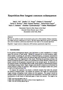
Equation (3) shows that each M [i, j] can be computed in constant time if L[i, j], M [i − 1, j − 1], and C[i − k, j − k] have already been computed. We can fill in tables C, L and M of size (m + 1) × (n + 1) based on Equations (1), (2) and (3) in O(mn) time by dynamic programming. An example of computing LCS3+ is shown in Fig. 1(a). We note that LCSk+ itself (not only its length) can be extracted from the table C in O(m + n) time, by tracing back in the same way as the standard dynamic programming algorithm for the standard LCS problem. Our algorithm requires O(mn) space since we use three tables of size (m + 1) × (n + 1). Note that if we want to compute only the length of an LCSk+ , the space complexity can be easily reduced to O(km). Hence, we get the following theorem. Theorem 1. The LCSk+ problem can be solved in O(mn) time and O(km) space.

4

a b c b c d e f

4 0 9 6 2 0 3 1

0

1

2

3

4

5

6

7

8

0

1

2

3

4

5

6

7

8

0 0

0

0

0

0

0

0

0

0

0 0

0

0

0

0

0

0

0

0

a 1 0 b 2 0

0

0

0

0

0

0

0

0

0

0

0

0

0

0

0

0

0

0

0

0

0

0

0

0

5 1 0 1 2 0

0

2

2

2

2

2

2

2

c 3 0 d 4 0

0

0

3

3

3

3

3

3

0

2

2

2

2

2

2

2

0

0

3

3

3

3

3

3

3 3 0 8 4 0

0

2

2

2

2

2

4

4

7 5 0 2 6 0

0

2

2

4

4

4

4

5

0

2

2

4

5

5

5

5

e 5 0 f 6 0

0

0

3

3

3

3

4

4

0

0

3

3

3

3

4

6

(a) Table C for the LCS3+ problem

(b) Table C for the op-LCS2+ problem

Figure 1: Examples of computing LCS3+ and op-LCS2+

4

The op-LCSk+ Problem

In this section, we show that the op-LCSk+ problem can be solved in O(mn) time as well as the LCSk+ problem. We redefine C[i, j] to be the length of an op-LCSk+ of X[: i] and Y [: j], and Match(i, j, l) = 1 if Xhi, −li ≈ Y hj, −li, and 0 otherwise. It is easy to prove that Equation (1) also holds with respect to the order-isomorphism. However, the op-LCSk+ problem cannot be solved as simply as the LCSk+ problem because Equations (2) and (3) do not hold with respect to the order-isomorphism, as follows. For two strings A, B of length l such that A ≈ B, and two characters a, b such that A · a 6≈ B · b, the statement “(A · a)[i :] 6≈ (B · b)[i :] for all 1 ≤ i ≤ l + 1” is not always true. For example, for strings A = (32, 40, 4, 16, 27), B = (28, 32, 12, 20, 25), A0 = A · (41) and B 0 = B · (26), we have A ≈ B, A0 6≈ B 0 , and A0 [3 :] ≈ B 0 [3 :]. Moreover, for A00 = A · (15) and B 00 = B · (22), we have A00 [5 :] ≈ B 00 [5 :]. These examples show that Equations (2) and (3) do not hold with respect to the order-isomorphism. Therefore, we must find another way to compute maxk≤l0 ≤l {C[i − l0 , j − l0 ] + l0 }, where l = max{l0 : Xhi, −l0 i ≈ Y hj, −l0 i} in constant time. First, we consider how to find max{l : Xhi, −li ≈ Y hj, −li} in constant time. We define the order-preserving longest common extension (op-LCE) query on strings S1 and S2 as follows. Definition 4 (op-LCE query). Given a pair (S1 , S2 ) of strings, an op-LCE query is a pair of indices i1 and i2 of S1 and S2 , respectively, which asks opLCE S1 ,S2 [i1 , i2 ] = max{l : S1 hi1 , +li ≈ S2 hi2 , +li}. Since max{l : Xhi, −li ≈ Y hj, −li} = opLCE X R ,Y R [m − i + 1, n − j + 1], we can find max{l : Xhi, −li ≈ Y hj, −li} by using op-LCE queries on X R and Y R . Therefore, we focus on how to answer op-LCE queries on S1 and S2 in constant time with at most O(|S1 ||S2 |) time preprocessing. Hereafter we write opLCE [i1 , i2 ] for opLCE S1 ,S2 [i1 , i2 ] fixing two strings S1 and S2 . If S1 and S2 are strings over a polynomially-bounded integer alphabet {1, · · · , (|S1 | + |S2 |)c } for an integer constant c, op-LCE queries can be answered in O(1) time and O(|S1 | + |S2 |) space with O((|S1 | + |S2 |) log2 log(|S1 | + |S2 |)/ log log log(|S1 | + |S2 |)) time preprocessing, by using the incomplete generalized op-suffix-tree [6] of S1 and S2 and 5

finding the lowest common ancestor (LCA) [1] in the op-suffix-tree. The proof is similar to that for LCE queries in the standard setting [10]. However, implementing the incomplete generalized op-suffix-tree is quite difficult. Therefore, we introduce another much simpler method to answer op-LCE queries in O(1) time with O(|S1 ||S2 |) time preprocessing. In a preprocessing step, our algorithm fills in the table opLCE [i1 , i2 ] for all 1 ≤ i1 ≤ |S1 | and 1 ≤ i2 ≤ |S2 | in O(|S1 ||S2 |) time. Then, we can answer op-LCE queries in constant time. In the preprocessing step, we use the Z-algorithm [10, 11] that calculates the following table efficiently. Definition 5 (Z-table). The Z-table ZS of a string S is defined by ZS [i] = max{l : Sh1, +li ≈ Shi, +li} for each 1 ≤ i ≤ |S|. By definition, we have  opLCE [i1 , i2 ] = min Z(S1 ·S2 )[i1 :] [|S1 | − i1 + i2 + 1], |S1 | − i1 + 1 .

(4)

If we use the Z-algorithm and Equation (4) naively, it takes O((|S1 | + |S2 |)2 log(|S1 | + |S2 |)) time to compute opLCE [i1 , i2 ] for all 1 ≤ i1 ≤ |S1 | and 1 ≤ i2 ≤ |S2 |, because the Z-algorithm requires O(|S| log |S|) time to compute ZS for a string S. We extend the Z-algorithm to compute ZS[i:] for all 1 ≤ i ≤ |S| totally in O(|S|2 ) time. In order to verify the order-isomorphism in constant time with preprocessing, Hasan et al. [11] used tables called Prev S and Next S . For a string S where all the characters are distinct5 , Prev S and Next S are defined as Prev S [i] = j if there exists j = argmax{S[k] : S[k] < S[i]}, and

−∞ otherwise

1≤k S[i]}, and

∞ otherwise

1≤k S 0 [j] do s.pop(); if s = ∅ then Prev [S 0 [j] − i + 1] ← −∞; else Prev [S 0 [j] − i + 1] ← s.top() − i + 1; s.push(S 0 [j]); if S 00 [j] ≥ i then while t 6= ∅ and t.top() > S 00 [j] do t.pop(); if t = ∅ then Next[S 00 [j] − i + 1] ← ∞; else Next[S 00 [j] − i + 1] ← t.top() − i + 1; t.push(S 00 [j]); return (Prev , Next); Function Z-function(S, i1 , S 0 , S 00 ) (Prev , Next) ← preprocess(S, i1 , S 0 , S 00 ); S ← S[i1 :]; Do the same operations described in line 3-17 of Algorithm 4 in [11]; return Z; Function preprocess-opLCE(S1 , S2 ) Let opLCE be a table of size |S1 | × |S2 |; S ← S1 · S2 ; Let S 0 and S 00 be stably sorted positions of S with respect to their elements in ascending and descending order, respectively; for i1 ← 1 to |S1 | do Z ← Z-function(S, i1 , S 0 , S 00 ); for i2 ← 1 to |S2 | do n o opLCE [i1 , i2 ] ← min Z[|S1 | − i1 + i2 + 1], |S1 | − i1 + 1 ; return opLCE ;

7

Algorithm 2: The algorithm for the op-LCSk+ problem Input: A string X of length m, a string Y of length n, and an integer k Output: The length of an op-LCSk+ between X and Y 1 Let C be a table of size (m + 1) × (n + 1) initialized by 0; 2 Let Ri for −n + k ≤ i ≤ m − k be semi-dynamic RMQ data structures; 3 opLCE ← preprocess-opLCE(X R , Y R ); 4 for i ← 0 to m − k do 5 if i < k then n0 ← n − k; 6 else n0 ← k − 1; 7 for j ← 0 to n0 do Ri−j .prepend(C[i, j] − min{i, j});

14

for i ← k to m do for j ← k to n do l ← opLCE [m − i + 1, n − j + 1]; if l ≥ k then M ← Ri−j .rmq(k, l) + min{i, j}; else M ← 0; C[i, j] ← max{C[i, j − 1], C[i − 1, j], M }; Ri−j .prepend(C[i, j] − min{i, j});

15

return C[m, n];

8 9 10 11 12 13

in the stack, and pop() removes it. Algorithm 1 takes O(|S1 ||S2 |) time as discussed above. The total space complexity is O(|S1 ||S2 |) because the Z-algorithm requires linear space [11], and the table opLCE needs O(|S1 ||S2 |) space. Hence, we have the following lemma. Lemma 3. op-LCE queries on S1 and S2 can be answered in O(1) time and O(|S1 ||S2 |) space with O(|S1 ||S2 |) time preprocessing. Let opLCE(i, j) be the answer to the op-LCE query on X R and Y R with respect to the index pair (i, j). We consider how to find the maximum value of C[i − l, j − l] + l for k ≤ l ≤ opLCE(m − i + 1, n − j + 1) in constant time. We use a semi-dynamic range maximum query (RMQ) data structure that maintains a table A and supports the following two operations: • prepend(x): add x to the beginning of A in O(1) amortized time. • rmq(i1 , i2 ): return the maximum value of A[i1 : i2 ] in O(1) time.

The details of the semi-dynamic RMQ data structure will be given in Section 5. By using the semi-dynamic RMQ data structures and the following obvious lemma, we can find maxk≤l≤opLCE(m−i+1,n−j+1) {C[i − l, j − l] + l} for all 1 ≤ i ≤ m and 1 ≤ j ≤ n in totally O(mn) time. Lemma 4. We may assume that i ≥ j without loss of generality. Let A[l] = C[i − l][j − l] + l and A0 [l] = C[i − l][j − l] − j + l for each 1 ≤ l ≤ j. For any 1 ≤ i1 , i2 ≤ |A|, we have maxi1 ≤l≤i2 A[l] = (maxi1 ≤l≤i2 A0 [l]) + j and argmaxi1 ≤l≤i2 A[l] = argmaxi1 ≤l≤i2 A0 [l].

8

rmq(2,4)

rmq(5,7)

-∞

1

2

3

4

5

6

7

8

𝑋=

4

6

5

7

3

4

5

3

𝑌=

1

2

4

5

9

10

11

15

𝐸= 0 1 2 1 3 4 3 1 0 5 6 7 6 5 0 8 𝐷= 0 1 2 1 2 3 2 1 0 1 2 3 2 1 0 1

rmq1 2,5 + 1

rmq1(9,11)

0

lca(2,4)

1 4

5 3

8 3

2 6 3 5 6 4

lca(5,7)

4 7 7 5

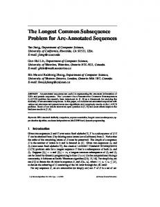
Figure 2: An example of searching for the RMQ by using a 2d-Min-Heap and the ±1RMQ algorithm [1]. The tree shows the 2d-Min-Heap of X = (4, 6, 5, 7, 3, 4, 5, 3) represented by arrays E and D. The gray node 8 in the tree and gray numbers in the table are added when the last character X[8] = 3 is processed. The boxes with the dashed lines show the answers of RMQs rmq(2, 4) and rmq(5, 7). Algorithm 2 shows our algorithm to compute op-LCSk+ . An example of computing op-LCS2+ is shown in Fig. 1(b). As discussed above, the algorithm runs in O(mn) time. Each semi-dynamic RMQ data structure requires linear space and a total of O(mn) elements are maintained by the semi-dynamic RMQ data structures. Therefore, the total space of semi-dynamic RMQ data structures is O(mn). Consequently, the total space complexity is O(mn). Hence, we have the following theorem. Theorem 2. The op-LCSk+ problem can be solved in O(mn) time and space.

5

The Semi-dynamic Range Minimum/Maximum Query

In this section we will describe the algorithm that solves the semi-dynamic RMQ problem with O(1) query time and amortized O(1) prepend time. To simplify the algorithm, we consider the prepend operation as appending a character into the end of array. In order to solve this problem, Fischer [8] proposed an algorithm that uses a 2d-Min-Heap [9] and dynamic LCAs [5]. However, the algorithm for dynamic LCAs is very complex to implement. Therefore, we propose a simple semi-dynamic RMQ algorithm that can be implemented easily if the number of characters to be appended is known beforehand. This algorithm uses a 2d-Min-Heap and the ±1RMQ algorithm proposed by Bender et al. [1]. Let X be a string of length n and let X[0] = −∞. The 2d-Min-Heap H of X is an ordered tree of n + 1 nodes {0, 1, · · · , n}, where 0 is the root node, and the parent node of node i > 0 is max{j < i : X[j] < X[i]}. Moreover, the order of the children is chosen so that they increase from left to right (see Fig. 2 for instance). Note that the vertices are inevitably aligned in preorder. Actually, the tree H is represented by arrays E and D that store the sequences of nodes and their depths visited in an Euler tour of H, respectively. In addition, let Y be an array defined as Y [i] = min{j : E[j] = i} for each 1 ≤ i ≤ n. For two positions 1 ≤ i1 ≤ i2 ≤ n in X, rmq(i1 , i2 ) can be calculated by finding lca(i1 , i2 ), the LCA of the nodes i1 and i2 in H. If lca(i1 , i2 ) = i1 , then rmq(i1 , i2 ) = i1 .

9

Otherwise, rmq(i1 , i2 ) = i3 such that i3 is a child of lca(i1 , i2 ) and an ancestor of i2 . The lca(i1 , i2 ) can be computed by performing the ±1RMQ query rmq1(Y [i1 ], Y [i2 ]) on D, because D[j + 1] − D[j] = ±1 for every j. It is known that ±1RMQs can be answered in O(1) time with O(n) time preprocessing [1]. Therefore, we can calculate rmq(i1 , i2 ) as follows, ( E[rmq1(Y [i1 ], Y [i2 ])] (if rmq1(Y [i1 ], Y [i2 ]) = Y [i1 ]) rmq(i1 , i2 ) = E[rmq1(Y [i1 ], Y [i2 ]) + 1] (otherwise). Fig. 2 shows an example of calculating the RMQ. From the property of a 2d-MinHeap, arrays E and D are always extended to the end when a new character is appended. Moreover, the ±1RMQ algorithm can be performed semi dynamically if the size of sequences is known beforehand, or by increasing the arrays size exponentially. Therefore, this algorithm can be performed online and can solve the semi-dynamic RMQ problem, as we intended.

6

Experimental Results

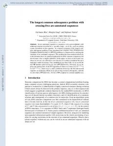
In this section, we present experimental results. We compare the running time of the proposed algorithm in Section 3 to the existing algorithms [2, 15]. Furthermore, we show the running time of Algorithm 2. We used a machine running Ubuntu 14.04 with Core i7 4820K and 64GB RAM. We implemented all algorithms in C++ and compiled with gcc 4.8.4 with -O2 optimization. We used an implementation of the algorithm proposed by Paveti´c et al., available at github.com/fpavetic/lcskpp. We denote the algorithm ˇS ˇ proposed by Paveti´c et al. [15] and the algorithm proposed by Benson et al. [2] as PZ and BLMNS, respectively. ˇ S, ˇ and BLMNS in the following We tested the proposed algorithm in Section 3, PZ three conditions: (1) random strings over an alphabet of size |Σ| = 4 with n = m = 1000, 2000, · · · , 10000 and k = 1, 2, 3, 4 (2) random strings over alphabets of size |Σ| = 1, 2, 4, 8 with n = m = 1000, 2000, · · · , 10000 and k = 3 (3) DNA sequences that are available at www.ncbi.nlm.nih.gov/nuccore/346214858 and www.ncbi.nlm.nih. gov/nuccore/U38845.1, with k = 1, 2, 3, 4, 5. The experimental results under the conditions (1), (2) and (3) are shown in Figs. 3(a), 3(b), and 3(c), respectively. ˇS ˇ for small k or small The proposed algorithm in Section 3 runs faster than PZ ˇ ˇ alphabets. This is due to that PZS strongly depends on the total number of matching k length substring pairs between input strings, and for small k or small alphabets there are many matching pairs. In general BLMNS runs faster than ours. The proposed algorithm runs a little faster for small k or small alphabets, except |Σ| = 1. We think that this is because for small k or small alphabets the probability that L[i, j] ≥ k is high, and this implies that we need more operations to compute M [i, j] by definition. In Fig. 3(b), it is observed that the proposed algorithm with |Σ| = 1 runs faster than with |Σ| = 2. Since |Σ| = 1 implies that X = Y if X and Y have the same length, L[i, j] > k almost always holds, which leads to reduce branch mispredictions and speed up execution. We show the running time of Algorithm 2 in Fig. 3(d). We tested Algorithm 2 on random strings over Σ = {1, 2, · · · , 100} with n = m = 1000, 2000, · · · , 10000 and k = 2, 3, 4, 5. It is observed that the algorithm runs faster as the parameter k is smaller. 10

0.8

1.0 Running Time (sec)

Running Time (sec)

Proposed P BLMNS

k=1 k=2 k=3 k=4

1.0

0.6 0.4 0.2

0.8

|Σ| = 1 |Σ| = 2

|Σ| = 4 |Σ| = 8

Proposed P BLMNS

0.6 0.4 0.2

0.0 0.0 1000 2000 3000 4000 5000 6000 7000 8000 9000 10000 1000 2000 3000 4000 5000 6000 7000 8000 9000 10000 Length Length

(a) Random data; |Σ| = 4; k = 1, 2, 3, 4 3.0

Proposed P BLMNS

2.5

80

2.0

Running Time (sec)

Running Time (sec)

(b) Random data; k = 3; |Σ| = 1, 2, 4, 8 100

1.5 1.0

60 40 20

0.5 0.0

k=2 k=3 k=4 k=5

1

2

3

4

5

k

0 1000 2000 3000 4000 5000 6000 7000 8000 9000 10000 Length

(d) Algorithm 2, random data, |Σ| = 100

(c) DNA data

ˇ S, ˇ and Figure 3: Running times of the proposed algorithm in Section 3, PZ BLMNS (Figs.3(a), 3(b) and 3(c)), and Algorithm 2 (Fig. 3(d)). In Figs. 3(a), 3(b), and 3(c), the line styles denote algorithms. The line markers in Figs. 3(a) and 3(b) represent the parameter k and the alphabet size, respectively. We suppose that the hidden constant of the RMQ data structure described in Section 5 is large. Therefore, the running time of Algorithm 2 depends on the number of times the rmq operation is called, and for small k the number of them increases since the probability that l ≥ k is high.

7

Conclusion

We showed that both the LCSk+ problem and the op-LCSk+ problem can be solved in O(mn) time. Our result on the LCSk+ problem gives a better worst-case running time than previous algorithms [2, 15], while the experimental results showed that the previous algorithms run faster than ours on average. Although the op-LCSk+ problem looks much more challenging than the LCSk+ , since the former cannot be solved by a simple dynamic programming due to the properties of order-isomorphisms, the proposed algorithm achieves the same time complexity as the one for the LCSk+ .

11

Acknowledgements. This work was funded by ImPACT Program of Council for Science, Technology and Innovation (Cabinet Office, Government of Japan), Tohoku University Division for Interdisciplinary Advance Research and Education, and JSPS KAKENHI Grant Numbers JP24106010, JP16H02783, JP26280003.

References [1] M. A. Bender and M. Farach-Colton. The LCA problem revisited. In LATIN 2000, pages 88–94, 2000. [2] G. Benson, A. Levy, S. Maimoni, D. Noifeld, and B. Shalom. LCSk: A refined similarity measure. Theor. Comput. Sci., 638:11–26, 2016. [3] M. Bouvel, D. Rossin, and S. Vialette. Longest common separable pattern among permutations. In CPM 2007, pages 316–327, 2007. [4] S. Cho, J. C. Na, K. Park, and J. S. Sim. A fast algorithm for order-preserving pattern matching. Inf. Process. Lett., 115(2):397–402, 2015. [5] R. Cole and R. Hariharan. Dynamic LCA queries on trees. SIAM J. Comput., 34(4):894–923, 2005. [6] M. Crochemore, C. S. Iliopoulos, T. Kociumaka, M. Kubica, A. Langiu, S. P. Pissis, J. Radoszewski, W. Rytter, and T. Wale´ n. Order-preserving indexing. Theor. Comput. Sci., 638:122–135, 2016. [7] S. Deorowicz and S. Grabowski. Efficient algorithms for the longest common subsequence in k-length substrings. Inf. Process. Lett., 114(11):634–638, 2014. [8] J. Fischer. Inducing the LCP-array. In WADS 2011, pages 374–385, 2011. [9] J. Fischer and V. Heun. Space-efficient preprocessing schemes for range minimum queries on static arrays. SIAM J. Comput., 40(2):465–492, 2011. [10] D. Gusfield. Algorithms on Strings, Trees, and Sequences: Computer Science and Computational Biology. Cambridge University Press, 1997. [11] M. M. Hasan, A. Islam, M. S. Rahman, and M. Rahman. Order preserving pattern matching revisited. Pattern Recogn. Lett., 55:15–21, 2015. [12] R. Khan, M. Ahmad, and M. Zakarya. Longest common subsequence based algorithm for measuring similarity between time series: A new approach. World Appl. Sci. J., 24(9):1192–1198, 2013. [13] J. Kim, P. Eades, R. Fleischer, S.-H. Hong, C. S. Iliopoulos, K. Park, S. J. Puglisi, and T. Tokuyama. Order-preserving matching. Theor. Comput. Sci., 525(13):68–79, 2014.

12

[14] M. Kubica, T. Kulczynski, J. Radoszewski, W. Rytter, and T. Walen. A linear time algorithm for consecutive permutation pattern matching. Inf. Process. Lett., 113(12):430–433, 2013. ˇ zi´c, and M. Siki´ ˇ c. LCSk++: Practical similarity metric for long [15] F. Paveti´c, G. Zuˇ strings. CoRR, abs/1407.2407, 2014. ˇ c, A. Wilm, S. N. Fenlon, S. Chen, and N. Nagarajan. Fast and [16] I. Sovi´c, M. Siki´ sensitive mapping of nanopore sequencing reads with GraphMap. Nat. Commun., 7, 2016.

13