1426
JOURNAL OF PHYSICAL OCEANOGRAPHY
VOLUME 38
Loop Current and Deep Eddies L.-Y. OEY Princeton University, Princeton, New Jersey (Manuscript received 5 April 2007, in final form 15 October 2007) ABSTRACT In contrast to the Loop Current and rings, much less is known about deep eddies (deeper than 1000 m) of the Gulf of Mexico. In this paper, results from a high-resolution numerical model of the Gulf are analyzed to explain their origin and how they excite topographic Rossby waves (TRWs) that disperse energy to the northern slopes of the Gulf. It is shown that north of Campeche Bank is a fertile ground for the growth of deep cyclones by baroclinic instability of the Loop Current. The cyclones have horizontal (vertical) scales of about 100 km (1000⬃2000 m) and swirl speeds ⬃0.3 m s⫺1. The subsequent development of these cyclones consists of two modes, A and B. Mode-A cyclones evolve into the relatively well-known frontal eddies that propagate around the Loop Current. Mode-A cyclone can amplify off the west Florida slope and cause the Loop Current to develop a “neck” that sometimes leads to shedding of a ring; this process is shown to be the Loop Current’s dominant mode of upper-to-deep variability. Mode-B cyclones are “shed” and propagate west-northwestward at speeds of about 2–6 km day⫺1, often in concert with an expanding loop or a migrating ring. TRWs are produced through wave–eddy coupling originating primarily from the cyclone birthplace as well as from the mode-B cyclones, and second, but for longer periods of 20⬃30 days only, also from the mode-A frontal eddies. The waves are “channeled” onto the northern slope by a deep ridge located over the lower slope. For very short periods (ⱗ10 days), the forcing is a short distance to the south, which suggests that the TRWs are locally forced by features that have intruded upslope and that most likely have accompanied the Loop Current or a ring.
1. Introduction The Loop Current and warm-core rings, which episodically separate from the Loop Current, are powerful features that dominate the upper (surface to depths of 500⬃1000 m) circulation in the Gulf of Mexico. A recent book (edited by Sturges and Lugo-Fernandez 2005) provides a glimpse of the vast knowledge that has accumulated in the past decades. The Loop Current and rings are well studied because they are so prominently important, of course; they are also very obvious manifestations of the system, being more readily observable, especially in recent decades thanks to satellite data. The Loop Current and rings affect, either directly or indirectly through their smaller-scale subsidiaries, just about every aspect of oceanography in the Gulf of Mexico. One such aspect concerns deep eddies that are much less accessible, hence less known and understood. In recent years, deep eddies and circulations in general
Corresponding author address: L.-Y. Oey, 14 Taunton Court, Princeton Junction, NJ 08550. E-mail:
[email protected] DOI: 10.1175/2007JPO3818.1 © 2008 American Meteorological Society
have received increased attention, in part because of practical needs spurred by oil and gas activities in deeper waters of the gulf. Indeed, the abundance of deep eddies, cyclones in particular, has been recently noted in observations (A. Lugo-Fernandez, 2007, personal communication). Here, by “deep” I mean 1000 m and deeper. At these depths, the gulf is virtually closed except for the deep, narrow opening at the Yucatan Channel. The Loop Current and rings are therefore the major source of energy for deep eddies, which are generated and dissipated within the Gulf. They provide mixing below the thermocline and may play a crucial role in the overall energy balance, which in turn may affect the Loop Current and its behaviors, including the separation of rings. As will be seen, deep eddies are generally vertically coherent (cf. Welsh and Inoue 2000), with scales of 1000⬃2000 m: from approximately 1000 m below the surface to the bottom (above the bottom boundary layer); therefore, they tend to be effective in producing cross-isobath motions, hence possibly also topographic Rossby waves (TRWs). Pioneering deep observations consist of hydrographic measurements, primarily by
JULY 2008
OEY
1427
FIG. 1. A locator map of the study region. The whole domain shown is the parent model domain. Time-independent inflow and outflow that account for the large-scale transports (Svedrup ⫹ thermohaline) are specified across the open boundary at 55°W as a function of latitude. Contours show isobaths in m. Dashed lines enclose the nested double-resolution Gulf of Mexico domain.
oceanographers from Texas A&M University in the 1950s and 1960s (see summaries in the book edited by Capurro and Reid 1972). The first published report of direct current observations in the deep gulf appears to be Hamilton (1990),1 who found that subinertial deep currents over the lower continental slope (depths ⬃3000 m) were dominated by motions having the characteristics of TRWs with periods ⱗ100 days and trapped over depths ⬃1000 m from the bottom. Given the bowl-shape topography of the Gulf of Mexico, the dominance of TRWs in deep layers of the gulf is, in retrospect, not surprising. More recently, Hamilton and Lugo-Fernandez (2001) and Hamilton (2007) observed energetic deep currents at the Sigsbee Escarpment (hereafter termed only Sigsbee; marked by a cross in Fig. 1)—a steep undersea cliff with vertical drops of approximately 500 m (10 km)⫺1 near the 2000-m isobath in the north-central Gulf of Mexico (Fig. 1); the escarpment separates gentler topographies north and south. The deep currents again have the characteristics
1
Maul et al.’s (1985) observations were earlier, but were made in the deep layers of the Yucatan Channel.
of TRWs, but with shorter periods of 5–30 days. The authors found that the energy decreases rapidly, within O(10 km), northward across the escarpment. In addition to the possibility of localized (direct) forcing, due to, say, the Loop Current or a powerful ring over the continental slope, TRW energy propagation triggered remotely by mesoscale variability, also from the Loop Current or rings, has been proposed as a viable generation mechanism (e.g., Oey and Lee 2002; hereafter OL02; Hamilton, 2007). However, the ideas have never been fully elucidated. In this paper, we attempt to explain the origin and nature of the remote forcing by way of numerical modeling and analyses. It will become obvious that deep eddies play an important role in forcing the TRWs. Oey and Lee (2002) also analyzed TRWs in the Gulf by means of numerical modeling and ray tracing. However, they focused on TRW periods ⬎30 days and showed significant deep energy in the vicinity of the 3000-m isobath in the central gulf, but not to the north near the escarpment at the 2000-m isobath; their conclusions are not inconsistent with Hamilton’s (2007) findings. Oey and Lee (2002) also suggested a higher grid resolution to resolve the step topography of the
1428
JOURNAL OF PHYSICAL OCEANOGRAPHY
escarpment. In this work, the resolution of Oey and Lee’s model is doubled. By using a model to infer circulation physics, we implicitly presume that the model, while it is never perfect, can at least capture some features of the Loop Current dynamics including the shedding of rings. Oey et al. (2005a) review Gulf of Mexico models that are presently in use. Most of these, including ours, appear to be quite capable of reproducing some gross features of the Loop Current and rings, such as the transports, maximum speeds, and eddy-shedding rates. Section 2 describes the model, section 3 contains the main results, and section 4 summarizes the paper.
2. The model The Princeton Regional Ocean Forecast System (PROFS) model, used here (see http://www.aos. princeton.edu/WWWPUBLIC/PROFS/ for publications pertaining to the testing, process studies, skill assessment, and other appications of PROFS), is based on the Princeton Ocean Model (POM; see Mellor 2004). The model results have been compared with observations including in situ and shipboard ADCP data (Wang et al. 2003; Oey et al. 2005a,b; Lin et al. 2007; Yin and Oey 2007), drifters and satellite data (Fan et al. 2004; Lin et al. 2007; Yin and Oey 2007), flows in the Yucatan Channel (Ezer et al. 2003; Oey et al. 2004, 2005a), and National Data Buoy Center (NDBC) data (Oey et al. 2006, 2007). Here, only those model features pertinent to the present study are described. The model consists of a parent model and a nested model as shown in Fig. 1. The parent model has the same domain, resolution, and forcing as those described in our previous works (e.g., Oey et al. 2003). Thus, the parent model’s horizontal grid size is approximately 10 km in the Loop Current and northwestern Caribbean Sea and about 5 km in the northeastern Gulf of Mexico. There are 25 terrain-following (the so-called sigma coordinate) levels. At water depths of about 2500 m, the vertical grid sizes are about 10 m near the surface and bottom but coarser, around 210 m, for midwater depth. The middepth grid size of 210 m, while not ideal, should be adequate to resolve deep coherent scales O(1000 m). Open boundary conditions at 55°W are specified as in Oey and Chen (1992a). The nested model will be used in all of the analyses presented here; it has a domain focusing on the Gulf of Mexico, a portion of the northwestern Caribbean Sea, and the U.S southeastern shelf and slope; its outer boundary coincides with a parent model’s grid line specified by the user, as indicated in Fig. 1. The horizontal grid sizes are exactly half of those
VOLUME 38
used for the parent grid; thus, four fine grid cells are exactly contained within one parent grid cell, and ⌬x and ⌬y are ⬃5 km in the Loop Current and 2⬃3 km near the Sigsbee Escarpment. The same vertical resolution and physics are used as in the parent grid. The nesting technique is flux conserving (Oey and Chen 1992b) except that in the present case one-way nesting is employed: the nested domain receives boundary information from the parent model, but there is no feedback from the fine grid to the parent grid. This same one-way nested-grid model was used in Oey and Lee (2002) to simulate the generation of long-period TRWs (⬃60 days) as the Loop Current vacillates across the 3000-m isobath. Oey and Zhang (2004) also used the same model to suggest that subsurface jets in the northern gulf, which have been observed, are produced by the interaction of the Loop Current or rings with the continental slope. The parent grid was initialized from a previous 16-yr run with climatological forcing (experiment B of Oey et al. 2003) and continued for another 11 years, which in the model outputs are dated from 1992 through 2002 (the dates are for convenience only and otherwise have no significance).2 The nested grid was run for the same period. Most of the statistics presented herein are based on the 1993–2002 results (10 yr); shorter 3-yr periods, 1993–95, are then used to explain specific ideas. The 10-yr data are adequate to study deep processes (eddies and TRWs) with time scales of around 200 days and shorter.
3. Results I first use empirical orthogonal function (EOF) analyses to connect deep circulation with Loop Current variability, including ring shedding. Propagating deep cyclones are shown next; their connections with and effects on the regional current variability are interpreted using complex EOFs. Topographic Rossby wave energy paths or rays are then computed to help establish the link between deep cyclones and energy over the upper slope near the Sigsbee Escarpment. Idealized model theory is then used to describe how propagating deep cyclones excite TRWs. Finally, current energetics are analyzed, which indicate the dominance of baroclinic instability as the cause for deep cyclogenesis north of Campeche Bank.
2 The model uses dates to keep track of time; dates are also used for ongoing comparison with various other, more complicated model experiments that have winds and data assimilations.
JULY 2008
1429
OEY
a. Surface and deep variability Major features of the modeled circulation in the upper layers (surface to depths 500⬃1000 m), including the Loop Current’s south–north vacillations, ring shedding, and propagation of rings, are similar to those reported in previous works (e.g., Oey et al. 2003) and are not repeated here. At z ⬇ ⫺900 m, observational analysis of the (profiling) autonomous Lagrangian circulation explorer (PALACE) floats suggests a cyclonic gyre west of approximately 90°W (Weatherly et al. 2005; see also the review in Oey et al. 2005a). This large-scale “mean” circulation exists also in the 10-yr-averaged currents of the present model (cf. OL02). On the other hand, deep motions (below z ⬇ ⫺1000 m) with scales of 150 km and less at the high resolution simulated here have not been previously discussed. We first examine how surface and deep variability are related; this is a topic of interest since the deep circulation drives TRWs. Spatial patterns are inferred using EOF analyses on the relative vorticity stretching term PV2 ⫽ (/z)/o at z ⫽ ⫺250 m (near the surface) and in the deep level at z ⫽ ⫺1550 m (Fig. 2).3 The PV2 is the dominant varying term of the Ertel potential vorticity and is a useful indicator of deep eddies (cf. Candela et al. 2002; Oey 2004). Owing to the huge amount of data involved, the EOF is computed only in the northeastern Gulf, and the PV2 is subsampled from smoothed 5-day running averages. The 5-day averaging also reduces noise, especially in deep layers. The analysis is for 10 years, of which a 3-yr time series is shown in Figs. 2a,b. North et al.’s (1982) estimates for EOF degeneracy were computed, indicating good modal separation for surface modes 1 and 2, but only barely so for the deep modes. Figure 2b shows that the surface modes 1 and 2 are in quadrature. Together they contain 50% of the total variance. Figures 2b–d indicate that they represent east–west and south–north expansion and retraction of the Loop Current, as well as shedding and westward propagation of rings, time scales being 6⬃12 months (Fig. 2b) (cf. Oey 1996; Oey et al. 2003). These features (Loop Current’s expansion and retraction and shedding of rings) are readily verified by reconstructing PV2 maps using only modes 1 and 2, as well as by a complex EOF analysis (Horel 1984; Merrifield and Guza 1990), which yields the phase propagation (both not shown). Higher surface modes (3; not shown) represent smaller-
scale features with shorter time scales of 2⬃3 months; these higher modes are not relevant for the present discussion.
DEEP
The subscript 2 in PV2 follows the notation used in Oey (2004), in which PV1 was used for contribution from the planetary vorticity f.
LOOP CURRENT
RETRACTION, AND
The first two deep modes account for only 34% of the total variance. This suggests nonnegligible contributions from higher modes, as we will see with the complex EOF analysis. Nonetheless, understanding the two leading modes is sufficient for the purpose of relating the upper- and deep-layer variability in the Loop Current. Figure 2e shows that the deep EOF mode-1 eigenvector (at z ⫽ ⫺1550 m) has a tripolar structure (negative, positive, and negative) along a southwest– northeast line from Campeche Bank to the west Florida slope.4 Southward along the west Florida slope, a weaker positive pole can also be seen. A tripole is also seen in the deep mode-2 eigenvector (Fig. 2f), but along the west Florida slope the paired “negative–positive pole” of mode 1 switches signs in mode 2. The sign switch makes the line joining the tripole in mode 2 more west–east oriented rather than northeast, and there is a more extensive center “positive pole,” which would reflect the variability under the Loop Current (see below), as well as a negative band around the northern edge of this center pole. The similarities of these deep tripole structures in modes 1 and 2 in the vicinity of the Loop Current suggest that both modes contribute to deep variability under the Loop Current since they would then vary approximately in concert. We see from Fig. 2a that deep mode-1 EOF (at z ⫽ ⫺1550 m) is correlated with and leads the surface mode-1 EOF (C ⫽ 0.7 at 35 days, where C is a crosscorrelation coefficient). Moreover, though not shown here, deep modes 1 and 2 are approximately in phase (mode 1 leads mode 2 by about 10 days); the time series of the sum of deep modes 1 and 2 is therefore also significantly correlated with and leads the surface mode-1 EOF (C ⫽ 0.73 at 20 days). One can better understand how the deep tripole relates to the surface circulation through an example of a ring-shedding event (Fig. 3), with maps reconstructed from the sum of deep modes 1 and 2, referred to as DM1⫹2 (Fig. 4). In Fig. 3, Eulerian trajectories at z ⫽ ⫺1550 m are colored with the local /f and the panels are sequenced at a
4
3
TRIPOLE,
EDDY SHEDDING
In the vicinity of the Loop Current, there is also a small negative pole just shoreward of the 3000-m isobath at 87°W, 26.5°N. This pole is a manifestation of frontal eddies that develop around the northern edge of the Loop Current.
1430
JOURNAL OF PHYSICAL OCEANOGRAPHY
VOLUME 38
FIG. 2. EOF modes 1 and 2 of the relative vorticity stretching term PV2 ⫽ (/z)/o at (a)–(d) z ⫽ ⫺250 m and at (e), (f) z ⫽ ⫺1550 m. (a), (b) Time series from 1993 to 1995, and (c), (d) the corresponding eigenvectors (shaded is negative). In (a), time series of mode-1 EOF at z ⫽ ⫺1550 m is also shown (light line), and in (b), the mode-1 time series at z ⫽ ⫺250 m [from (a)] is superimposed on mode 2 (light line) to show that modes 1 and 2 are in quadrature (1 leads 2). (e), (f) Modes 1 and 2 eigenvectors at z ⫽ ⫺1550 m. (c)–(f) Dashed lines indicate the 200-, 2000-, 3000-, and 3500-m isobaths.
10-day interval; contours of sea surface height (SSH) are also superimposed to indicate the position of the Loop Current and rings. In Fig. 3a, the Loop Current is in an extended state. Figures 3b,c show that a cyclone at the northeastern edge of the Loop Current propagates southward along the west Florida slope, amplifies (Figs. 3d,e; cf. observations by Fratantoni et al. 1998), and then cleaves the Loop Current, which then develops a “necking” (a term used by Schmitz 2005; Fig. 3f); the amplified cyclone appears to have caused a ring to detach from the Loop Current (Figs. 3g,h; see the cyclone near 25°N, 85.5°W). The Loop Current then reforms, and a deep anticyclone forms near where the cyclone previously was (Figs. 3i–l). Figure 4 illustrates how deep modes 1 and 2 account
for the dominant signal of the above scenario. Figures 4a–d show the tripole formation, which is most noticeable by the intense negative pole off west Florida. The subsequent southwestward penetration of the cyclone and Loop Current cleaving (e.g., Figs. 3e–h) is seen as a reversal in the sign of the tripole: negative at the center and positive on both sides (Figs. 4e–h). In Figs. 4i–l, the tripole begins to lose its signature as the center pole changes sign (again) and mode 2 dominates (because the mode-1 temporal EOF is ⬃0); this is when the Loop Current reforms and the deep anticyclone appears surrounded by deep frontal cyclones (Figs. 3k,l), which can be seen in deep mode 2 (Fig. 2f). In Figs. 4i–l, as the ring moves westward, a comparison with Fig. 2f shows that the response is mostly contributed by mode
JULY 2008
OEY
1431
FIG. 3. Maps of deep flows (z ⫽ ⫺1550 m) indicated by 30-day Eulerian trajectories x ⫽ xo ⫹ 兰u dt, where x and u are position and velocity vectors, respectively; the integration is over 30 days. The trajectories are launched from every eighth grid point. Colors indicate the local values of the relative vorticity /f (blue is cyclonic and red anticyclonic). Thick contours are the SSH (0, 0.25, and 0.5 m). Maps are shown every 10 days for a total of 120 days, during which a ring is shed. Gray contours are isobaths (200, 2000, 3000, and 3500 m), and the red plus sign identifies the Sigsbee location.
2, especially in the western and northern regions of the domain shown. The above behavior of DM1⫹2 and its connection with the Loop Current are robust. The generality of the results is seen in the temporal EOFs (e.g., Figs. 2a,b), which indicates near-periodic oscillations with period ⬃10 months. In terms of the surface EOFs (z ⫽ ⫺250 m), the Loop Current necking is represented by the (positive) peaks in the temporal mode-1 EOF (dark line in Fig. 2a) combined with the negative spatial mode 1 over the Loop Current in Fig. 2c (the result is a PV2 ⬍ 0 cyclone; the example shown in Fig. 3e,f corresponds to the first peak). Since deep (z ⫽ ⫺1550 m)
EOFs lead the surface, the surface peaks are preceded by deep peaks (Fig. 2a) that correspond to the strengthening of the deep tripole, the west Florida pole (PV2 ⬍ 0, cyclone in Fig. 2e) in particular; also, as the deep EOFs switch sign to become negative, the cyclone penetrates under the Loop Current (PV2 ⬍ 0; Figs. 2a,e). Subsequent Loop Current reformation (Figs. 3j–l, 4j–l) near the Yucatan Channel (PV2 ⬎ 0, anticyclone) is relatively rapid (weeks) as the surface temporal mode 1 passes through zero to become negative, but the deep EOFs yet again switch sign to positive (Fig. 2a). The necking-down process sometimes leads to ring shedding, but not always. That the deep modes (1 and 2)
1432
JOURNAL OF PHYSICAL OCEANOGRAPHY
VOLUME 38
FIG. 4. Maps of reconstructed EOF modes 1 and 2 at z ⫽ ⫺1550 m of the relative vorticity stretching term PV2 ⫽ (/z)/.
lead the corresponding surface modes, as mentioned above, and the time scale is 30⬃40 days for the deep tripole to change sign when necking occurs (Figs. 2a and 4c–f) strongly suggests a process dominated by baroclinic instability; this is not a new finding (e.g., Hurlburt and Thompson 1980). What is new is our demonstration that, in the model, the process is a dominant mode of eddy variability in the eastern gulf that links both surface and deep circulations and that the amplification of propagating frontal eddies along the west Florida slope plays an important role in the process. This link was suggested by Schmitz (2005) based on satellite images. However, in the model, the neck-
ing-down process is initiated primarily by the west Florida pole. The Campeche Bank pole of the above tripole is a response similar to what Schmitz (2005) referred to as the Campeche Bank “Cyclonic Eddy,” and the west Florida pole is his West Florida Cyclonic Eddy. Schmitz’s descriptions are primarily based on objective analyses of satellite SSH anomalies and sea surface temperature; he focuses on the necking-down scenario and its connection with the shedding of rings as well as on the propagation of frontal eddies around the Loop Current. In this regard, the model analysis supports his inferences. However, as will be shown, the model’s
JULY 2008
OEY
1433
FIG. 5. Monthly examples of deep cyclones, labeled A and B, being forced westward by an expanding Loop Current. Trajectories at z ⫽ ⫺1550 m are plotted as in Fig. 3, and swirl speeds (m s⫺1) at some representative positions marked by an asterisk are printed. Black contours are SSH ⫽ 0.1, 0.3, and 0.5 m. In addition to eddies A and B, other cyclones are also identified in gray letters (see text). Gray contours are isobaths (200, 2000, 3000, and 3500 m), and the red plus sign identifies the Sigsbee location.
Campeche Bank pole is dominantly related to the development of deep cyclones, which are most effective in generating TRWs.
b. Propagating deep cyclones and their consequences Before examining coherent patterns from complex EOFs for the 10-yr model results, a phenomenological description of deep eddies is first given, using Figs. 3 and 5 as examples, to indicate the eddy types, scales, and intensities. Figure 3 shows deep eddies with scales from about 50 to 150 km. Apart from the larger deep cyclone that develops under the Loop Current, which is tending to pinch off, smaller eddies (dominated by cyclones) are ubiquitous and are prevalent through the 10-yr simulation (e.g., http://aos.princeton.edu/ WWWPUBLIC/PROFS/animations.html). Cyclones
appear as Loop Current frontal eddies (e.g., Fratantoni et al. 1998) that are more confined to the upper layer (0⬃1500 m) or as deep columnar features that are vertically coherent from approximately 1000 m below the surface to the top of the bottom boundary layer (not shown here, but see the aforementioned Web site or OL02’s vector stick plots, their Fig. 14). Long-term currents collected at (25.5°N, 87°W; water depth ⬃3300 m) show good vector correlation from 1200 m below the surface to 150 m above the bottom (M. Inoue, 2006, personal communication). Welsh and Inoue (2000) reported deep eddies through the narrow opening (seen in the converging 3000-m isobaths around 88°W) that connects the deep eastern and western basins of the Gulf. In the present analysis, migrating deep eddies are seen in the maps for deep modes 1 and 2; in particular, Figs. 4i–l show coherent features westward from north
1434
JOURNAL OF PHYSICAL OCEANOGRAPHY
of the Campeche Bank; these features are forced by the westward-migrating ring (Figs. 3i–l). Deep eddies can also be forced to propagate westward by an expanding Loop Current; an example is given in Fig. 5. Cyclones A and B both originate north of Campeche Bank and move westward ahead of the northwestward-extending Loop Current; the cyclone swirl speeds are 0.2⬃0.3 m s⫺1 (selected speeds are printed in Fig. 5). The weaker cyclone “B1” actually was split off from eddy “B” at an earlier time, while eddy “C” was spun off from the small surface warm ring located over the slope (Fig. 5a). As the Loop Current extends over the slope near Sigsbee (marked by a red plus sign), a small cyclone “S” is produced (Figs. 5b–d; cf. Oey and Zhang 2004). These (and other) deep eddies move in a complicated fashion because of nonlinear vortex interactions, though the net propagation is westward. Despite their complicated movements, Fig. 5 shows that some of these cyclones are surprisingly resilient: they can persist for months. Cyclones can also spontaneously grow (in a few days); a good location for cyclogenesis is north of the Campeche Bank. In Figs. 5c,d, for example, cyclone “D” can be seen to develop.
1) COMPLEX EOF Complex EOF (CEOF) is used to analyze deep eddy patterns that can involve propagation. Apart from directly forced modes (e.g., Fig. 5), propagating features that are not in unison with either the Loop Current or rings are also of interest. In CEOF (Horel 1984; Merrifield and Guza 1990), we construct the covariance matrix from complex time series (for each grid point) that are a sum of the original series plus an imaginary part that is the Hilbert transform of the original series. The resulting CEOF has, for each CEOF mode n, complex temporal expansion An(t) and eigenvector Bn(x) (x the position vector), which therefore have amplitudes as well as phases: | An| and n as functions of time t and |Bn| and n as functions of x. Plots of n and n provide propagation information; in fact, for each CEOF mode, the phase velocity is cn ⫽ 共dnⲐdt兲Ⲑ共n兲.
共1兲
We apply CEOF to PV2 ⫽ (/z)/o. To focus on patterns west of the Loop Current, we reduce the influences of the west Florida pole (discussed above) by choosing a smaller domain west of 86°W (instead of west of 84°W used in Fig. 2).5 The resulting surface
VOLUME 38
CEOF modes do not provide any additional insight than what was previously discussed in conjunction with Fig. 2; thus, we focus on only the deep CEOF modes at z ⫽ ⫺1550 m. The CEOF analysis was conducted for the entire 10 years. For clarity in showing short periods (months) in the temporal modal structures, 3-yr time series are displayed in Fig. 6 (as in Figs. 2a,b); these are typical of the rest of the time series (not shown). Figure 6 shows the temporal amplitude |An|, phase n, and spectra of Re(An) ⫽ |An| cosn6 for the three leading CEOF modes 1, 2, and 3, and Fig. 7 gives the corresponding spatial (i.e., from the 10-yr analysis) amplitudes |Bn| (normalized), phases n, and reconstructed maps represented by |Bn| (cosn ⫹ sinn). The corresponding long-time (10 yr) mean SSH contours (0.15 and 0.35 m) are also plotted in Fig. 7 to indicate the mean position of the Loop Current in relation to the modal structures. A few explanations on the CEOFs are warranted. First, the percentile variances of the three CEOF modes (20:16:12; printed in the figures) and the separation of their eigenvalues are relatively small. Deep eddies are highly chaotic, and understanding patterns of variability (e.g., using EOFs), as discussed below, should preferably be guided by plausible physical reasoning as well as by evidence derived from other independent methods (described below). Second, the time-varying portion of each CEOF mode is represented by a combination of both the modal amplitudes and phases, not by each one individually; we therefore plot the spectra of Re(An) in Fig. 6. Third, the temporal phases (Fig. 6, middle) are in general increasing CEOF mode 1 more uniformly (slope ⬇ 2/200 days) than the other two modes. Moreover, mode 1 has a strong, nearly periodic 200-day component related to the expansion and retraction of the Loop Current, including ring shedding (see Fig. 2); this component is therefore removed when plotting mode-1 spectra in Fig. 6 so that the variance at shorter periods may be compared with the other two modes. Fourth, because of the generally increasing temporal phases (Fig. 6, middle), the direction of phase propagation (at an x location) is generally in the direction of increasing (spatial) phase, as schematically shown by the vectors in Fig. 7 (middle). Finally, the reconstructed spatial structures (Fig. 7, right) are only representative, as equal weights are given to cosn and sinn. Unlike the amplitude maps, which are wholly positive (Fig. 7, left), the reconstructed maps do give some idea of the relative positions of eddies for
5
This precautionary step, however, turns out to be unnecessary, and the results for regions to the west of the Loop Current are very similar to those obtained below if the west Florida pole is also included.
6 Actual fluctuations at any x contain other terms and multiples, but spectral level and distribution are well-represented by |An| cosn.
JULY 2008
OEY
1435
FIG. 6. (left) Time series of amplitudes and (middle) phases of CEOF (top to bottom) modes 1, 2, and 3, and (right column; note change of scale for mode 1) their respective spectra.
each mode; they should, however, be interpreted in conjunction with the amplitude maps.
2) INTERPRETING
THE
CEOF
MODES
The CEOF mode 1 has a pair of poles near 25.5°N, 88°W (Figs. 7a,c) consisting of two oppositely signed eddies on either side of the Loop Current’s mean outer edge, taken to be SSH ⫽ 0.15 m (cf. Leben 2005, who used 0.17 m as the outer edge). The larger southern pole, which is negative or cyclonic, is located north of Campeche Bank and is also seen in modes 2 and 3, though varying in position and size; it is caused by frequent amplification of (small-scale perturbations into)
deep cyclones exemplified by cyclones “A,” “B,” and “D” of Fig. 5, described previously [hereafter, these eddies will be called the North Campeche Bank Cyclones (NCBCs)]. As will become clear, baroclinic instability is responsible for the amplification of the NCBCs into deep cyclones. The amplification is brought about as the Loop Current flows over the Campeche Bank into the deeper gulf. However, apart from this common cause, the three modal patterns represent different physical processes. For CEOF mode 1, the positive (northern) pole of the paired pole is, in fact, near where OL02 previously identified a “trigger point” of westward-propagating long-period TRWs
1436
JOURNAL OF PHYSICAL OCEANOGRAPHY
VOLUME 38
FIG. 7. (left) Maps of spatial amplitudes and (middle) phases of CEOF (top to bottom) modes 1, 2, and 3, and (right; see text) their reconstructions. (a)–(i) The Sigsbee location is marked with a plus sign, and on (i), the two other locations where energy spectra are shown in Fig. 8 are also marked. Thick gray lines show the 0.15- and 0.35-m contours of the 10-yr model mean SSH, indicative of the mean position of the Loop Current. Thin contours show isobaths: 200, 2000, 3000, and 3500 m. Dark arrows indicate TRW ray sites, and white arrows indicate sites of deep eddies, discussed in the text.
(60⬃100 days) along the 3000-m isobath (it is the origin of OL02’s ray 2; see their Figs. 11, 13).7 OL02 show that these waves tend to converge around 90°W (on the 3000-m isobath; see OL02’s Fig. 11a), a location that agrees well with the location of the third (westernmost) dominant pole of CEOF mode 1, seen in Fig. 7a. The existence of these long-period TRWs in the present simulation is readily verified by repeating the OL02 7 The waves are a mix of topographic and planetary Rossby waves; the ratio of topographic to planetary beta, f |h|/(h), is about 5 (see OL02’s Fig. 11b).
analysis (results are not shown here). Suffice to say that, in addition to the 60⬃100-day waves, longer periods (about 140 days) are also found (see spectra in Fig. 6c; note that the spectra show very weak variances for periods shorter than 80⬃100 days). The waves are also confirmed by the offshore-directed phase propagation (dark arrows in Fig. 7, middle), which therefore indicates energy propagation at approximately /2 clockwise, or generally westward in the direction of the isobath (see, e.g., OL02). Moreover, the Loop Current’s presence in CEOF mode 1 (in addition to the nearly constant temporal phase noted previously, Fig. 6b) is
JULY 2008
OEY
also seen in Figs. 7a,c as a relatively large spatial amplitude region under the Loop Current (but weaker than the other three CEOF-mode1 poles mentioned above). These and the OL02 results strongly suggest that the three coherent poles of CEOF mode 1 represent responses of long-period TRWs triggered by oscillatory movements of the Loop Current (including ring shedding); the western edge of the Loop Current, around 25.5°N, 88°W in the model, appears to be a site where triggering occurs. To the best of my knowledge, this is the first time that the link among the Loop Current, deep eddies, and TRWs has been identified, though OL02 did describe one example of the phenomenon (see their Fig. 18). Note that in Figs. 7a,c (also in the corresponding amplitude maps for CEOF modes 2 and 3, Figs. 7d,f,g,i), there is only a weak coherent pattern that relates TRWs west of 88°W with eastwardpropagating frontal eddies around the northern edge of the Loop Current (white dotted arrows in Fig. 7b); these east-northeastward propagating frontal eddies will be referred to as mode-A eddies or cyclones; they are also evident from the EOF mode 2 discussed previously (Fig. 2f). Oey and Lee (2002) suggested that the mechanism for the generation of these TRWs is similar to that invoked by Pickart (1995) for TRWs produced by Gulf Stream meanders off Cape Hatteras. Although the existence of the OL02 trigger point, mentioned above, is now confirmed, the authors appear to have overstated the role of the mechanism in the case of Loop Current frontal eddies. But, why is it that, near the location of the northern pole of the aforementioned paired pole (i.e., near OL02’s trigger point), northwestward-propagating perturbations along the inflowing Loop Current can trigger energetic TRWs? This question will be addressed later. Of the three CEOF modes, and for periods shorter than approximately 150 days, CEOF mode 2 contains the largest variance (Fig. 6f). The spatial amplitude map (Fig. 7d) again shows large values north of Campeche Bank. As with CEOF mode 1, the mode-2 temporal phase (Fig. 6e) generally increases but it also shows more frequent reversals, suggesting stalled eddies. Thus, together with spatial phase and reconstructed maps (Figs. 7e,f), CEOF mode 2 represents deep eddies that propagate west-northwestward, often synchronously with the expanding Loop Current and rings (e.g., Fig. 5), and the phase reversals represent forcing by the Loop Current variability (e.g., retractions) and also by rings that can stall within the analysis region. The relatively large spectral variance around 150 days, in Fig. 6f, indicates the influence of the Loop Current and rings. Figure 6f also shows peaks at periods
1437
around 80 and 30 days, suggestive of TRWs, which are indicated along approximately the 3000-m isobath by the corresponding spatial maps (Figs. 7e,f). The CEOF mode 3 (Figs. 7g–i) is conspicuously characterized by its significant spatial amplitude (Fig. 7g) that spans almost the entire width of the continental rise, bounded by the 3000 (north) and 3500-m (south) isobaths, and zonally over a distance of almost 300 km from 87.3° to 90°W. The spatial phase indicates a westward translation of deep features (depicted by the long arrow in Fig. 7h). The temporal phase is generally increasing (Fig. 6h). Although the frequency is relatively high (dn/dt is large), so is its wavenumber (⫺n/x) in the aforementioned region of significant spatial amplitude. The first-mode baroclinic planetary wave speed (westward, same as below) is ⬇R2o /2 ⬇ 0.5–1 km day⫺1 for wavelengths of about 2Ro ⬇ 100–150 km, assuming a Rossby radius Ro of about 20–30 km (Chelton et al. 1998; Oey et al. 2005a). The actual eddy’s propagation phase speeds from Figs. 6h and 7h (or approximately from tracking actual features, e.g., Fig. 3, or more exactly from reconstructed mode-3 maps, not shown) are about 2–6 km day⫺1. As noted previously, since the deep features are vertically coherent from approximately 1000 m below the surface to near the bottom, the effects of topography cannot be ignored and the higher speeds are explained in terms of Rossbywave propagation on the topographic beta (T) plane, where T ⫽ f |h|/(h) ⬇ 5. In contrast to the deep features seen in CEOF mode 2, the CEOF mode 3 represents purely westward-propagating eddies that are not necessarily in unison with the Loop Current expansion or with migrating rings. This is evidenced by the lack of energy at long periods ⬃200 days (Fig. 6i). In other words, in CEOF mode 3, once the NCBC is formed, it “escapes” westward. Examples are the cyclone labeled B in Fig. 5, as well as similar eddies (of both signs) seen in Figs. 3a–f. I will refer to these west-northwestward propagating deep eddies as mode-B eddies or cyclones, in contrast to the mode-A Loop Current frontal eddies, regardless of whether they are CEOF modes 1, 2, or 3. An interesting consequence of these mode-B eddies with an along-isobath propagating component over the lower continental slope is that they are efficient exciters of onslope (i.e., north-northwestward) propagating TRWs (see below). Figure 8 shows energy spectra at three stations along a ray path suggested by the mode-3 phase map (Figs. 7h,i): at a source location north of the westward-propagating eddies over the lower continental slope (right), at the Sigsbee Escarpment (left), and at a location in between over the midslope (middle). These
1438
JOURNAL OF PHYSICAL OCEANOGRAPHY
VOLUME 38
FIG. 8. Energy spectra at three indicated stations: (right) lower continental slope, (left) the Sigsbee Escarpment, and (middle) over the midslope. For each location, spectra at three depths are plotted: (top) 200 m below the surface, (middle) middepth, and (bottom) 200 m above the bottom. Both the west–east (u, dotted line) and south–north (, dashed line) components are plotted as well as their sum (solid line).
were computed based on 1993–95, 5-day-averaged results. For each location, spectra at three depths are plotted at 200 m below the surface, at middepth, and at 200 m above the bottom. Both the west–east (u: dotted line) and south–north (: dashed line) components are plotted as well as their sum (solid line). Figure 8 shows a number of notable features. First, energy near the escarpment (Sigsbee: note change of the y scale in Fig. 8 for this location; left column) is, in general, smaller than those over the middle and lower slopes at all three depths. Second, near the surface, there is a broad spectral peak centered near 200 days at all three locations, indicative of strong influence from the Loop Current vacillations as well as from rings. The strong Loop Cur-
rent and ring presence at Sigsbee has been observed (Hamilton and Lugo-Fernandez 2001; Lai and Huang 2005; Hamilton 2007; Lin et al. 2007). The surface energy at the lower-slope location (Fig. 8, right column) is slightly smaller than that at midslope (Fig. 8, middle column) where there is additionally a much stronger peak near 100 days. This is because the midslope position is directly in the path of the Loop Current fluctuations and ring shedding, whereas the lower-slope location is sheltered at the southwestern corner of the Loop Current path. Third, contrary to the surface spectra, stronger middepth energy is seen at the lower slope than at midslope, particularly at periods shorter than about 50 days (Fig. 8, middle row). Thus, as seen in the
JULY 2008
OEY
1439
CEOF’s spatial structures (Figs. 7a,d,g), deep energetic eddies are developed (in the model) north of Campeche Bank. Finally, energy intensification can be seen from middepth to the bottom, especially at the Sigsbee and midslope locations, for periods shorter than 100 days (Fig. 8, lower-left four panels). At Sigsbee (Fig. 8, left column), energy intensification occurs at periods shorter than 30 days, in agreement with Hamilton’s (2007) observations. At the “source” location over the lower slope, the spectra changes from being broad at middepth to bottom intensified at selected periods near 30 and 20 days (Fig. 8, right column’s second and third panels). Note also that the component energies change from predominantly north/ south () near the surface to along isobaths (u for Sigsbee and lower slope, and 45° to north at midslope) near the bottom. These features are all characteristic of TRWs (e.g., OL02).
c. Deep energy paths–TRW rays There are, therefore, primarily three ways in which TRWs found over the slope may be excited by deep eddies to the south and east, represented by each of the three CEOF modes detailed above. Of these, CEOF mode 2 contains both free and forced responses (e.g., by the expansion of the Loop Current), and CEOF modes 1 and 3 would represent primarily free TRWs. In this section, these ideas are checked by independent calculations by asking an inverse question: Given the observed deep variability over the slope, where is (are) the source(s)? Our task is greatly simplified by presuming that the deep variability is predominantly caused by TRWs (Hamilton 1990; OL02) so that the method of ray or energy tracing utilizing the TRW-dispersion relation can be used. (Details of the method and explanations of rays are given in OL02; a brief description is given in appendix A.) In OL02, we focused on long-period (60⬃100 days) TRWs along the 3000-m isobath (see also above discussions in conjunction with CEOF mode 1). Here I will focus on shorter periods ⱗ30 days, which are observed near the Sigsbee Escarpment. For simplicity, a constant Brunt–Väisälä frequency N ⫽ 10⫺3 s⫺1 is used and there are no background mean currents. Rays are traced backward starting from stations along the 2000-m isobath in the northern gulf, including the Sigsbee station (Fig. 9); hence, we may trace where the energy originates. Basically, the ray equations allow positive and negative delta time, positive for forward tracing and negative for backward tracing. In forward tracing, we guess at where the sources of TRW energy are, then trace the rays to see where the energy propa-
FIG. 9. TRW rays (thick blue) traced backward from the 2000-m isobath with initial wavelength ⫽ 75 km (marked over the Sigsbee station) and periods (a) 10 and (b) 20 days. Wave vectors with length proportional to wavelengths are shown in red.
gates. However, in our case, it is easier to trace backward because we have measurements that indicate TRWs at Sigsbee and we want to know where the energy source is. Based on observed estimates (Hamilton 2007), an initial wavelength of 75 km and period 10 (Fig. 9a) and 20 days (Fig. 9b) are used. A number of general inferences may be made from Fig. 9. For short-period TRWs (Fig. 9a), rays tend to terminate at locations not too far south and east from the 2000-m isobath because of generally gentler topog-
1440
JOURNAL OF PHYSICAL OCEANOGRAPHY
VOLUME 38
FIG. 10. The 10–30-day TRW rays (as indicated) that converge to Sigsbee (marked with a plus sign) calculated by backward ray tracing. The rays are superimposed on a contour map of maximum lagged correlation between the SSH anomaly and energy at z ⫽ ⫺1500 m at Sigsbee. The correlation analysis was done using a 10-yr time series, and correlation coefficients above 0.32 are significant (at the 99% significance level).
raphies there. Exceptions are stations in the west (93°– 94°W), where 10-day waves can be supported by a steeper slope due to converging isobaths. Figure 9a suggests that 10-day- (and shorter) period waves near Sigsbee most likely have their sources not too far to the south, somewhere to the north of the 3000-m isobath. This inference is consistent with Lai and Huang’s (2005) findings of 10–13-day deep motions over the Sigsbee moorings at two separate instances when rings had just passed over. It is also consistent with Hamilton’s (2007) observations (also at Sigsbee) of shortperiod waves in September–December 1999, when the Loop Current extended over the moorings and a powerful ring had just separated. A model study of such waves (near Sigsbee) would therefore have to be event specific and will be reported separately. The important conclusion here is that the energy source of these 10day waves is unlikely to be south of the 3000-m isobath and east of approximately 89°W, where one normally finds energetic fluctuations caused, either directly or indirectly, by the Loop Current and shedding of rings.
In accordance with the findings of previous sections, this work focuses on the 20–30-day TRWs excited by remote sources. Figure 9b shows that along the 2000-m isobath 20-day waves near Sigsbee and farther west to approximately 91°W originate northwest of the Campeche Bank between the 3000- and 3500-m isobaths. This is the location where we have previously found a strong CEOF pole (Fig. 7). Thus, the ray analysis supports previous inferences that deep eddies to the south generate perturbations that propagate upslope as TRWs.
OTHER
RAYS AND CORRELATION ANALYSES
Figure 10 shows rays of 10–30-day periods that converge at Sigsbee. The rays are superimposed on a contour map of maximum lagged correlation CL between satellite-observed SSH anomalies (SSHAs) and deep energy at z ⫽ ⫺1500 m at Sigsbee; this map will be discussed below. Both Figs. 9 and 10 indicate that the topographic ridge represented by the 2500-m isobath (around 26.5°N, 88.5°W) is effective in channeling
JULY 2008
OEY
short-period (ⱗ20 days) wave energy toward Sigsbee. For short periods, the wavenumber vector makes a larger angle than for long-period waves. Physically, at high frequencies, fluid parcels cross isobaths at larger angles to experience more stretching and shrinking that produce the TRWs. Thus, the backward rays tend to bend southward or even westward. The rays are “steered,” so to speak, to the western face of the ridge as they are traced farther to the south where gentler slopes further increase until the waves can no longer be supported. For longer-period waves, on the other hand, fluid parcels cross isobaths at small angles. To conserve energy even when the rays are over gentler slopes in the south, the angles increase but remain relatively small. The resulting rays tend to follow, therefore, along isobaths and are more able to negotiate around the ridge and are directed toward the east (e.g., the 28- and 30-day rays in Fig. 10). Sigsbee observations show that long-period waves, 20–30 days, tend to be more prominent during periods of relatively quiescent upper motion over the mooring (i.e., no rings and no Loop Current); this suggests that the 20–30-day waves (during these periods) are remotely forced, in agreement with the ray paths described above. While the TRWs are forced by deep variability, that is, eddies, the latter are not readily observable. By contrast, comprehensive surface observations are easily obtained, say in terms of satelliteobserved SSH anomalies, and it is of interest to attempt relating the SSHA with deep energy; it is, after all, the Loop Current and rings that drive deep motions. The maximum lagged correlation map shown in Fig. 10 was computed using the 10-yr time series. Contours of lag times are rather complicated (not shown); for regions where CL ⲏ 0.5, the lags range from 10–40 days, roughly consistent with the expected TRW group speeds of around 5–10 km day⫺1. Two things may be noted from Fig. 10. First, for the range of periods of TRWs (wavelengths ⬃75 km) observed near the Sigsbee Escarpment, shorter-period (ⱗ22 days) waves are all produced west of 87.8°W. In the model, these shortperiod waves are triggered by predominantly westwardpropagating (deep) features, as detailed previously. For longer periods, waves can be triggered by similar mechanisms; in Fig. 10, these waves would originate around 26.7°N, 88.5°W. However, the longer-period waves may also originate farther east around the northern edge of the Loop Current, where predominantly eastward-propagating (deep) features exist. Second, large CL occur near the northern edge of the Loop Current in the vicinity where we previously saw a strong EOF mode 1 for the near-surface PV2 (Fig. 2c). Indeed, the large CL are predominantly due to corre-
1441
lations at long-time scales of about 180–200 days (not shown), corresponding to the Loop Current vacillations including shedding of rings. Thus, an expanding Loop Current forces deep eddy motions (as explained previously in conjunction with the CEOF modes) including propagating cyclones, which in turn trigger TRWs that propagate upslope. This mechanism, though tortuous, seems logical and trivial now that we have understood the dominant modal responses and also the TRW energy paths. We can pose the question somewhat differently: whether near-surface energy at Sigsbee also correlates with SSH anomalies in the Loop Current. When we repeat the analysis (of Fig. 10), but use near-surface, rather than deep, currents at Sigsbee to correlate with the SSH anomalies, the resulting correlation is only significant (and high, ⬃0.6) in the immediate neighborhood of Sigsbee; the correlation becomes very weak beyond a radius of about 100 km (not shown). In other words (save occasional large northwestward excursions that bring the Loop Current over Sigsbee, thus producing a localized response), the deep energy at Sigsbee is not transmitted from the Loop Current’s energy (SSHA) by way of the surface layers.
d. Idealized-model theory of excitations of TRWs by propagating deep eddies We have seen above that the leading modes of deep response in the eastern gulf consist of the development of deep NCBCs and their subsequent northwestward and westward migration. Model results also suggest that these deep eddies excite TRWs that radiate upslope. Pedlosky (1977) showed that, on a (planetary)  plane (in the absence of a mean flow), steadily westward-propagating features produce meridional radiation of energy. Pedlosky used a two-layer model with a flat bottom, but his analysis holds with topographic beta T added to  for a linearly sloping bottom (within the quasigeostrophic constraints). We describe in appendix B a simple (and different) way to arrive at Pedlosky’s conclusion, which is valid for continuous stratification in the case of bottom-trapped TRWs (Figs. 11 and 12).8 In the idealization of Fig. 11, eddies act as sinusoidal features translating in unison along isobaths with a velocity c (shown ⬍0 in Fig. 11). Because of the nearly west-northwestward orientation of the isobaths north and west of Campeche Bank, one imagines that the (northern edges of) eddies serve as the sinusoidal forc-
8 The descriptions given herein are analogous to internal gravity waves excited by wind flow over undulating hills (Bretherton 1969; Bell 1975; see also Gill 1982).
1442
JOURNAL OF PHYSICAL OCEANOGRAPHY
FIG. 11. (top) Sketch showing the idealized model channel with northward-shoaling depths; this is used to analyze meridional TRW radiation by a feature (shown here as a sinusoidal meander) moving zonally (parallel to the isobaths) to the south. (bottom) Sketches of the radiation (thick solid) and trapped (dashed) solutions.
ing of the “southern boundary” (e.g., along a westnorthwest line originating at 25.5°N, 88°W) of Fig. 11. Figure 12 then plots the y wavenumber squared, l2, indicating evanescent (negative l2) and propagating (positive l2) wave regions of the kc plane, where k is the x wavenumber. Taking, say, c ⬇ ⫺0.05 m s⫺1 (⫺5 km day⫺1), Fig. 12 gives 2/(⫺k) ⲏ 100 km for radiating solutions; shorter waves are trapped. This critical, lower-limit wavelength, about 100 km, is clearly satisfied by the westward-propagating NCBCs (the CEOF mode 3, e.g., has 2/(⫺k) of 100–150 km). Note also that the resulting (k, l) values give 2/|K| ⬇ 150–200 km, consistent with the TRW wavelengths calculated from ray tracing (Fig. 9). Excitations of TRWs by westnorthwestward propagating cyclones north of the Campeche Bank are therefore plausible mechanisms that radiate deep energy onto the northern Gulf slope. While linear, steadily eastward-propagating disturbances (on a  plane and again in the absence of a mean flow) cannot radiate energy, Malanotte-Rizzoli et al. (1995) show that transient Rossby waves are excited by growing or decaying (i.e., unsteady) disturbances. For nonzonal isobaths, these authors show that eastwardpropagating disturbances can also excite TRWs if the
VOLUME 38
FIG. 12. The y wavenumber squared, l2 (contours: 10⫺7 m⫺2) as a function of the (negative) wavenumber (⫺k) and westward phase speed (c ⬍ 0) of the propagating sinusoidal feature at the south (the forcing), for hy ⫽ ⫺4 ⫻ 10⫺3, N ⫽ 10⫺3 s⫺1, and H ⫽ 3000 m that correspond to values applicable approximately to the gulf regions north of Campeche Bank (see the text). Thick solid line denotes the l2 ⫽ 0 curve for N ⫽ 10⫺3 s⫺1, and for comparison, the zero line for N ⫽ 2 ⫻ 10⫺4 s⫺1 is also shown. For small |c| ⬍ ⬇0.02 m s⫺1, the l 2 ⬎ 0 indicates radiation waves for all but the shortest of forcing waves (|k| k 1). For forcing that moves very fast (|c| k 1), all but the longest wavelength (k ⬇ 0) disturbances are trapped (l 2 ⬍ 0) near the southern boundary ( y ⫽ 0). The c and k of the simulated Campeche Bank cyclones fall in the range indicated by the gray cross centered near c ⫽ ⫺0.04 m s⫺1 and 2/k ⫽ 125 km.
orientation of the isobaths is such that the waves have eastward-component phase speeds; that is, both k and c ⬎ 0 and Fig. 12 is valid with signs of k and c reversed. This possibility was suggested by OL02 and Hamilton (2007), apparently adopting Pickart’s (1995) conclusions that Malanotte-Rizzoli et al.’s (1995) results apply to the generation of TRWs by Gulf Stream meanders off Cape Hatteras. Both of these situations (time dependency and eastward-TRW phase speed) are likely satisfied for disturbances propagating northeastward pass the CEOF mode-1 pole near 26°N, 88°W (i.e., OL02’s trigger point), around the northern edge of the Loop Current. Such disturbances were noted previously when discussing CEOF mode 1, as well as in Fig. 3, though they are less dominant than the westwardpropagating features; the orientation of the local isobaths (being from southwest to east-northeast) does allow positive k. However, only longer-period waves may
JULY 2008
OEY
1443
FIG. 13. Ten-year ensemble-averaged baroclinic conversion (bc, m2 s⫺3) term, ⫺[(g2/20N2)(u⬘⬘/ x ⫹ ⬘⬘/y)] (multiplied by the indicated factors for different depths), at (a) z ⫽ ⫺250, (b) ⫺750, (c) ⫺1000, and (d) ⫺1500 m. Thick gray contour shows SSH ⫽ 0.15 m, indicating the 10-yr mean position of the outer edge of the Loop Current. Thin contours show isobaths: 200, 2000, 3000, and 3500 m.
be excited (⬎20 days; Fig. 9). I now adopt the simpler view that, in the Gulf of Mexico, westward (northwestward) propagating deep features dominate and the TRWs observed at Sigsbee are mostly caused by upslope radiation from these features.
e. Flow instability We previously suggested that flow instability north of Campeche Bank is responsible for the development of deep eddies, which in turn trigger onslope propagation of TRWs. I am unable to show this exactly for the (nonidealized) simulated fields in a complicated domain such as that of the Gulf of Mexico. Instead, I examine terms describing the various forms of instability in Eq. (C1) for eddy energetics and hypothesize that preferred sites exist where a particular term(s) dominates; fortunately, this supposition turns out to be cor-
rect. To seek for sites of persistent instability, each term of (C1) is computed using an n-day mean, and this is done for all N/n samples spanning N years, where n ⫽ 60 and N ⫽ 10 (see appendix C); all samples are then ensemble averaged.9 It turns out that of the four source/ sink terms on the rhs of (C1) or (C2)—namely, the barotropic and baroclinic (BC) conversion terms, the Kelvin–Helmholtz instability term, and the pressure work term—the BC term dominates, by almost an order of magnitude; other diagnostic calculations also suggest a baroclinically unstable system. Figure 13 shows the 10-yr ensemble-averaged baroclinic conversion term in the eastern Gulf of Mexico; for reference,
9 Ideally, one would do this from experiments with different forcing or even using different models. This has not been done here.
1444
JOURNAL OF PHYSICAL OCEANOGRAPHY
the mean position of the Loop Current is also indicated by the SSH ⫽ 0.15-m contour. Near the surface (z ⫽ ⫺250 m; Fig. 13a), two sites of dominant instability (positive; shown in red) are seen: one north of Campeche Bank as the Loop Current flows over the deeper regions of the Gulf, and the other located off the west Florida slope prior to the Loop Current’s cyclonic turn into the Straits of Florida. The two sites have approximately equal values. At the Campache site, the second term of BC in Eq. (C1) can be shown to be stabilizing because of the contribution from a parabathic (i.e., westward) mean flow over a very steep south–north slope across Campache Bank. But the first term of BC dominates over and also off the Campache Bank. The result is a negative BC over a small strip of the north Campeche slope, flanked by large regions of positive values north and south (Fig. 13a). Near the base of the Loop Current, at z ⫽ ⫺750 and 1000 m (Figs. 13b,c), there is also a dominant instability off Campeche Bank, stretching from east and northeast of the bank to the north, as well as spreading under the Loop Current around 24.8°N, 86°W. However, over the very steep slope of west Florida (as indicated by the 2000- and 3000-m isobaths) the instability is very weak. In other words, a deep instability mode exists north of Campeche Bank, while over the steep slope of west Florida, the mode appears to be confined near the surface. In deep levels (z ⫽ ⫺1500 m, Fig. 13d, and also deeper, not shown), the BC is again significant at both sites, but the Campeche instability occurs farther upstream at the northeastern Campeche Bank. At west Florida, significant BC is over the gentler lower slope. Significant BC values are also seen at z ⫽ ⫺1500 m. These different characteristics between surface and abyssal depths indicate different instability physics at the two sites. In a two-layer (baroclinic) model, Ikeda (1983) and Mysak (1977) showed that a sufficiently steep positive slope always stabilizes the current, but even a weak stratification between the second and a third additional (bottommost) layer can significantly alter the nature of instability. Here, a positive (negative) slope is when the isopycnal slopes are in the same (opposite) direction as the topography; thus, the slope is positive for the Loop Current along the western boundary of the Yucatan Channel or along the west Florida slope. In the latter, positive strong slopes can trigger a surface-intensified instability consistent with Figs. 13a–c discussed above, while weak slopes trigger deep modes (Fig. 13d). Importantly, in the three-layer model, a deep instability mode exists for flat-bottom and/or negative slopes. At latitudes of 23.5°–25°N, the north-northwestward-flowing Loop Current approaches 87.8°W, where the Campeche Bank topogra-
VOLUME 38
phy forms a rounded cusp: the topography flattens, and then deepens to the west, thus constituting a negative slope. The different characteristics of the baroclinic conversion term between the north Campeche Bank and the west Florida slope, seen above from Fig. 13, are consistent with Ikeda’s idealized model results. Moreover, in our model, because of the strong stretching of isopycnals as the Loop Current crosses over the Campeche Bank into deeper waters to the north, cyclones are produced. Besides the Campeche Bank and the west Florida slope, Fig. 13 also shows other (weaker) instability sites: around the northern edge of the Loop Current along which frontal eddies propagate and also west of the Loop Current (89°–91°W)—a region dominated by the formation and passage of rings.
4. Summary The findings of this work are as follows: 1) A preferred site for cyclogeneses in the (model) Gulf of Mexico is north of Campeche Bank, around 23.5°–25°N, 87°–88°W. Deep instability is most likely produced because of the negative slope at the topographic “cusp” of the Campeche Bank. The instability also occurs upstream of this site, especially in the deep levels in the vicinity of a “kink” in topography around 23.2°N, 86°W (Fig. 13b). 2) Another site of instability is off the west Florida slope. But, in contrast to the NCBCs (finding 1), the instability is confined near the surface and in the deepest layers (⬎1500 m). 3) Together, these two instabilities (findings 1 and 2) make up the Campeche Bank–west Florida tripole, the dominant deep mode that leads (in phase) the Loop Current’s retraction–expansion cycle that sometimes results in the separation of a ring. 4) Once produced, the NCBCs develop either as mode-A or mode-B eddies or cyclones. Mode-A cyclones evolve into frontal eddies that propagate around the Loop Current and contribute to the west Florida pole (finding 3); they have been the focus of many studies (for a clear satellite image, see plate 1 in Oey et al. 2005a, where extensive references are also given). Mode-B eddies consist generally of cyclones that are “shed” west-northwestward either freely propagating or accompanying the expanding Loop Current or a migrating ring (e.g., Fig. 5). 5) TRWs observed over the northern slope (e.g., near Sigsbee) with periods shorter than about 20 days originate from the cyclogenesis site (finding 1) as well as from the west-northwestward propagating
JULY 2008
OEY
1445
mode-B cyclones. For longer periods, the deep energy may also additionally originate from mode-A cyclones. The transfer of energy from cyclones to TRWs may be explained by a simple mechanism of linear wave and eddy coupling, analogous to excitation of internal gravity waves by flows over an undulating topography; other, more complicated, coupling mechanisms may also be possible, but it is not necessary to invoke them. 6) A deep ridge over the lower slope in the eastern gulf, around 26.5°N, 88.5°W is effective in channeling TRW energy onto the northern slope. 7) The origin of very-short-period TRWs (⬃10 days or less) over the northern gulf slope near the Sigsbee escarpment is likely to be only some short distance to the south, about 100 km or less from the 2000-m isobath. Similar to the 20-day TRWs, ray paths for the 10-day waves tend to be also across isobaths. Therefore, these TRWs are most likely locally excited by features that have intruded upslope and that most likely have “tagged along with” the Loop Current or a ring.
FIG. 14. Satellite-derived SSH on 3 May 2006 from AVISO (http://www.jason.oceanobs.com/html/donnees/welcome_uk. html). Positive (negative) is solid (dashed), contour interval ⫽ 0.1 m, and the zero contour is omitted. This shows an expanding Loop Current and the possible development of the north Campeche Bank cyclone around 25°N, 88°W as indicated. Note the SSH low, which is almost always seen (in satellite SSH) over the Campeche shelf off the western slope of the Yucatan Channel. This shelf “low” is not to be confused with the NCBC discussed in the text.
This paper does not address the dynamics of localized forcing of finding 7. As mentioned previously, to understand the observations, one would design quite a different model experiment that is event specific. Ongoing work for such a study will be reported separately. The results thus far suggest that the observed energy drop across the Sigsbee escarpment is caused by two factors: First, since vertically coherent, deep cyclones are predominantly spawned farther south in deeper waters, they do not readily cross the steep escarpment “wall” (Figs. 3 and 5). Second, TRWs tend to reflect and refract (Hamilton 2007) near the escarpment. This can be noted, for example, in the east to west change in the mode-3 phase near the Sigsbee station (Fig. 7h). Can mode-B cyclones be observed? I suspect that they can be, though perhaps not easily: unlike the frontal eddies around the Loop Current’s northern edge, the mode-B cyclones tend to be deep and, moreover, are “buried” under the direct paths of rings and sometimes also under the expanding Loop Current; in addition, their signals are therefore often obscured especially from surface observations. Nonetheless, some examples are seen in satellite-derived SSH, especially when the Loop Current is expanding (Fig. 14). The only caveat is that because of their small scales, the cyclones can barely be resolved in a satellite map such as that shown in Fig. 14. A preliminary analysis of the aforementioned mooring at 25.5°N, 87°W indicates energetic passages of eddylike features at deep levels (2000–3000 m; cf. Fig. 5); which is encouraging.
Nearer the surface, cyclones have been observed from hydrographic measurements (Hamilton 1992; Hamilton et al. 2002). In the model, the NCBCs (mode-B cyclones) migrate west-northwestward, as most cyclones tend to do in the absence of significant interaction with other eddies because of the so-called -dispersion effects (Smith and O’Brien 1983). They can, therefore, make up a significant portion of the cyclones observed farther west in the Gulf (in addition to those possibly produced locally off the edge of rings). During its (westward) course, the cyclone most likely will lose its deep signatures (e.g., by TRW dispersion) and evolve into an upper-layer feature (Grimshaw et al. 1994; LaCasce 1998). These are interesting as well as important problems as they pertain to the relevant question of how the Loop Current and rings dissipate their energy, which in turn can affect the overall circulation of the Gulf. Finally, this paper relies on models to infer deep processes in the Gulf of Mexico. Though some of the results are consistent with observations and previous models (e.g., TRWs), others are predictive in nature (e.g., north Campeche Bank instability, westward deep eddies, etc.) and should be independently confirmed: models are never perfect and have biases. One way to reduce model biases and uncertainties is to conduct ensemble experiments, preferably also with different models and physics. Ultimately, however, field studies such as those now being conducted by the Mexican
1446
JOURNAL OF PHYSICAL OCEANOGRAPHY
VOLUME 38
scientists and those being planned by the Minerals Management Service in the vicinity of the Loop Current and deep layers are needed to check the model predictions (A. Lugo-Fernandez 2007, personal communication). Acknowledgments. I am grateful for the support of the Minerals Management Service (MMS Contract 1435-01-05-CT-39053). Thanks are also due to Alexis Lugo-Fernandez, the program manager, for a careful reading of the draft manuscript and also for his encouragement during the course of the project. Discussions with Tony Sturges were invaluable. Xiaohua Lin’s help in analyzing the model data is appreciated. I thank Masa Inoue for providing the mooring data at 25.5°N, 87°W. Computing was conducted at the National Oceanic and Atmospheric Administration/Geophysical Fluid Dynamics Laboratory (NOAA/GFDL).
FIG. A1. Sketch describing the relation between topography h, its gradient h, TRW wavenumber vector K, and group velocity Cg: is the clockwise angle that the K vector makes with h. From Oey and Lee (2002).
APPENDIX A Brief Explanations of TRW Rays TRW energy propagates along ray paths, the direction and (group) speed of which depend on the particular wavelength and period as well as on environmental parameters, such as the water depths (h), depth gradients (h), Brunt–Väisälä frequency (N ), and even the background currents and their shears. A tacit assumption is that these parameters are slowly varying. In the case of no currents, the TRW frequency (or period) is constant along the ray. The following two formulas are useful for interpreting rays (OL02; assuming a constant N, no currents, wavelengths ⱗ200 km in waters with depths that are not too shallow, h ⲏ 2000 m), the first one for and the second for the group velocity Cg:
⬇ N|h| sin共兲 Cg ⫻ K ⬇ N|h| cos共兲.
共A1a兲 共A1b兲
Here K is the wavenumber vector and is the clockwise angle K makes with h (see Fig. A1). Eq. (A1b) implies that Cg and K are perpendicular to each other [OL02, their Eq. (2)]; it also says that if K points downslope, then Cg points upslope, and vice versa. Since ⫽ const along a ray, (A1a) says that |h| and sin are inversely related. Thus, a ray (in the direction of Cg) tends to be more aligned with an isobath (i.e., decreases) as it encounters steepened topography. Roughly speaking [see Eq. (A1a)], short-period waves tend to have large , hence rays that tend to cross isobaths. Also, since sin⫽ 1, there is a maximum rapidity with which a TRW can vibrate, given by ⫽ N|h|. Therefore, a ray
of a given period terminates when it traverses over too gentle a topography. Another thing about (A1a) is that it is identical to the dispersion relation for internal gravity waves in a vertical plane (i.e., 2D; h points in the direction of gravity, albeit one-sided, to the left of vertical), an analogy that I have found useful (see text) when analyzing TRWs produced by propagating eddies.
APPENDIX B Excitations of TRWs by Propagating Eddies We derive here the conditions and parameters appropriate for the excitations of TRWs by propagating deep eddies. Consider a stratified fluid in an x-periodic semi-infinite ( y ⬎ 0) “channel” with depth h( y) that varies (slowly) in the y direction (Fig. 11). Along the channel’s southern boundary ( y ⫽ 0), a sinusoidal feature (idealization of an eddy) with a wavelength 2/k propagates in the zonal (x) direction at a constant speed c, which can be positive (eastward) or negative (Fig. 12, with c ⬍ 0). The fluid satisfies the quasigeostrophic equation (usual notations, Pedlosky 1979) on an f plane: 关ⵜ2p ⫹ 共 fⲐN兲2pzz兴t ⫽ 0,
共B1兲
with boundary conditions at the top and bottom: pzt ⫽ 0,
z⫽0
共 fⲐN2兲pzt ⫽ pxhy,
z ⫽ ⫺h.
共B2a兲 共B2b兲
JULY 2008
1447
OEY
Fluid at the south follows the undulations of the moving feature, idealized to be an inviscid boundary with the corresponding pressure (streamfunction) given by p ⫽ po共z兲 exp关ik共x ⫺ ct兲兴,
y ⫽ 0,
共B3兲
where po(z) is yet to be determined. For constant N, Eq. (B3) suggests the following solution: p ⫽ po共z兲 exp关i共kx ⫹ ly ⫺ kct兲兴.
共B4兲
Substituting (B4) into (B1) and using (B2) (as in the usual derivation of TRW dispersion) gives the eigenfunction po(z) and the following condition that relates the admissible l to other parameters, c in particular: tanh ⫽ SⲐ,
共B5兲
S ⫽ 共N2HⲐf 兲|K||h| sinⲐ共ck兲,
共B6a兲
where
Equation (B5) has real solutions for (therefore, for some k the l 2 ⬎ 0, indicating radiating solution; see below) only when S ⬎ 0. From (B6a), this requires that ck ⬎ 0 since the other terms are all positive. Or, for purely zonal isobaths (Fig. 11), (B6b) requires that c ⬍ 0 (cf. Pedlosky 1977). Figure 12 shows l2 contours as a function of ⫺k and c (⬍0) for the hy (⫽⫺4 ⫻ 10⫺3) and H (3000 m) that correspond to the lower portion of the continental slope of the northern Gulf of Mexico (approximately 25.5°–26.5°N, 88°–90°W), where we have previously identified westward-propagating eddies (see Figs. 3, 5, 7). A value of N ⫽ 10⫺3 s⫺1 (from model; OL02; Hamilton 2007) is used, but the zero curve for a smaller N ⫽ 2 ⫻ 10⫺4 s⫺1 (e.g., Reid and Wang 2004) is also shown for comparison. (See the main text for further discussions.)
APPENDIX C
or, for the case of Fig. 11 when h ⫽ jhy ( j the ydirection unit vector), S ⫽ 共N2HⲐf 兲hyⲐc.
共B6b兲
Here ⫽ (NH/f )(k2 ⫹ l 2)1/2 and H ⬇ h is a depth scale in the slowly varying approximation assumed here.
冋
册
Eddy Energetics for Instability Analysis Terms in the following equation (Orlanski and Cox 1973) are calculated to estimate the contributions to flow instability produced by the Loop Current and rings, as discussed in the main text:
冉
g2 ⬘⬘ ⭸u ⭸ d 1 2 ⭸u ⭸ ⫽ ⫺ · 共v⬘p⬘Ⲑ0兲 ⫺ u⬘2 ⫹ ⬘2 ⫹ u⬘⬘ ⫹ u⬘⬘ 共u⬘ ⫹ ⬘2兲 ⫹ 2 2 dt 2 ⭸x ⭸y ⭸y ⭸x 2N 0 ⫺
g2
20N2
冉
u⬘⬘
where the overbar denotes time averaging over an nday period, primes denote deviations from this average, and other symbols and notations are standard. Here n should be sufficiently long to cover the expected periods of instability growths, yet not so long that slow variations of the flow fields will be lumped as “instability.” Yin and Oey (2007) seeded random initial perturbations into their model and found that in the vicinity of the Loop Current, the perturbation growth rates are approximately 0.04–0.08 day⫺1, and the perturbation patterns reach a matured state consisting of cyclones and anticyclones in 6⬃8 weeks. I have therefore chosen n to be 60 (days). To seek for sites of persistent instability, all samples from the n-day averages spanning N years, where in our case N ⫽ 10, are ensemble averaged. The resulting instability patterns (shown in Fig. 12) are robust and relatively insensitive to n ⬇ 60 ⫾ 30 (days) and N ⱗ 3 (yr). Equation (C1) may be written symbolically as
⭸ ⭸ ⫹ ⬘⬘ ⭸x ⭸y
冊冉
⫺ w⬘u⬘
冊
冊
⭸u ⭸ , ⫹ w⬘⬘ ⭸z ⭸z
共C1兲
d 共EKE ⫹ PEP兲 ⫽ ⫺ · 共v⬘p⬘Ⲑ0兲 ⫹ BT ⫹ BC ⫹ KH. dt 共C2兲 Here EKE is the kinetic energy of the perturbation (often referred to as the eddy kinetic energy) and PEP is the potential energy of the perturbation; BT is the barotropic conversion term that, if positive, drains energy from the mean horizontal shears to the eddy fieldthe; BC is the baroclinic conversion term, which, if positive, drains energy from the mean available potential energy field (i.e., horizontal density gradients) to the eddy field; KH is the Kelvin–Helmholtz instability term, which depends on the mean vertical shears and Reynolds stresses in the vertical plane. Thus, both the BT and KH can release (if positive) the mean kinetic energy, while BC (if positive) can release the mean potential energy. The divergence (i.e., pressure work) term on the rhs of Eq. (C2) or (C1) redistributes energy
1448
JOURNAL OF PHYSICAL OCEANOGRAPHY
and vanishes if integrated over a closed domain. There is also an exchange term, PKC, that appears with opposite sign on the rhs of the separate equation for EKE and PEP: PKC ⫽ ⫺
g 共⬘w⬘兲. o
共C3兲
A positive PKC drains energy from PEP into EKE, and vice versa, for a negative PKC. When Eq. (C2) is integrated over the volume of the gulf bounded by the Yucatan Channel and the Straits of Florida, it turns out that of the four terms on the rhs of (C2), the baroclinic conversion term BC dominates, by almost an order of magnitude. There is a net transfer of energy from PEP to EKE, that is, 具PKC典 is positive, and a weak transfer of EKE back to the mean flow, which is also suggestive of a system dominated by baroclinic instability. The instability predominantly occurs in the eastern Gulf of Mexico, especially during periods when the Loop Current sheds rings; it also occurs around the edges of rings. REFERENCES Bell, T. H., 1975: Topographically generated internal waves in the open ocean. J. Geophys. Res., 80, 320–327. Bretherton, F. P., 1969: Momentum transport by gravity waves. Quart. J. Roy. Meteor. Soc., 95, 213–243. Candela, J., J. Sheinbaum, J. L. Ochoa, A. Badan, and R. Leben, 2002: The potential vorticity flux through the Yucatan Channel and the Loop Current in the Gulf of Mexico. Geophys. Res. Lett., 29, 2059, doi:10.1029/2002GL015587. Capurro, L. R. A., and J. L. Reid, Eds., 1972: Contributions on the Physical Oceanography of the Gulf of Mexico. Texas A&M University Oceanographic Studies, Gulf Publishing, 288 pp. Chelton, D. B., R. A. deSzoeke, M. G. Schlax, K. E. Naggar, and N. Siwertz, 1998: Geographical variability of the first baroclinic Rossby radius of deformation. J. Phys. Oceanogr., 28, 433–460. Ezer, T., L.-Y. Oey, H.-C. Lee, and W. Sturges, 2003: The variability of currents in the Yucatan Channel: Analysis of results from a numerical ocean model. J. Geophys. Res., 108, 3012, doi:10.1029/2002JC001509. Fan, S., L.-Y. Oey, and P. Hamilton, 2004: Assimilation of drifter and satellite data in a model of the Northeastern Gulf of Mexico. Cont. Shelf Res., 24, 1001–1013. Fratantoni, P. S., T. N. Lee, G. P. Podesta, and F. Muller-Karger, 1998: The influence of Loop Current perturbations on the formation and evolution of Tortugas eddies in the southern Straits of Florida. J. Geophys. Res., 103, 24 759–24 779. Gill, A. E., 1982: Atmosphere–Ocean Dynamics. Academic Press, 662 pp. Grimshaw, R., D. Broutman, X. He, and P. Sun, 1994: Analytical and numerical study of a barotropic eddy on a topographic slope. J. Phys. Oceanogr., 24, 1587–1607. Hamilton, P., 1990: Deep currents in the Gulf of Mexico. J. Phys. Oceanogr., 20, 1087–1104. ——, 1992: Lower continental slope cyclonic eddies in the central Gulf of Mexico. J. Geophys. Res., 97, 2185–2200.
VOLUME 38
——, 2007: Deep-current variability near the Sigsbee Escarpment in the Gulf of Mexico. J. Phys. Oceanogr., 37, 708–726. ——, and A. Lugo-Fernandez, 2001: Observations of high-speed deep currents in the northern Gulf of Mexico. Geophys. Res. Lett., 28, 2867–2870. ——, T. J. Berger, and W. Johnson, 2002: On the structure and motions of cyclones in the northern Gulf of Mexico. J. Geophys. Res., 107, 3208, doi:10.1029/1999JC000270. Horel, J. D., 1984: Complex principal component analysis: Theory and examples. J. Climate Appl. Meteor., 23, 1660–1673. Hurlburt, H. E., and J. D. Thompson, 1980: A numerical study of Loop Current intrusions and eddy shedding. J. Phys. Oceanogr., 10, 1611–1651. Ikeda, M., 1983: Linear instability of a current flowing along a bottom slope using a three-layer model. J. Phys. Oceanogr., 13, 208–223. LaCasce, J. H., 1998: A geostrophic vortex over a slope. J. Phys. Oceanogr., 28, 2362–2381. Lai, R. J., and N. Huang, 2005: Investigation of vertical and horizontal momentum transfer in the Gulf of Mexico using empirical mode decomposition method. J. Phys. Oceanogr., 35, 1383–1402. Leben, R. R., 2005: Altimeter-derived Loop Current metrics. Circulation in the Gulf of Mexico: Observations and Models, Geophys. Monogr., Vol. 161, Amer. Geophys. Union, 181– 202. Lin, X.-H., L.-Y. Oey, and D.-P. Wang, 2007: Altimetry and drifter data assimilations of loop current and eddies. J. Geophys. Res., 112, C05046, doi:10.1029/2006JC003779. Malanotte-Rizzoli, P., N. G. Hogg, and R. E. Young, 1995: Stochastic wave radiation by the Gulf Stream: Numerical experiments. Deep-Sea Res., 42, 389–423. Maul, G. A., D. A. Mayer, and S. R. Baig, 1985: Comparisons between a continuous 3-year current-meter observation at the sill of the Yucatan Strait, satellite measurements of Gulf Loop Current area, and regional sea level. J. Geophys. Res., 90, 9089–9096. Mellor, G. L., 2004: Users guide for a three-dimensional, primitive equation, numerical ocean model. Program in Atmospheric and Oceanic Sciences, Princeton University, 42 pp. Merrifield, M. A., and R. T. Guza, 1990: Detecting propagating signals with complex empirical orthogonal functions: A cautionary note. J. Phys. Oceanogr., 20, 1628–1633. Mysak, L. A., 1977: On the stability of the California Undercurrent off Vancouver Island. J. Phys. Oceanogr., 7, 904–917. North, G. R., T. L. Bell, and R. F. Cahalan, 1982: Sampling errors in the estimation of empirical orthogonal functions. Mon. Wea. Rev., 110, 699–706. Oey, L.-Y., 1996: Simulation of mesoscale variability in the Gulf of Mexico. J. Phys. Oceanogr., 26, 145–175. ——, 2004: Vorticity flux in the Yucatan Channel and Loop Current variability in the Gulf of Mexico. J. Geophys. Res., 109, C10004, doi:10.1029/2004JC002400. ——, and P. Chen, 1992a: A model simulation of circulation in the northeast Atlantic shelves and seas. J. Geophys. Res., 97, 20 087–20 115. ——, and ——, 1992b: A nested-grid ocean model: With application to the simulation of meanders in the Norwegian Coastal Current. J. Geophys. Res., 97, 20 063–20 086. ——, and H.-C. Lee, 2002: Deep eddy energy and topographic Rossby waves in the Gulf of Mexico. J. Phys. Oceanogr., 32, 3499–3527.
JULY 2008
OEY
——, and H.-C. Zhang, 2004: A mechanism for the generation of subsurface cyclones and jets. Cont. Shelf Res., 24, 2109–2131. ——, H.-C. Lee, and W. J. Schmitz Jr., 2003: Effects of winds and Caribbean eddies on the frequency of Loop Current eddy shedding: A numerical model study. J. Geophys. Res., 108, 3324, doi:10.1029/2002JC001698. ——, T. Ezer, and W. Sturges, 2004: Modeled and observed empirical orthogonal functions of currents in the Yucatan Channel, Gulf of Mexico. J. Geophys. Res., 109, C08011, doi:10.1029/2004JC002345. ——, ——, and H.-C. Lee, 2005a: Loop Current, rings and related circulation in the Gulf of Mexico: A review of numerical models and future challenges. Circulation in the Gulf of Mexico: Observations and Models, Geophys. Monogr., Vol. 161, Amer. Geophys. Union, 32–56. ——, ——, G. Forristall, C. Cooper, S. DiMarco, and S. Fan, 2005b: An exercise in forecasting loop current and eddy frontal positions in the Gulf of Mexico. Geophys. Res. Lett., 32, L12611, doi:10.1029/2005GL023253. ——, ——, D.-P. Wang, S.-J. Fan, and X.-Q. Yin, 2006: Loop current warming by Hurricane Wilma. Geophys. Res. Lett., 33, L08613, doi:10.1029/2006GL025873. ——, ——, ——, X.-Q. Yin, and S.-J. Fan, 2007: Hurricaneinduced motions and interaction with ocean currents. Cont. Shelf Res., 27, 1249–1263. Orlanski, I., and M. D. Cox, 1973: Baroclinic instability in ocean currents. Geophys. Fluid Dyn., 4, 297–332. Pedlosky, J., 1977: On the radiation of mesoscale energy in the mid-ocean. Deep-Sea Res., 24, 591–600. ——, 1979: Geophysical Fluid Dynamics. Springer-Verlag, 624 pp.
1449
Pickart, R. S., 1995: Gulf Stream–generated topographic Rossby waves. J. Phys. Oceanogr., 25, 574–584. Reid, R. O., and O. Wang, 2004: Bottom-trapped Rossby waves in an exponentially stratified ocean. J. Phys. Oceanogr., 34, 961– 967. Schmitz, W. J., Jr., 2005: Cyclones and westward propagation in the shedding of anticyclonic rings from the Loop Current. Circulation in the Gulf of Mexico: Observations and Models, Geophys. Monogr., Vol. 161, Amer. Geophys. Union, 241– 261. Smith, D. C., IV, and J. J. O’Brien, 1983: The interaction of a two-layer isolated mesoscale eddy with topography. J. Phys. Oceanogr., 13, 1681–1697. Sturges, W., and A. Lugo-Fernandez, Eds., 2005: Circulation in the Gulf of Mexico: Observations and Models. Geophys. Monogr., Vol. 161, Amer. Geophys. Union, 360 pp. Wang, D.-P., L.-Y. Oey, T. Ezer, and P. Hamilton, 2003: Nearsurface currents in DeSoto Canyon (1997–99): Comparison of current meters, satellite observation, and model simulation. J. Phys. Oceanogr., 33, 313–326. Weatherly, G., N. Wienders, and A. Romanou, 2005: Intermediate-depth circulation in the Gulf of Mexico estimated from direct measurements. Circulation in the Gulf of Mexico: Observations and Models, Geophys. Monogr., Vol. 161, Amer. Geophys. Union, 315–324. Welsh, S. E., and M. Inoue, 2000: Loop Current rings and deep circulation in the Gulf of Mexico. J. Geophys. Res., 105, 16 951–16 959. Yin, X.-Q., and L.-Y. Oey, 2007: Bred-ensemble ocean forecast of Loop Current and rings. Ocean Modell., 17, 300–326.


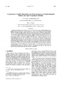


![[ ] [ ]H - Geophysical Fluid Dynamics Laboratory](https://m.moam.info/img/260x300/-h-geophysical-fluid-dynamics-laboratory_5c65c4f3097c47631a8b45b9.jpg)


