Cheng FH (F), Fan FT, Lai SH et al. Loop subdivision surface based progressive interpolation. JOURNAL OF COMPUTER SCIENCE AND TECHNOLOGY 24(1): 39–46 Jan. 2009
Loop Subdivision Surface Based Progressive Interpolation Fu-Hua (Frank) Cheng1 , Feng-Tao Fan1 , Shu-Hua Lai2 , Cong-Lin Huang1 , Jia-Xi Wang1 and Jun-Hai Yong3 (雍俊海) 1
Department of Computer Science, University of Kentucky, Lexington, KY 40506, U.S.A.
2
Department of Mathematics and Computer Science, Virginia State University, Petersburg, VA 23806, U.S.A.
3
School of Software, Tsinghua University, Beijing 100084, China
E-mail:
[email protected];
[email protected];
[email protected];
[email protected];
[email protected];
[email protected] Received June 4, 2008; revised December 11, 2008. Abstract A new method for constructing interpolating Loop subdivision surfaces is presented. The new method is an extension of the progressive interpolation technique for B-splines. Given a triangular mesh M , the idea is to iteratively upgrade the vertices of M to generate a new control mesh M such that limit surface of M would interpolate M . It can be shown that the iterative process is convergent for Loop subdivision surfaces. Hence, the method is well-defined. The new method has the advantages of both a local method and a global method, i.e., it can handle meshes of any size and any topology while generating smooth interpolating subdivision surfaces that faithfully resemble the shape of the given meshes. The meshes considered here can be open or closed. Keywords
1
geometric modeling, Loop subdivision surface, progressive interpolation
Introduction
Subdivision surfaces are becoming popular in many areas such as animation, geometric modeling and games because of their capability in representing any shape with only one surface. A subdivision surface is generated by repeatedly refining a control mesh to get a limit surface. Hence, a subdivision surface is determined by the way the control mesh is refined, i.e., the subdivision scheme. A subdivision scheme is called an interpolating scheme if the limit surface interpolates the given control mesh. Otherwise, it is called an approximating scheme. Popular subdivision schemes such as Catmull-Clark scheme[1] , Doo-Sabin scheme[2] , and Loop scheme[3] are approximating schemes while the Butterfly scheme[4] , the improved Butterfly scheme[5] and the Kobbelt scheme[6] are interpolating schemes. An interpolating subdivision scheme generates new vertices by performing local affine combinations on nearby vertices. This approach is simple and easy to implement. Because of its local property, it can handle meshes with a large number of vertices. However, since no vertex is ever moved once it is computed, any distortion in the early stage of the subdivision will persist.
This makes interpolating subdivision schemes very sensitive to irregularity in the given mesh. In addition, it is difficult for this approach to interpolate normals or derivatives. On the other hand, even though subdivision surfaces generated by approximating subdivision schemes do not interpolate their control meshes, it is possible to use this approach to generate a subdivision surface to interpolate the vertices of a given mesh. One method, called global optimization, does the work by building a global linear system with some fairness constraints to avoid undesired undulations[7,8] . The solution to the global linear system is a control mesh whose limit surface interpolates the vertices of the given mesh. Because of its global property, this method generates smooth interpolating subdivision surfaces that resemble the shape of the given meshes well. But, for the same reason, it is difficult for this method to handle meshes with a large number of vertices. To avoid the computational cost of solving a large system of linear equations, several other methods have been proposed. A two-phase subdivision method that works for meshes of any size was presented by Zheng and Cai for Catmull-Clark scheme[9] . A method
Regular Paper Research work presented here is supported by NSF of USA under Grant No. DMI-0422126. The last author is supported by the National Natural Science Foundation of China under Grant Nos. 60625202, 60533070.
40
J. Comput. Sci. & Technol., Jan. 2009, Vol.24, No.1
proposed by Lai and Cheng[10] for Catmull-Clark subdivision scheme avoids the need of solving a system of linear equations by utilizing the concept of similarity in the construction process. Litke, Levin and Schr¨oder avoid the need of solving a system of linear equation by quasi-interpolating the given mesh[11] . However, a method that has the advantages of both a local method and a global method is not available yet. In this paper a new method for constructing a smooth Loop subdivision surface that interpolates the vertices of a given triangular mesh is presented. The new method is an extension of the progressive interpolation technique for B-splines[12−16] . The idea is to iteratively upgrade the locations of the given mesh vertices until a control mesh whose limit surface interpolates the given mesh is obtained. It can be proved that the iterative interpolation process is convergent for Loop subdivision surfaces. Hence, the method is well-defined for Loop subdivision surfaces. The limit of the iterative interpolation process has the form of a global method. But the control points of the limit surface can be computed using a local approach. Therefore, the new technique enjoys the advantages of both a local method and a global method, i.e., it can handle meshes of any size and any topology while generating smooth interpolating subdivision surfaces that faithfully resemble the shape of the given meshes. The meshes considered here can be open or closed. The remaining part of the paper is arranged as follows. In Section 2, we present the concept of progressive interpolation for Loop subdivision surfaces on closed meshes. In Section 3, we prove the convergence of this iterative interpolation process. Extension of this technique to open meshes is considered in Section 4. Implementation issues and test results are presented in Section 5. Concluding remarks are given in Section 6.
between this vertex and its limit point V 0∞ on S 0 , D 0 = V 0 − V 0∞ , and add this distance to V 0 to get a new vertex called V 1 as follows: V 1 = V 0 + D0 . The set of all the new vertices is called M 1 . We then consider the Loop surface S 1 of M 1 and repeat the same process. In general, if V k is the new location of V 0 after k iterations of the above process and M k is the set of all the new V k ’s, then we consider the Loop surface S k of M k . We first compute the distance between V 0 and the limit point V k∞ of V k on S k D k = V 0 − V k∞ .
We then add this distance to V k to get V k+1 as follows: V k+1 = V k + D k .
Progressive Interpolation Using Loop Subdivision Surfaces for Closed Meshes
The concept of Loop subdivision surface based progressive interpolation for closed meshes can be described as follows. Given a closed 3D triangular mesh M = M 0 . To interpolate the vertices of M 0 with a Loop subdivision surface, one needs to find a closed control mesh M whose Loop surface passes through all the vertices of M 0 . Instead of finding the relationship between the vertices of M and the vertices of M 0 directly, we use an iterative process to do the job. First, we consider the Loop surface S 0 of M 0 . For each vertex V 0 of M 0 , we compute the distance
(2)
The set of new vertices is called M k+1 . This process generates a sequence of control meshes M k and a sequence of corresponding Loop surfaces S k . S k converges to an interpolating surface of M 0 if the distance between S k and M 0 converges to zero. Therefore the key task here is to prove that D k converges to zero when k tends to infinity. This will be done in the next section. Note that for each iteration in the above process, the main cost is the computation of the limit point V k∞ of V k on S k . For a Loop surface, the limit point of a control vertex V with valence n can be calculated as follows: V ∞ = βn V + (1 − βn )Q (3) where βn =
2
(1)
and
3 ³3 1 2π ´2 ´ 11 − 8 × + + cos 8 8 4 n ³3
(3)
n
1X Q= Q. n i=1 i
Qi are adjacent vertices of V . This computation involves nearby vertices only. Hence the progressive interpolation process is a local method and, consequently, can handle meshes of any size. Another point that should be pointed out is, even though this is an iterative process, one does not have to repeat each step strictly. By finding out when the distance between M 0 and S k would be smaller than the given tolerance, one can go directly from M 0 to M k , skipping the testing steps in between.
Fu-Hua (Frank) Cheng et al.: Loop Subdivision Surface Based Progressive Interpolation
3
Convergence of the Iterative Interpolation Process for Closed Meshes
The proof needs a fact about the eigenvalues of the product of positive definite matrices. This fact is presented in the following lemma. Lemma 1. Eigenvalues of the product of positive definite matrices are positive. Proof. The proof of Lemma 1 follows immediately from the fact that if P and Q are square matrices of the same dimension, then P Q and QP have the same eigenvalues (see, e.g., [17], p.14). To prove the convergence of the iterative interpolation process for Loop subdivision surfaces, note that at the (k + 1)-st step, the difference D k+1 can be written as: D k+1 = V 0 − V k+1 ∞ = V 0 − (βn V k+1 + (1 − βn )Qk+1 ) where Qk+1 is the average of the n adjacent vertices of V k+1 n 1 X k+1 Q . Qk+1 = n i=1 i By applying (2) to V
k+1
and each
Qk+1 , i
form: βn1
i
we get D k+1 = V 0 − (βn V k + (1 − βn )Qk ) n ³ 1 − βn X k ´ k D − βn D + n i=1 Qi n ³ 1 − βn X k ´ = D k − βn D k + D n i=1 Qi
where Qk is the average of the n adjacent vertices of V k . In matrix form, we have k D1 D k2 T , . . . , D k+1 , D k+1 [D k+1 m ] = (I − B) .. 2 1 . D km 0 D1 D 02 = (I − B)k+1 . ..
D 0m
where m is the number of vertices in the given matrix, I is an identity matrix and B is a matrix of the following
...
.. . 1 − βn i n i .. .
..
1 − βn1 n1
...
. ...
.
...
βni
···
βnm
The matrix B hasP the following properties: n 1) bij > 0, and j=1 bij = 1 (hence, kBk∞ = 1); 2) there are ni + 1 positive elements in the i-th row, and the positive elements in each row are equal except the element on the diagonal line; 3) if bij = 0 , then bji = 0. Properties 1) and 2) follow immediately from the formula of D k+1 in (3). Property 3) is true because if a vertex V i is an adjacent vertex to V j then V j is obviously an adjacent vertex to V i . Due to these properties, we can write the matrix B as B = DS where D is a diagonal matrix 1 − βn D=
Qik+1 = Qki + D kQk ,
41
n1 0 .. . 0
1
0
...
0
1 − βn2 n2
...
0
..
.
1 − βnm nm
and S is a symmetric matrix of the following form: n β 1 n1 ... 1 ... 1 − βn1 .. .. . . . S= n β i ni ... 1 ... 1 − βni .. nm βnm . 1 − βnm D is obviously positive definite. We will show that the matrix S is also positive definite, a key point in the convergence proof. ¤ Theorem 1. The matrix S is positive definite. Proof. To prove S is positive definite, we have to show the quadric form f (x1 , x2 , . . . , xm ) = X T SX is positive for any non-zero X = (x1 , x2 , . . . , xm )T . Note that if vertices V i and V j are the endpoints of an edge eij in the mesh, then sij = sji = 1 in the
42
J. Comput. Sci. & Technol., Jan. 2009, Vol.24, No.1
matrix S. Hence, it is easy to see that f (x1 , x2 , . . . , xn ) =
X
2xi xj +
eij
m X i=1
ni βni 2 x 1 − βni i
where eij in the first term ranges through all edges of the given mesh. On the other hand, if we use fijr to represent a face with vertices V i , V j and V r in the mesh, then since an edge in a closed triangular mesh is shared by exactly two faces, the following relationship holds: X
(xi + xj + xr )2 =
X eij
fijr
4xi xj +
m X
ni x2i
i=1
where fijr on the left hand side ranges through all faces of the given mesh. The last term in the above equation follows from the fact that a vertex with valence n is shared by n faces of the mesh. Hence, f (x1 , x2 , . . . , xn ) can be expressed as f (x1 , x2 , . . . , xn ) =
X1 fijr
+
2
(xi + xj + xr )2
m ³ X ni ´ 2 ni βni − xi . 1 − βni 2 i=1
nβn From (3), it is easy to see that 1−β > 53 n for n > 3. n Hence, f (x1 , x2 , . . . , xm ) is positive for any none zero X and, consequently, S is positive definite. ¤ Based on the above lemma and theorem, it is easy to conclude that the iterative interpolation process for Loop subdivision is convergent. Theorem 2. The iterative interpolation process for Loop subdivision surface is convergent. Proof. The iterative process is convergent if and only if absolute value of the eigenvalues of the matrix P = I − B are all less than 1, or all eigenvalues λi , 1 6 i 6 m, of B are 0 < λi 6 1. Since kBk∞ = 1, we have λi 6 1. On the other hand, since B is the product of two positive definite
matrices D and S, following Lemma 1, all its eigenvalues must be positive. Hence, the iterative process is convergent. ¤
4
Extension to Open Meshes
Loop subdivision surface based progressive interpolation technique can be used for open meshes as well. Actually the same advantages hold for open meshes too. Before we present Loop subdivision surface based progressive interpolation technique for open meshes, we need to review subdivision rules for the boundaries of an open mesh first. Two kinds of boundary rules have been presented for Loop subdivision in the literature[18−21] . In this paper, we follow the rules presented in [18, 19]. These rules, together with the Loop subdivision schemes, generate a smooth surface that is C 1 continuous at the boundaries[18,19] . For these rules to work, the vertices on the boundary are divided into two categories: regular vertices and extraordinary vertices. A boundary vertex is called a regular vertex if its valence is 4, as the one shown in Fig.1(a). Otherwise, a boundary vertex is called an extraordinary vertex. For each existing boundary vertex, a new vertex is computed as a linear combination of the existing vertex and its two neighbors with weights 3/4, 1/8 and 1/8, respectively. This vertex formula applies to both regular vertices and extraordinary vertices. For each boundary edge, a new edge vertex is generated in two ways. If the endpoints of the edge are both regular or both extraordinary, then the new vertex is just the average of the endpoints. If one of them is regular and the other one is extraordinary, then the new vertex is a linear combination of the regular vertex and the extraordinary vertex with weights 5/8 and 3/8, respectively, as in Fig.1(c).
Fig.1. (a) Regular vertex. (b)∼(d) Boundary subdivision rules. (e)∼(j) Limit point forumlas. The solid circular points are regular vertices and rectangle points are extraordinary vertices.
Fu-Hua (Frank) Cheng et al.: Loop Subdivision Surface Based Progressive Interpolation
Limit points are computed using two formulas, one for regular vertices and one for extraordinary vertices, as in Figs. 1(e) and 1(f). These formulas require both neighbors to be regular vertices. On boundaries of the initial mesh, one vertex could have either regular or extraordinary vertices. There are totally 6 different configurations. For each configuration, we can get a new limit point formula by combining the boundary subdivision rules with the standard limit points. These 6 limit point formulas are shown in Figs. 1(e)∼1(j). Note that boundary subdivision involves only the boundary vertices. Therefore interpolation can be performed for boundary vertices first. Once we have all the boundary vertices, interpolation of interior vertices is then performed without making any changes to the boundary vertices. The final mesh will interpolate both the boundary vertices and the interior vertices exactly. Interpolation of the boundary vertices is done using our progressive interpolation technique. The convergence of the interpolation is guaranteed. A mesh could have several disconnected closed boundaries, such as 6 in the pipe model in Fig.3(a). For each closed boundary, a linear system of equations can be built based on the limit point formulas for boundary vertices. VB∞ = EVB . Since every row is from one of the 6 limit point formulas, then E must be Pna strictly diagonally dominant matrix which means j=1,j6=i eij < eii . The eigenvalPn ues λi of E satisfy |λi | 6 1 for j=1 eij = 1. Thus the eigenvalues of E are in (0, 1]. The advantage of our technique is very desirable. No matter how many disconnected boundaries there are, interpolation is done for all boundaries at the same time just through the local geometric operations. It avoids explicitly solving several linear equations separately. Interpolation of interior vertices also uses the progressive interpolation technique. Its convergence is also provable. Let V = VB ∪ VI be the vertex set of the initial mesh M , where VB and VI are the set of boundary vertices and interior vertices, respectively. If we add one extra vertex q to M and connects every boundary vertices with q, we get an closed mesh M 0 with vertex set VC = V ∪ q. Applying the vertex limit point formula (3) to interior vertices, we get a linear equation: VI∞ = W V = WI VI + WB VB . WI is a submatrix of W consisting of |VI | columns of W corresponding to the interior vertices. WB is a similar submatrix corresponding to the boundary vertices. WI is similar to B for closed meshes. It can be
43
decomposed into one diagonal matrix DI and a symmetric matrix SI . For this new closed mesh M 0 , it is okay to apply the progressive interpolation technique developed in the previous sections. Therefore, the following equations hold. VC∞ = F VC That is,
VI∞ WI VB∞ = WB wq q∞
VI 0 0 VB . q αq
It is clear that W is just a submatrix of F . F is decomposed into DC and SC . SC depends only on the topology of the mesh. M is part of M 0 . Therefore, SI is just a minor of a positive definite matrix SC . Now it is clear that WI satisfies the convergent condition for progressive interpolation. The examples in Fig.3 show interpolation results of open meshes. 5
Results
The progressive interpolation process is implemented for Loop subdivision surfaces on a Windows platform using OpenGL as the supporting graphics system. Quite a few cases have been tested. Some of the closed cases (a hog, a rabbit, a tiger, a statue, a boy, a turtle and a bird) are presented in Fig.2. All the data sets are normalized, so that the bounding box of each data set is a unit cube. For each closed case, the given mesh and the constructed interpolating Loop surface are shown. The sizes of the data meshes, numbers of iterations performed, maximum and average errors of these cases are collected in Table 1. Table 1. Loop Surface Based Progressive Interpolation: Test Results Model
No. of Vertices
No. of Iterations
Max Error
Ave Error
Hog Rabbit Tiger Statue Boy Turtle Bird
606 453 956 711 17 342 445 1 129
10 13 9 11 6 10 9
0.000 870 799 0.000 932 857 0.000 720 453 0.000 890 806 0.000 913 795 0.000 955 765 0.000 766 811
0.000 175 255 0.000 111 197 0.000 141 480 0.000 109 163 0.000 095 615 0.000 172 600 0.000 088 345
Open mesh examples are shown in Fig.3. The performance is about the same as the closed mesh examples. For instance, for the face model (299 vertices) shown in Fig.3(c), it takes 10 iterations to reach an error of 0.000 998 516 for boundary vertex interpolation and also 10 iterations to reach an error of 0.000 896 328
44
J. Comput. Sci. & Technol., Jan. 2009, Vol.24, No.1
Fig.2. Examples of progressive interpolation using Loop subdivision surfaces (G-mesh ≡ given mesh; I-surface ≡ interpolating Loop surface). (a) (c) (e) (g) (i) (k) (m) G-mesh. (b) (d) (f) (h) (j) (l) (n) I-surface.
Fu-Hua (Frank) Cheng et al.: Loop Subdivision Surface Based Progressive Interpolation
45
References
Fig.3. Open mesh examples (I-surface ≡ interpolating Loop surface). Red solid dots are boundary vertices of the given mesh. (a) (c) Given mesh. (b) (d) I-surface. (e) Different view.
for interior vertex interpolation by the new pogressive interpolation technique. From these results, it is easy to see that the progressive interpolation process is very efficient and can handle large meshes with ease. This is so because of the expotential convergence rate of the iterative process. Another point that can be made here is, although no fairness control factor is added in the progressive iterative interpolation, the results show that it can produce visually pleasing surface easily. 6
Concluding Remarks
A progressive interpolation technique for Loop subdivision surfaces is presented and its convergence is proved. The limit of the iterative interpolation process has the form of a global method. Therefore, the new method enjoys the strength of a global method. On the other hand, since control points of the interpolating surface can be computed using a local approach, the new method also enjoys the strength of a local method. Consequently, we have a subdivision surface based interpolation technique that has the advantages of both a local method and a global method. The new technique works for both open and closed meshes. Our next job is to investigate progressive interpolation for CatmullClark and Doo-Sabin subdivision surfaces. Acknowledgement Triangular meshes used in this paper are downloaded from the Princeton Shape Benchmark[22] .
[1] Catmull E, Clark J. Recursively generated B-spline surfaces on arbitrary topological meshes. Computer-Aided Design, 1978, 10(6): 350–355. [2] Doo D, Sabin M. Behaviour of recursive division surfaces near extraordinary points. Computer-Aided Design, 1978, 10(6): 356–360. [3] Loop C. Smooth subdivision surfaces based on triangles [Master’ Thesis]. Dept. Math., Univ. Utah, 1987. [4] Dyn N, Levin D, Gregory J A. A butterfly subdivision scheme for surface interpolation with tension control. ACM Trans. Graphics, 1990, 9(2): 160–169. [5] Zorin D, Schr¨ oder P, Sweldens W. Interpolating subdivision for meshes with arbitrary topology. Computer Graphics, Ann. Conf. Series, 1996, 30: 189–192. [6] Kobbelt L. Interpolatory subdivision on open quadrilateral nets with arbitrary topology. Comput. Graph. Forum, 1996, 5(3): 409–420. [7] Halstead M, Kass M, DeRose T. Efficient, fair interpolation using Catmull-Clark surfaces. In Proc. SIGGRAPH 1993, Anaheim, USA, August 1–6, 1993, pp.47–61. [8] Nasri A H. Surface interpolation on irregular networks with normal conditions. Computer Aided Geometric Design, 1991, 8: 89–96. [9] Zheng J, Cai Y Y. Interpolation over arbitrary topology meshes using a two-phase subdivision scheme. IEEE Trans. Visualization and Computer Graphics, 2006, 12(3): 301–310. [10] Lai S, Cheng F. Similarity based interpolation using CatmullClark subdivision surfaces. The Visual Computer, 2006, 22(9): 865–873. [11] Litke N, Levin A, Schr¨ oder P. Fitting subdivision surfaces. In Proc. Visualization 2001, San Diego, USA, Oct. 21–26, 2001, pp.319–324. [12] de Boor C. How does Agee’s method work? In Proc. 1979 Army Numerical Analysis and Computers Conference, ARO Report 79-3, Army Research Office, pp.299–302. [13] Lin H, Bao H, Wang G. Totally positive bases and progressive iteration approximation. Computer & Mathematics with Applications, 2005, 50: 575–58. [14] Lin H, Wang G, Dong C. Constructing iterative non-uniform B-spline curve and surface to fit data points. Science in China (Series F), 2003, 47(3): 315–331. (in Chinese) [15] Qi D, Tian Z, Zhang Y, Zheng J B. The method of numeric polish in curve fitting. Acta Mathematica Sinica, 1975, 18(3): 173–184. (in Chinese) [16] Delgado J, Pe˜ na J M. Progressive iterative approximation and bases with the fastest convergence rates. Computer Aided Geometric Design, 2007, 24(1): 10–18. [17] Magnus I R, Neudecker H. Matrix Differential Calculus with Applications in Statistics and Econometrics. New York: John Wiley & Sons, 1988. [18] Hoppe H, DeRose T, Duchamp T, Halstead M, Jin H, McDonald J, Schweitzer J, Stuetzle W. Piecewise smooth surface reconstruction. In Proc. the 21st Annual Conference on Computer Graphics and Interactive Techniques (SIGGRAPH’94), Orlando, USA, July 24–29, 1994, pp.295–302. [19] Schweitzer J E. Analysis and application of subdivision surfaces [Ph.D. Dissertation]. University of Washington, Seattle, 1996. [20] Zorin D, Schr¨ oder P, DeRose T, Kobbelt L, Levin A, Sweldens W. Subdivision for modeling and animation. In SIGGRAPH 2000 Course Notes, ACM SIGGRAPH, Boston, USA, 2006, pp.30–50.
46
J. Comput. Sci. & Technol., Jan. 2009, Vol.24, No.1
[21] Biermann H, Levin A, Zorin D. Piecewise smooth subdivision surfaces with normal control. In Proc. SIGGRAPH 2000, New Orleans, USA, July 23–28, 2000, pp.113–120. [22] Shilane P, Min P, Kazhdan M, Funkhouser T. The Princeton shape benchmark. In Proc. Shape Modeling Int’l, June 7–9, 2004, pp.167–178.
Fu-Hua (Frank) Cheng is professor of computer science and director of the Graphics & Geometric Modeling Lab at the University of Kentucky. He holds a Ph.D. degree from the Ohio State University, 1982. His research interests include computer aided geometric modeling, computer graphics, parallel computing in geometric modeling and computer graphics, approximation theory, and collaborative CAD. He is on the editorial board of Computer Aided Design & Applications and Journal of Computer Aided Design & Computer Graphics.
Feng-Tao Fan is currently a Ph.D. candidate in the Department of Computer Science at the University of Kentucky. His research interests include computer graphics, geometric modeling, GPU techniques and computer vision.
Shu-Hua Lai is currently an assistant professor of computer science at the Virginia State University. He received his Ph.D. degree in computer science from the University of Kentucky in 2006. His research interests include computer graphics and computer aided geometric modeling.
Cong-Lin Huang is currently a Master candidate in the Department of Computer Science, the University of Kentucky. He received a B.S. degree in computer science from Sichuan University, China. His research interests include computer graphics, solid modeling and computer vision.
Jia-Xi Wang is currently working for Avnet, Inc. She received her B.E. degree of computer science from North China Electric Power University in 2005, and her M.S. degree of computer science from University of Kentucky in 2008. Her research interests include computer graphics and computer networks.
Jun-Hai Yong is currently a professor in School of Software at Tsinghua University, China. He received his B.S. and Ph.D. degrees in computer science from Tsinghua University, China, in 1996 and 2001, respectively. He held a visiting researcher position in the Department of Computer Science at Hong Kong University of Science & Technology in 2000. He was a post doctoral fellow in the Department of Computer Science at the University of Kentucky from 2000 to 2002. His research interests include computer-aided design, computer graphics, computer animation, and software engineering.
Fu-Hua (Frank) Cheng et al.: Loop Subdivision Surface Based Progressive Interpolation Fu-Hua (Frank) Cheng et al.: Loop Subdivision Surface Based Progressive Interpolation Fu-Hua (Frank) Cheng et al.: Loop Subdivision Surface Based Progressive Interpolation Fu-Hua (Frank) Cheng et al.: Loop Subdivision Surface Based Progressive Interpolation Fu-Hua (Frank) Cheng et al.: Loop Subdivision Surface Based Progressive Interpolation Fu-Hua (Frank) Cheng et al.: Loop Subdivision Surface Based Progressive Interpolation