Lop to model concurrent MPI communications in multicore clusters

Future Generation Computer Systems 61 (2016) 66–82

Contents lists available at ScienceDirect

Future Generation Computer Systems journal homepage: www.elsevier.com/locate/fgcs

Extending τ -Lop to model concurrent MPI communications in multicore clusters Juan-Antonio Rico-Gallego a,∗ , Juan-Carlos Díaz-Martín a , Alexey L. Lastovetsky b a

University of Extremadura, Avd. Universidad s/n, 10003, Cáceres, Spain

b

University College Dublin, Belfield, Dublin 4, Ireland

highlights • • • • •

We present an extension of the τ -Lop performance model for multicore clusters. The τ -Lop goal is to help in the design and optimization of parallel algorithms. It is applied to collective algorithms in mainstream MPI implementations. The τ -Lop model is compared to other well known and established models. A methodology is described for the measure of the parameters of the model.

article

info

Article history: Received 30 September 2015 Received in revised form 27 January 2016 Accepted 27 February 2016 Available online 11 March 2016 MSC: 00-01 99-00 Keywords: Parallel performance models Parallel algorithms Message passing interface Performance analysis Multicore clusters

abstract Achieving optimal performance of MPI applications on current multi-core architectures, composed of multiple shared communication channels and deep memory hierarchies, is not trivial. Formal analysis using parallel performance models allows one to depict the underlying behavior of the algorithms and their communication complexities, with the aims of estimating their cost and improving their performance. LogGP model was initially conceived to predict the cost of algorithms in mono-processor clusters based on point-to-point transmissions with network latency and bandwidth based parameters. It remains as the representative model, with multiple extensions for handling high performance networks, covering particular contention cases, channels hierarchies or protocol costs. These very specific branches lead LogGP to partially lose its initial abstract modeling purpose. More recent logn P represents a point-to-point transmission as a sequence of implicit transfers or data movements. Nevertheless, similar to LogGP, it models an algorithm in a parallel architecture as a sequence of message transmissions, an approach inefficient to model algorithms more advanced than simple treebased one, as we will show in this work. In this paper, τ –Lop model is extended to multi-core clusters and compared to previous models. It demonstrates the ability to predict the cost of advanced algorithms and mechanisms used by mainstream MPI implementations, such as MPICH or Open MPI, with high accuracy. τ –Lop is based on the concept of concurrent transfers, and applies it to meaningfully represent the behavior of parallel algorithms in complex platforms with hierarchical shared communication channels, taking into account the effects of contention and deployment of processes on the processors. In addition, an exhaustive and reproducible methodology for measuring the parameters of the model is described. © 2016 Elsevier B.V. All rights reserved.

1. Introduction Modern high performance computing systems are composed of nodes with a significant number of cores per node and deep

∗

Corresponding author. E-mail addresses: [email protected] (J.-A. Rico-Gallego), [email protected] (J.-C. Díaz-Martín), [email protected] (A.L. Lastovetsky). http://dx.doi.org/10.1016/j.future.2016.02.021 0167-739X/© 2016 Elsevier B.V. All rights reserved.

memory hierarchies, connected by high performance networks. Scientific applications face the challenge of obtaining as much performance as possible from such complex platforms. MPI [1] is the de facto standard that defines the communications interface used by this type of applications. The MPI execution model is based on processes communicating by message passing, including point-to-point and collective operations, which involve a group of processes. Frequently used [2], collective operations are a key issue in achieving performance and scalability in parallel applications.

J.-A. Rico-Gallego et al. / Future Generation Computer Systems 61 (2016) 66–82

A collective operation can be implemented by algorithms from a preset menu, with one of them chosen at runtime based on the value of parameters such as message length or group size. In general, an algorithm is executed as a sequence of steps, and defines a point-to-point communication graph between the processes of the group. Algorithms are designed with the goals of minimizing the number of such steps, optimizing the use of the underlying communication channels available in the system, or fitting a particular network technology or topology. Besides, achieving these goals in modern complex multi-core clusters requires to consider the hierarchy of communication channels (imposed by the difference in channels performance), the implications of process distribution over the cores of the platform (virtual topology), and the contention effects due to the use of shared communication resources. Parallel performance models provide a theoretical framework for analytic representation of the communications and their associated costs, based on system parameters. Important features including advanced transmission mechanisms (such as RDMA and OS bypass), middleware related costs, or network technology, should be captured by an accurate and scalable cost estimation model. The type of parameters divides the known models in two broad groups: hardware and software. Hardware models, such as Hockney [3] or LogP [4], represent communication costs with hardware related parameters, such as network latency or bandwidth. They were initially created for homogeneous monoprocessor clusters, and the increasing complexity of modern platforms limits their accuracy. In addition, they show weakness in representing different mechanisms provided by the software such as communication protocols, or in estimating the impact of the communication middleware on the communication cost. These issues are partially addressed by adding new parameters for such protocols in LogGPS [5] or hierarchical communications in LogGPH [6]. By contrast, software models, such as logn P [7,8], abstract the hardware complexities by the adoption of parameters related to the communication middleware, with the drawback of a possible loss of network technology details. τ -Lop [9] is a software parametrized parallel model aimed to represent parallel algorithms and accurately and scalably predict their cost. It provides a simple and powerful abstraction by considering a message transmission as a sequence of transfers. The transfers reflect data movements between hardware or software agents, and are modeled based on the underlying architecture characteristics. The decomposition of a message transmission into a sequence of transfers allows for an incremental analysis of the algorithm, from a high level representation to low platform-specific details. For instance, a point-to-point message transmission could be used as the building block to model a collective operation, but deeper insight can be obtained by further considering the transmission as a sequence of data transfers. The decomposition of a point-to-point message transmission into transfers is not a new concept [10]. τ -Lop goes beyond in natively representing the concurrency in the access to the channel when it is shared by parallel transfers. This contention effect has a significant impact on the algorithm performance, so that its consideration in the model results in a substantial improvement in the accuracy of the predicted cost. The contribution of this paper is the extension of τ -Lop, which was initially developed to model the behavior of collective algorithms in shared-memory compute nodes, to modern multicore clusters. Furthermore, the extended τ -Lop model addresses the influence on the cost of the deployment of processes over the system processors. In a multi-core cluster with hierarchical organization of communication channels, the mapping of processes can improve

67

or aggravate the contention effect. τ -Lop takes into account the way the virtual topology defined by the algorithm is mapped onto the physical topology of the machine. This ability provides a more realistic representation of the algorithm, leading to a better cost prediction. The rest of the paper is structured as follows. Section 2 revisits the state-of-the-art models, with emphasis on LogGPH and mlogn P, later used in cost evaluations. Section 3 describes the τ -Lop model and its extensions to cover multi-core clusters. Section 4 discusses its application to key algorithms of MPI collectives in multi-core clusters and demonstrates its potential as an analytical inference model for prediction of the communication cost. Section 5 addresses the communication modeling of a whole application, a parallel matrix multiplication kernel on a multi-core cluster. Section 6 gives details of the experimental approach used to estimate the parameters of the model, and Section 7 concludes the paper. An Appendix is included to describe the approach to report the error measurements. 2. Related work Most of the current parallel performance models derive from Hockney [3] and Culler et al. LogP [4]. Both are linear models, in the sense that they represent the point-to-point communication cost by a linear function of the size of the message. Hockney represents the cost as T = α + m β , where m is the size of the message, α is the network latency, and β is the inverse of the network bandwidth. The execution time of a parallel algorithm in the cluster is formulated in terms of these parameters. Together with benchmarks measurements, this simple model has been used for comparison of different MPI collective algorithms in a given system, for ranges of message sizes and numbers of involved processes [11,12]. The more advanced LogP cost model splits the network latency in the network delay (L) and the network overhead (o). The overhead is the time invested by the processor in sending and receiving a message. This separation of processor and network contribution allows one to model the computation and communication overlap. LogP also includes the minimum time interval between message transmissions as g. Alexandrov et al. LogGP model [13] extends LogP with an additional parameter, G, that captures the network bandwidth for long messages. It represents the cost of a single point-to-point message transmission as: TLogGP = L + 2 o + (m − 1) G. Several models drawn from LogGP contribute with a variety of add-ons to represent different aspects of the communication in complex HPC platforms. LogGPS [5] covers aspects of synchronization, providing the rendezvous cost as a new parameter, LogGPH [6] supports representation for hierarchical architectures through a different set of parameter values for each communication channel, LoGPC [14] adds contention time in mesh networks, and LogGPO [15] accurately captures the overlap of communication and computation in non-blocking transmissions. Linear models have proven their ability to model point-to-point message transmissions, as shown by Al-Tawil et al. in [16], and upon them, the message passing algorithms underlying the collective primitives of the MPI standard on mono-processor clusters [17,18]. Analytical modeling of a broad range of these algorithms using the Hockney model can be found in [12,19] and [11]. An optimal broadcast algorithm is developed in [20], and in [21] for heterogeneous networks, the gather collective is addressed in [22] and [23], algorithms for reduction operations are developed in [24], and for the Alltoall collective in [25].

68

J.-A. Rico-Gallego et al. / Future Generation Computer Systems 61 (2016) 66–82

In the work by Pješivac-Grbović et al. [17], parallel algorithms are also modeled using PLogP [26]. The Parametrized LogP model slightly changes the meaning of some parameters of LogP and makes them (except latency) dependent on message size. This model is applied to a wide range of collective algorithms in [27]. Lastovetsky et al. LMO [28,29] is a parallel performance model aimed to estimate the cost of algorithms in heterogeneous, in addition to homogeneous, systems. Similar to LogGP, it carefully separates the cost related to the processors and the network in order to gain more accurate communication cost predictions, and it is evaluated for a limited set of collectives: broadcast, scatter and gather. More specific costs models fitting different network technologies also exist. Hoefler et al. LogfP [30] models short messages in Infiniband networks. The authors use the model to study the effects of multi-stage switches on that kind of networks in [31]. Paper [32] analytically estimates the communication delays in Myrinet networks, and the work in [33] addresses hierarchical Ethernet networks. Nevertheless, the increasing complexity of multi-core cluster architectures and the implementation of different intra-node communication techniques by current MPI libraries lead to the necessity of new approaches. The model logn P [7,8] by Cameron et al. has nothing to do with LogP, although they are similar in name. logn P was also conceived, just as LogP, to model point-to-point communication, but with a new key feature, each individual data transfer that occurs in a message transmission. mlogn P [34] extends logn P by distinguishing the variety of communication channels in a system, such as intra-socket, inter-socket and network. mlogn P represents the cost of a point-to-point transmission of a message of a given size through the communication channel1 c as: n c −1 c Tmlog nP

=



ocj

(1)

j =0

n = {n0 , n1 , . . . , nm−1 } is a vector with one component per communication channel (nc ) indicating the number of transfers a message experiences to reach the destination buffer. m is the number of communication channels in the system. The overhead, oc , is the time the processor invests in each transfer composing the message transmission. In multi-core clusters with m = 2, such as those of Section 6.1, communicating two processes usually implies two transfers in the shared memory communication channel, through an intermediate buffer. However, when the processes run in different nodes, three transfers will take place, namely one transfer from the source buffer to the NIC, another transfer through the network to the destination NIC, and finally a third transfer to the receive buffer. Hence, the number of transfers through each of the m = 2 channels is represented by the vector n = {2, 3}, i.e., two transfers through channel number 0 (shared memory) and three transfers through channel number 1 (network). Definition (1) is applied using tailored 2log{2,3} P model to represent the cost of a transmission in shared memory as: n 0 −1 0 Tmlog nP

=



o0j = o00 + o01 = omw .

j =0

Note that in shared memory the two transfers have the same cost, and their addition is represented as omw (middleware overhead). In the network channel, first and last transfers have the same cost,

1 Term channel is used in this paper instead of the original lev el used in mlog P n model.

whose contribution is represented as o′mw . The intermediate transfer, between NICs, progresses through the network and its cost is o′net : n 1 −1 1 Tmlog nP

=



o1j = o10 + o11 + o12 = o′mw + o′net .

j =0

In the authors’ view, the transfer is the building block that conveniently suits the purpose of modeling the behavior of MPI algorithms in shared memory, and also in networks. Notwithstanding, logn P and mlogn P have not demonstrated enough their capabilities to model and predict the cost of collective MPI algorithms, beyond some basic broadcast algorithms. Regarding contention modeling, a sound work studying this issue in high performance networks is carried out in [35] for Infiniband and in [36,37] for Ethernet and Myrinet networks. The authors generate specific models for each type of network based on the study of network flow control mechanisms and experimentally deduce penalty coefficients, derived from resource sharing experiments, and categorize different types of conflicts. Paper [38] shows that contention derived from bidirectional TCP communication in a full-duplex Ethernet network diminishes the maximum reachable network bandwidth. LoGPC [14] introduces a large set of parameters to evaluate contention in mesh networks with wormhole routing. Work [39] introduces the contention factor, represented as a parameter exclusively affecting the network performance, which is incremented linearly from the content-free communication cost. The former work evaluates the total exchange collective under this assumption. In general, contention-aware studies provide hardware models very close to the specific network technology. They usually deal with a limited number of nodes and, even more important, with a small number of cores per node. These works do not address the shared memory effects in the overall communication cost and, hence, omit the impact of the virtual topology of processes on the cost of the collective algorithms. Besides, again only a limited set of simple collectives have been evaluated against the generated models. Work [9] addresses the contention representation, as well as the cost prediction of a range of collective algorithms in large shared memory systems, either built upon point-to-point communication primitives or not, using the τ -Lop model. The model is applied to two cases of study in [40], including the analysis of the cost introduced by the network contention in the Allgather collective operation. This paper extends the τ -Lop model to represent and empirically study the contention in clusters. They combine communication channels which are different in bandwidth and behavior. We show that the representation of cost is both simple and generic, and flexible enough to cover network specific details as needed. 3. The τ -Lop model

τ -Lop is a software parametrized model with the goals of representing the behavior of parallel algorithms, specially those used in MPI collective operations, and accurately and scalably predicting their cost. τ -Lop models the communications of an algorithm as a sequence of transfers (data copies), progressing concurrently through the communication channels of the system. 3.1. Modeling a transmission The cost of a point-to-point transmission of a message of size m through the communication channel c, is represented as: c Tp2p (m) = oc (m) +

s −1  j=0

Lcj (m, τj ).

J.-A. Rico-Gallego et al. / Future Generation Computer Systems 61 (2016) 66–82

69

0 Fig. 1. A shared memory transmission Tp2p (m) of a message divided up in k = 3

segments of size S. It needs a total of 6 transfers (L0 ) and 4 steps.

The transfer time of a message of size m, L(m, τ ), is the cost of τ transfers contending for the communication channel. A transmission is composed of s steps, and its cost is calculated as the addition of their transfer times and the overhead. Overhead o includes the cost of the protocol agreement for the communication and the software stack. In the shared memory channel (c = 0), a point-to-point transmission between two processes goes through buffers in a common memory zone, and hence, it needs two transfers (s = 2), from the sender buffer to the intermediate buffer, and then to the receiver buffer, with the cost: 0 Tp2p (m) = o0 (m) + 2 L0 (m, 1).

(2)

The number of transfers s in a transmission, notwithstanding, depends on the platform. In shared memory, the operating system allows the direct movement of data between two processes in just one transfer, for instance, using KNEM [41] or LiMIC [42] kernel modules in MPI, and high performance networks reduce the number of transfers through the use of RDMA (Remote Direct Memory Access) mechanisms [43]. In τ -Lop, two transfers are concurrent when they share the communication channel. Concurrent transfers generate a contention in the channel that has an impact on the overall communication cost. For instance, the transmission of a large message in shared memory is done in most libraries by splitting the message in k segments of a constant size S, with k = m/S. Thus, the writing of segments from the sender buffer to the intermediate shared area progresses concurrently with the writing to the receiver buffer, as shown in Fig. 1. The cost of the whole message transmission between S and R is modeled by τ -Lop as2 : 0 Tp2p (m) = o0 (m) + 2 L0 (S , 1) + (k − 1) L0 (S , 2).

(3)

L0 (S , 2) is the cost of the intermediate segment transfers, in which the sender and receiver processes access simultaneously the communication channel, and hence, share the channel bandwidth. Note that, when m ≤ S, the cost becomes represented by expression (2). The definition of the transfer time enforces the restriction that the cost of A concurrent transfers will be some value between the cost of a single transfer and that of A consecutive ones, Lc (m, 1) ≤ Lc (m, A) ≤ A × Lc (m, 1), an expression that is generalized for convenience as follows: Lc (m, τ ) ≤ Lc (m, A × τ ) ≤ A × Lc (m, τ ).

(4)

2 Note that the number of steps needed to transmit a segmented message is s = k + n − 1, with n the number of copies needed by a byte to reach the destination. The total number of transfers is k × n.

Fig. 2. Short messages completion time of concurrent (τ ) transmissions in network (TCP/Ethernet) communication channel, as a function of the message size (shown at the right).

As well, as assumed by most models, the transfer time cost grows linearly with the increase of the message size, named the linearity principle, and hence: Lc (A × m, τ ) = A × Lc (m, τ ).

(5)

Regarding the network channel, τ -Lop follows the same scheme by Cameron et al. in [8] for an Ethernet network, which considers a message transmission between two processes as composed of three transfers: first, from the sender buffer to the internal buffer of the NIC in the sender node, second, to the NIC in the receiver node, and last, to the receiver buffer. The first and last are shared memory transfers (with cost L0 ), whereas the second transfer progresses through the network (with cost L1 ). The cost of an inter-node message transmission is hence represented as: 1 Tp2p (m) = o1 (m) + 2 L0 (m, 1) + L1 (m, 1).

(6)

Similar to the shared memory case, the number of transfers of a network transmission depends on the specific platform, a fact that allows some variations to (6). For instance, some networks as Infiniband allows the direct transfer of data from the sender buffer to the receiver buffer using a Remote Direct Memory Access (RDMA) mechanism. The cost of this direct point-to-point transmission is represented as: 1 Tp2p (m) = o1 (m) + L1 (m, 1).

(7)

3.2. Modeling concurrent transmissions Real MPI collective operations include message transmissions that share the communication channel bandwidth. The contention increases the cost of each individual transmission. Figs. 2 and 3 show the growth of the cost of a single transmission with the increase of the number of concurrent transmissions τ in the network channel. Section 6.1 shows that the impact of the concurrency on the cost is significant when the size of message is greater than 2KB in the test system. In shared memory, the effect of concurrency is similar, as deeply studied in [9]. τ -Lop represents the concurrency of point-to-point transmissions by using the ∥ operator. The cost of A parallel transfers of size m is represented as A ∥ Lc (m, 1) = Lc (m, A), and more generally, A ∥ Lc (m, τ ) = Lc (m, A×τ ). Definition of ∥ is extended to cover the cost of concurrent message transmissions. Expression A ∥ T c (m) represents the cost of A concurrent transmissions T of a message of size m contending for the communication channel c. Fig. 4 shows two point-to-point transmissions concurrently progressing through the shared memory channel. Each transmission, with the cost defined by (2), is composed of two transfers

70

J.-A. Rico-Gallego et al. / Future Generation Computer Systems 61 (2016) 66–82

Fig. 5. τ -Lop cost analysis of two concurrent transmissions from node M#0 to node M#1. Fig. 3. Large messages completion time of concurrent (τ ) transmissions in network (TCP/Ethernet) communication channel, as a function of the message size (shown at the right).

Fig. 4. Cost of the concurrency of two transmissions in shared memory through a intermediate buffer expressed in terms of τ -Lop.

actually contending for the communication channel, leading to an increase in the cost, modeled in τ -Lop as: 0 2 ∥ Tp2p (m) = 2 ∥ o0 (m) + 2 L0 (m, 1) = o0 (m) + 2 L0 (m, 2).





Note that the overhead cost is attributable to the processor, a nonshared resource, and hence not affected by ∥. Fig. 5 shows an example of two concurrent point-to-point transmissions through the network communication channel. Analysis of the contention shows that transfers in the node (M#i) between the source buffer and the NIC progress concurrently, hence with cost L0 (m, 2). Data sent through the network has the same destination node (M#j), therefore, contention is generated in the destination NIC, with cost L1 (m, 2). Finally, the data is transferred from the NIC to the destination buffers (L0 (m, 2)). The total cost is: 1 2 ∥ Tp2p (m) = 2 ∥ o1 (m) + 2 L0 (m, 1) + L1 (m, 1)





= o1 (m) + 2 L0 (m, 2) + L1 (m, 2). For the sake of simplicity, the analysis in this paper makes two assumptions regarding network transfers. First, it does not consider the overlap of the transfer from a buffer to the local NIC with the transfer from the local NIC to the remote NIC, assuming, in common with most of the models, the error in the prediction. Such concurrency has a random behavior difficult to measure and highly dependent on the network technology. Second, the only network transfers considered as concurrent are those reaching the same destination node at the same time, hence contending in the destination NIC. The impact of concurrency on the cost of the transfers from NIC to NIC is hardware dependent, and so is considered in τ -Lop. In any case, the flexibility of the model allows itself to adapt to any other system characteristics found in other high performance platforms. For an exhaustive taxonomy of contention effects in high performance networks, see work by Jerome et al. in [37].

4. Collective algorithms This section evaluates the τ -Lop capability to model three well-known algorithms widely used in MPI collective operations: Binomial Tree, Ring and Recursive Doubling. Each algorithm is executed in a sequence of stages, where the number of involved processes and the message size may change along the stages. The accuracy, scalability and expressiveness of τ -Lop in the algorithm modeling are compared to that of LogGPH and mlogn P. Each algorithm involves P processes, ranked in the range 0 . . . P − 1, deployed over the multi-core cluster. The experiments are conducted in Metropolis, a multi-core cluster using Gigabit Ethernet (see Section 6.1). Two communication channels are considered, shared memory and network. Considering that the mapping of processes to the system processors determines the used communication channels, the algorithm performance highly depends on the chosen mapping. This paper considers by default sequential mapping, that is, process with rank i runs in the processor i % Q of the node i ÷ Q , with Q the number of cores per node or, in simple words, ranks fill each node before going to the next one. Nevertheless, extension to other mappings is straightforward. M represents the number of nodes in the cluster. 4.1. Binomial Tree In the Binomial Tree algorithm a process named root broadcasts a message to the rest of processes. In the first stage, the root sends the message of size m to the process with rank root + P /2. The algorithm recursively continues with both processes acting as roots of sub-trees with P /2 processes. The number of stages is the height of the tree (⌈log2 P ⌉). The number of sending processes doubles in each stage, whereas the message size remains constant. LogGPH and mlogn P estimate the algorithm cost as the height of the tree multiplied by the cost of a point-to-point transmission. Fig. 6 shows the generated message transmissions in a theoretical multi-core cluster composed of P = 16 processes arranged in sequential mapping on M = 4 nodes. As can be distinguished, the number of stages transmitting data through the network channel is log2 M, while the number of stages with data transmissions through shared memory is log2 Q , with Q = P /M being the number of processes in each node. Adding both costs, the LogGPH estimation is: 1 0 TBin,LogGPH = log2 M · TLogGPH + log2 Q · TLogGPH .

(8)

0 1 Note that TLogGPH ̸= TLogGPH , because the values of the L, o and G parameters are different in each communication channel (as proposed in the LogGPH model), making the mapping of processes a key factor in the performance of the algorithm in a multi-core cluster.

J.-A. Rico-Gallego et al. / Future Generation Computer Systems 61 (2016) 66–82

Fig. 6. A Binomial Tree with P = 16 processes (root = 0) deployed in M = 4 nodes with sequential mapping. Transmissions through different communication channels are shown, shared memory (dotted line) and TCP (bold line). M#j indicates the machine where the process runs.

71

Fig. 7. Estimation of the cost of a Binomial Tree compared to its real cost in MPICH in terms of bandwidth. Number of processes is P = 32, deployed sequentially on M = 4 nodes in Metropolis.

mlogn P natively models different communication channels, and estimates the cost as: TBin,mlogn P = log2 M · o′mw + o′net + log2 Q · omw .





(9)

The contention highly depends on the deployment of the processes in the system. Take as an example the last stage (s#3) of Fig. 6, where two transmissions arrive concurrently to each node. Unlike LogGPH and mlogn P, τ -Lop models the impact of mapping and the resulting contention on the cost of an algorithm. The cost of the binomial tree will be represented as:

ΘBin (m) =

⌈log 2 (P )⌉−1



map

Ci

 c ∥ Tp2p (m) .

(10)

i =0 c Tp2p (m) is the cost of a point-to-point transmission through the communication channel c, and is defined in (3) for shared memory map and in (6) for the network. Ci is the maximum number of concurrent transmissions through the communication channel used in the stage i, determined by the process mapping (map). In the first stage, there is a point-to-point transmission through the 1 network, with cost 1 ∥ Tp2p (m). In the second stage (s#1) there are two transmissions progressing through the network channel. As the sequential mapping causes that their destination nodes are 1 different, no contention takes place, and cost is 1 ∥ Tp2p (m). The third stage has four transmissions in shared memory, scattered 0 in different nodes, with cost 1 ∥ Tp2p (m). In the last stage, there will be two concurrent shared memory transmissions in each node, SEQ 0 therefore, C3 = 2 and the stage cost is 2 ∥ Tp2p (m). The total cost will be: 1 0 0 ΘBin (m) = 2 Tp2p (m) + Tp2p (m) + 2 ∥ Tp2p (m).

(11)

Fig. 7 shows the execution bandwidth of the binomial tree used by the MPI_Bcast collective operation of MPICH, with increasing message sizes and P = 32 processes distributed sequentially in the M = 4 nodes of the Metropolis platform. MPICH measured bandwidth is compared to the estimations derived from (8), (9) and (11). The bandwidth is used, instead of the completion time, for reasons of clarity in the graph, and calculated as m/t, with m being the size of the message and t being the cost time returned by the models. Parameters of the models are measured as explained in Section 6. In our view, LogGPH is not suitable to model shared memory communications. The reason is that parameters of the model are bound to network hardware. Nonetheless, it is one of the most extended models, although it does not show a good accuracy in this configuration. The difference between mlogn P and τ -Lop is small, because the sequential mapping causes a minimal contention

Fig. 8. Proportional error in the cost estimation over a range of medium and large message lengths. Process number is P = 32, deployed sequentially on M = 4 nodes in Metropolis.

in this algorithm. In the range of large messages, however, τ Lop shows a slightly better fit, derived from the shared memory contention. Fig. 8 reinterprets the Fig. 7 to show the proportional error, µ (see Appendix), in the estimation of the cost by models with respect to the real MPICH measured value. mlogn P and τ -Lop have a similar error, near to the optimum value µ = 1. Fig. 9 represents the mean proportional error in the range of message sizes of Fig. 8 when the number of processes grows. The cost estimation of the binomial is scalable, that is, there has been no increase in error with the increase of the number of processes, because of the minimal contention of the algorithm in the Metropolis small test platform. 4.2. Ring This section evaluates the Ring algorithm. It is often used in the MPI_Allgather collective operation, as well as in MPI_Bcast and MPI_Alltoall. It is composed of an initial local copy and P − 1 stages. Each process makes the initial copy of m bytes from its input to its output buffer, with offset p × m. In each stage, the process with rank p sends to the process with rank (p + 1) mod P the m bytes received in the previous stage. The number of processes and the message size remain constant along the stages, all of them equal. Fig. 10 represents the intra- and inter-node transmissions generated by the algorithm under sequential mapping. LogGPH and mlogn P estimate the cost of a stage as the addition of the most

72

J.-A. Rico-Gallego et al. / Future Generation Computer Systems 61 (2016) 66–82

Fig. 11. A short message transmission in a Ring algorithm. Processes are mapped sequentially. Transfers in node M#0 are deployed.

Fig. 9. Mean proportional error in the cost estimation of a Binomial Tree with increasing number of processes per node (Q = P /M) in the Metropolis platform.

Fig. 10. Representation of the transmissions of the Ring algorithm in a hypothetical machine with M = 4 nodes and P = 16 processes arranged in sequential mapping.

expensive send and receive for a process. Excluding the negligible cost of the initial shared memory copy, the algorithm cost will be: TRing ,LogGPH (m) = (P − 1) ×



L0 + 2 o0 + (m − 1) G0

+ L1 + 2 o1 + (m − 1) G   TRing ,mlogn P (m) = (P − 1) × omw + o′mw + o′net . 

 1

 (12) (13)

As the sequential mapping divides evenly the network transmissions among the nodes (see Fig. 10), the algorithm communication pattern avoids contention in the network channel. Nevertheless, contention in shared memory affects the final cost of the algorithm, and the impact grows with the increase of the number of processes per node (Q ). In each stage, a rank sends a message to the next rank and receives a message from the previous rank by invoking the MPI_Sendrecv operation. The Send–receive operation cost is represented as Tsr (m), and executed by P processes through a shared communication channel c. It has the cost of P c concurrent point-to-point transmissions Tsrc (m) = P ∥ Tp2p (m). Actually, in the multi-core platform, the destination and the source rank of both transmissions can be in the same or different node, therefore, they could progress through shared memory or network. τ -Lop models the Ring algorithm as follows:

  ΘRing (m) = (P − 1) × C map ∥ Tsr (m) , map

where C is the maximum number of concurrent transmissions in each stage. In the sequential mapping of Fig. 10, it will have the same value along all stages, C SEQ = Q . How will Tsr (m) be affected by C SEQ ? Next, two scenarios are discussed that lead to different cost representations depending on the message size. For short messages, as represented in Fig. 11, two types of transmissions mix in each stage of the Ring algorithm. We discuss the scenario at transfer level. The first transfer of all processes,

Fig. 12. Estimation of the cost of Ring Allgather with three models, compared to the real MPICH measurements. Number of processes is P = 32, deployed on M = 4 nodes in Metropolis.

either to the NIC or to the intermediate buffer, progresses through shared memory, hence, the transfer cost will be L0 (m, Q ). Next, a network transfer of one process per node starts while the rest of processes (Q − 1) complete the communication through shared memory. These inter- and intra-node transfers progress through different communication channels, and hence, they do not contend, leading to a cost represented as max{L0 (m, Q − 1), L1 (m, 1)}. Note that L1 (m, 1) ≫ L0 (m, Q − 1) in the platform evaluated, with Q ≤ 8 (see Section 6.1). This analysis should change according to the network technology and the number of processes per node, given sequential mapping. Finally, the last transfer is done by only one receiver process per node from the network (represented as rank P0 in Fig. 11). Thus, the total cost will be:

  ΘRing (m) = (P − 1) × L0 (m, Q ) + L1 (m, 1) + L0 (m, 1) .

(14)

For long messages, MPI_Sendrecv is modeled as a sequence of two point-to-point transmissions. First, the shared memory transmission segments the message, hence requires the involvement of both the sender and the receiver processes as discussed in Sec0 tion 3.1. The cost will be Q ∥ Tp2p (m). Second, the network transmission is performed by a single process per node, hence without 1 (m). The total cost will be as folcontention, with the cost of Tp2p lows:

  0 1 ΘRing (m) = (P − 1) × Q ∥ Tp2p (m) + Tp2p (m) .

(15)

Fig. 12 shows the bandwidth cost of the Ring algorithm implemented in the MPI_Allgather collective operation of MPICH, for different message sizes and P = 32 processes deployed in M = 4 nodes. The measured value is compared to (12), (13) and (14), (15). Although the impact of contention on the cost is small in the Ring algorithm with sequential mapping, because it occurs in shared memory, τ -Lop better fits the real measurements than mlogn P over

J.-A. Rico-Gallego et al. / Future Generation Computer Systems 61 (2016) 66–82

73

Fig. 13. Proportional error of the Ring estimation cost for a range of medium and large message lengths. P = 32 processes deployed in M = 4 nodes in Metropolis.

Fig. 15. Stages of the Recursive Doubling Algorithm with P = 16 processes deployed sequentially in M = 4 nodes. A double-headed arrow represents a message interchange of the specified size, which is modeled in τ -Lop as Texch . The number of concurrent interchanges between nodes in the inter-node s#2 and s#3 stages is shown in parenthesis.

The LogGPH cost of RDA in a given channel is the addition of the cost of each stage [17], as: TRDA,LogGPH =

⌈log 2 (P )⌉−1

TLogGPH 2i m





i=0

= log2 P · (L + 2 o − G) + (P − 1) m G. Fig. 14. Mean proportional error of the Ring for increasing number of processes deployed on M = 4 nodes in Metropolis.

the entire message range. The difference in predictions by the models slightly increases in comparison with that for the broadcast in Fig. 7, due to increase in shared memory contention. Fig. 13 shows the proportional error made by the models as compared with the real MPICH measurements. Fig. 14 shows the proportional error for the range of message sizes in previous figure, for increasing number of processes. Modeling the cost of the Ring algorithm, with transmissions that progress concurrently through two channels, is a complex task. All models underestimate the shared memory contention influence due to the fact that, compared to network transmissions, the shared memory cost is low. Nevertheless, the cost should become significant when Q increases. Although the τ -Lop proportional error is not too high, further in-depth analysis at the transfer level for each particular platform should decrease it. 4.3. Recursive doubling The Recursive Doubling Allgather algorithm (RDA) is used in collectives such as MPI_Allgather and MPI_Bcast. The involved processes contribute with a message of size m bytes and receive from the rest of processes P − 1 messages, ordered by rank in the reception buffer, a total of P × m bytes. The algorithm executes in log2 P stages when the number of processes is a power of two. In stage i, the process with rank p exchanges 2i m bytes with the process with rank p ⊕ 2i . An initial local copy of the mbyte message takes place in each process, from the input to the output buffer. The number of processes communicating in each stage remains constant in this algorithm, whereas the message size doubles.

In a multi-core cluster with sequential mapping it holds that the log2 Q initial stages communicate processes in the same node while the rest of stages (log2 M) communicate processes in 0 different nodes, giving a total cost of TRDA,LogGPH = TRDA ,LogGPH + 1 TRDA ,LogGPH :

0 0 0 0 0 TRDA ,LogGPH = log2 Q · L + 2 o − G + (Q − 1) m G



1 TRDA ,LogGPH





1

1

1

= log2 M · L + 2 o − G



(16)

+ (M − 1) Q m G . 1

(17)

Like LogGPH, the mlogn P model estimates the cost as the addition of the costs of the intra-node and inter-node stages: log Q −1

Tmlogn P =



log P −1

 

o′mw + o′net

omw +

j=0



j=log Q

  = (Q − 1) omw + (M − 1) Q o′mw + o′net .

(18)

Fig. 15 shows, per stage, the pattern of communication of RDA in a hypothetical system with P = 16 processes sequentially mapped in M = 4 nodes. The figure illustrates that in the inter-node stages this pattern saturates links between pairs of nodes due to Q = 4 concurrent transmissions. As LogGPH and mlogn P do not model the contention derived cost, their cost estimation will be very optimistic. τ -Lop models the algorithm cost as follows:

ΘRDA (m) =

⌈log 2 (P )⌉−1



map

Ci

 c ∥ Texch (2i m) .

(19)

i=0 map

Ci represents the number of concurrent transmissions in the stage i given the process mapping map. In each stage, two processes c . Exchange interchange a message using an Exchange operation Texch

74

J.-A. Rico-Gallego et al. / Future Generation Computer Systems 61 (2016) 66–82

Fig. 16. Estimation of the cost of Recursive Doubling Allgather with several models, compared to the MPICH measured cost in terms of bandwidth. Number of processes is P = 32, deployed on M = 4 nodes in Metropolis.

Fig. 17. Proportional error of the Recursive Doubling estimation cost over a range of medium and large message lengths. Process number is P = 32, deployed on M = 4 nodes in Metropolis.

is the name given to a Send–receive operation between P = 2 processes. In shared memory, the exchange operation has a cost c of two concurrent point-to-point transmissions (Texch = 2 ∥ c Tp2p ), because both processes access the channel simultaneously, stressing its bandwidth. The operation cost is modeled in τ -Lop as: 0 0 Texch (m) = 2 ∥ Tp2p (m) = 2 ∥ o0 (m) + 2 L0 (m, 1)





= o0 (m) + 2 L0 (m, 2). Through the network, as the processes are running in different nodes, the two point-to-point transmissions composing the interchange arrive to different nodes. Therefore, as assumed in 1 1 Section 3.2, Texch (m) = Tp2p (m), although modeling could be adapted to specifics of the channel behavior in each particular platform. Applied to the case of Fig. 15, expression (19) takes the following form: 0 0 ΘRDA (m) = C0SEQ ∥ Texch (m) + C1SEQ ∥ Texch (2 m) 1 1 + C2SEQ ∥ Texch (4 m) + C3SEQ ∥ Texch (8 m).

The first two stages are executed independently in each node, with SEQ two concurrent intra-node interchanges, which makes C0 = SEQ

C1

= 2. The inter-node stages include four concurrent transmisSEQ

SEQ

sions involving two nodes, so that C2 = C3 = Q = 4, because four transmissions arrive to the node NIC concurrently. As a result, the cost will be as follows:

ΘRDA (m) = 2 o0 (m) + 2 o1 (m) + 2 ∥ 2 L0 (m, 2)   + 2 ∥ 2 L0 (2 m, 2) + 4 ∥ 2 L0 (4 m, 1) + L1 (4 m, 1)   + 4 ∥ 2 L0 (8 m, 1) + L1 (8 m, 1) . (20) Remember that the overhead is not affected by concurrency. According to the linearity principle in (5), the expression (20) is simplified to:

ΘRDA (m) = 2 o0 (m) + 2 o1 (m) + 2 L0 (m, 4) + 4 L0 (m, 4) + 8 L0 (m, 4) + 4 L1 (m, 4) + 16 L0 (m, 4) + 8 L1 (m, 4), finally resulting in the cost:

ΘRDA (m) = 2 o0 (m) + 2 o1 (m) + 30 L0 (m, 4) + 12 L1 (m, 4). Fig. 16 shows the measured cost, in terms of bandwidth, of the RDA algorithm implemented in the MPI_Allgather collective of MPICH in Metropolis, for a range of increasing message sizes and P = 32 processes deployed in M = 4 nodes, hence Q = 8. This cost is compared to the estimations (16)–(19). One interesting conclusion can be made for long messages, where we can ignore

Fig. 18. Mean proportional error of the Recursive Doubling for increasing number of processes deployed on M = 4 nodes in Metropolis.

the latency cost. In this case, the LogGPH cost will be transformed into 7 m G0 + 24 m G1 , mlogn P will give us 7 omw + 24 o′mw + o′net and the τ -Lop cost will be given by 62 L0 (m, 8) + 24 L1 (m, 8). Note that for higher network costs in these expressions, all models have a 24 factor. The main difference between them is the contention, only captured by τ -Lop, which will impact the performance with the Q = 8 term and limit the algorithm scalability with respect to the number of processes per node Q . The contention effect for the RDA algorithm with sequential mapping in a multi-core cluster is high in both channels, which makes the LogGPH and mlogn P estimations substantially lower than the real-life measurements. Fig. 17 shows the proportional error in the estimation for the models as compared with the real values of MPICH. The error made by τ -Lop is markedly lower in the whole range of message sizes, and near the optimum value µ = 1. Fig. 18 shows the proportional error through the range of message sizes in the previous figure for a growing number of involved processes P. The error of the τ -Lop estimation remains constant with P, whereas the error of the other models increases remarkably. In summary, the ability of τ -Lop to capture the effect of the contention in the channels for concurrent transfers provides the model with an accuracy that scales well with the number of the involved processes. 5. Estimation of the communication cost of applications This section addresses the modeling and estimation of the communication cost of data parallel applications, i.e., applications which perform the parallel processing of the data distributed among a set of processes. Applications of this type usually

J.-A. Rico-Gallego et al. / Future Generation Computer Systems 61 (2016) 66–82

75

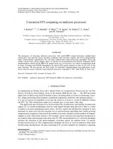
Fig. 19. An iteration of matrix multiplication with the SUMMA algorithm. The number of processes is P = 16 in a grid layout. The matrix size is N × N blocks, with N = 24 (elements are not shown). A rectangle of 6 × 6 blocks is assigned to each process. The figure shows the kth iteration in the execution of the algorithm. Processes with blocks in the kth column of matrix A (P1 , P5 , P9 and P13 in the example) and the kth row of matrix B (P4 , P5 , P6 and P7 in the example) broadcast their blocks to the processes in the same row and column of the grid respectively. As kth column and row in matrices A and B traverse the matrices from k = 0 to N − 1, they are called pivot block column (pbc) and pivot block row (pbr) respectively. The arrows show the particular case of the broadcasting of blocks from the process P5 to those in the same row of the grid in matrix A, and the broadcasting of blocks from the process P6 to those in the same column of the grid in the matrix B.

run a set of kernels by repeating two stages: computation and communication. A kernel is a representative piece of code inside the application such as matrix multiplication or Fourier transform. As a case of study, LogGPH, mlogn P and τ -Lop are used to predict the communication cost of a matrix multiplication kernel for a given layout of the processes on the Tesla multi-core cluster platform. The Scalable Universal Matrix Multiplication Algorithm (SUMMA) [44] is a state-of-the-art computational kernel which is present in many scientific applications. It can be found, for example, in the numerical linear algebra ScaLAPACK library. In this study, we use it as a prototype of other kernels widely used in HPC. In our experimental environment, the distribution of the kernel computational workload is homogeneous. Nevertheless, the difference in performance of the communication channels in the multi-core cluster, the collective communication algorithms and a small but perceptible variation in performance of the processors introduce some imbalances. These imbalances may prevent the processes of the application from the simultaneous arrival at the communication stage, which is typically assumed by any predictive communication model. To reduce the unevenness, we use the FuPerMod [45,46] utility to balance the workload of the application. FuPerMod is a software tool that carries out the whole procedure of the workload partitioning and distribution for a set of processes. It is based on the Functional Performance Model (FPM), which represents the speed of the process by a function of task size. Specifically, we use FuPerMod for 2D partitioning of the matrices involved in the SUMMA algorithm. First, FuPerMod builds the perprocess Functional Performance Model executing a benchmarking code3 provided by the user. Then, using the functional performance models FuPerMod partitions the matrices into sub-matrices and maps the sub-matrices to the processes so that their workload is balanced and the total volume of data communicated between the processes was minimized [47]. In addition, we put a barrier before the communication stage of the application. 5.1. The SUMMA algorithm: a matrix multiplication kernel The SUMMA algorithm computes the dense matrix multiplication C = A × B. The elements of the matrices are grouped in blocks of size b × b elements, making a block the unit of both computation and communication. The granularity of the block size is adjusted prior to multiplication. For simplicity, square matrices are assumed, of the size of N × N blocks. Fig. 19 shows an example for

3 The FPM reflects the speed of a process in executing a particular kernel, thus the benchmarking code has to be as similar to the kernel code as possible.

P = 16 processes arranged in a grid and N = 24 blocks. Each process is assigned a rectangle of the same size (6 × 6 blocks of each matrix) because processors in the system are homogeneous. This mapping balances the computational load, and also minimizes the total volume of data communicated between the processes. The SUMMA algorithm executes in N iterations. A column of blocks and a row of blocks traverse the matrices A and B respectively with each iteration, from k = 0 to N − 1 (see Fig. 19). They are called the pivot block column (pbc) and pivot block row (pbr). In the iteration k, each process computes partial results for all of its assigned blocks of the matrix C . That is, the process owning the block ci j computes ci j = ci j + ai k × bk j . As a consequence, the process has to receive the block in the kth column of the matrix A (ai k ) and the block in the kth row of the matrix B (bk j ). After N

 N −1

iterations, each block will have the value ci j = Thus, each iteration k is composed of three stages:

k=0

ai k × b k j .

1. The processes owning the kth pivot block column (pbc) of the matrix A send the blocks to the processes in the same row (see Fig. 19). In MPI terms, a broadcast operation on a perrow communicator can be used for the communication. The processes owning the blocks in the pbc are the roots of the broadcasts in each row. 2. The processes owning the kth pivot block row (pbr) of the matrix B send the blocks to the processes in the same column (see Fig. 19). In MPI terms, a broadcast operation on a percolumn communicator can be used for the communication. The processes owning the blocks in the pbr are the roots of the broadcasts in each column. 3. Each process Pi updates the blocks in its assigned rectangle of the matrix C . 5.2. Modeling in the Tesla cluster The communication cost of the SUMMA algorithm is evaluated in the Tesla multi-core cluster (see Section 6.1), for both Ethernet and Infiniband networks separately, using the Open MPI library. Open MPI promotes a software architecture based on components. A component is a standalone collection of code that can be inserted into the Open MPI code base, either at run-time and/or compile-time. Tuned component implements collectives similarly to MPICH, as a sequence of point-to-point transmissions between the involved processes. For instance, the RDA algorithm is implemented identically to that in MPICH. Its cost model in the case of Tuned/Ethernet will be given by expressions (16)–(19). However, in the case of Tuned/Infiniband, Open MPI makes use of the RDMA capability of the network, which has an impact in the modeling. A network point-to-point transmission is not modeled

76

J.-A. Rico-Gallego et al. / Future Generation Computer Systems 61 (2016) 66–82

Fig. 22. Process grid for P = 64 and sequential mapping. Number of nodes is M = 8 and number of processes per node is Q = 8. Fig. 20. Mean proportional error of the Recursive Doubling for increasing number of processes deployed on increasing number of nodes with Q = 8. Platform is Tesla with Infiniband and Sequential mapping.

using sequential mapping as Fig. 22 shows. As a consequence of the sequential mapping, broadcasting between processes in the same row of the grid progresses through shared memory, while broadcasting between processes in the same column progresses through the network.6 In a matrix of size N × N, the pbc and pbr have a size of N blocks. Given the process layout of Fig. 22, each process in a row of the grid broadcasts N /M blocks of the pbc. As the size of a block is b2 double precision elements, the size in bytes of the message to broadcast in a row is m=

N M

× b2 × 8 = N b2 = 4096 N .

(21)

Likewise, each process in a column of the grid broadcasts N /Q blocks of the pbr. The value of m does not change because M = Q in Tesla. In LogGPH, the cost of a shared memory row broadcasting, by virtue of (8), is given by: Fig. 21. Mean proportional error of the Recursive Doubling for increasing number of processes deployed on increasing number of nodes with Q = 8. Platform is Tesla with Infiniband and Round Robin mapping.

pbc

0 Tbin (m) = log2 Q × Tp2p (m).

(22)

The cost of broadcasting a column through the network is: by including shared memory transfers to and from the HCA,4 but rather as a single transfer made by the HCA from the sender buffer to the receiver buffer. The cost of a point-to-point transmission defined in (7) is then used to estimate the cost of the RDA algorithm 1 1 in definition (19), with Texch = Tp2p = o1 (m) + L1 (m, 1). The proportional errors of the RDA cost estimations under the Sequential and Round Robin5 mappings on an Infiniband network are shown in Figs. 20 and 21 respectively. Regarding Ethernet, the mean proportional error in the cost estimation of the RDA algorithm for the LogGPH, mlogn P and τ -Lop and P = 64 processes raises respectively to 24.08, 4.35 and 2.80 for sequential mapping and 22.52, 18.41 and 2.60 for round robin mapping. 5.3. Modeling the SUMMA matrix multiplication in the Tesla cluster In this section, we model the communication cost of the SUMMA algorithm in the Tesla platform using LogGPH, mlogn P and τ -Lop. The Open MPI Tuned component provides the implementation of the MPI_Bcast binomial tree algorithm. It is used for the row and column broadcasts in each iteration of the algorithm, as described in Section 5.1. The number of processes is P = 64 arranged in a grid of M × Q , with M = Q = 8,

4 Host Channel Adapter is the name for a network interface card in Infiniband networks. 5 Round Robin mapping places a rank p in the node p%M.

pbr

1 Tbin (m) = log2 M × Tp2p (m).

(23)

In Tesla log2 Q = log2 M = log2 8 = 3, so that the total cost of the SUMMA algorithm under LogGPH is: LogGPH



pbc

pbr



TSUMMA (m) = N × Tbin (m) + Tbin (m)

 0  1 = N × 3 Tp2p (m) + 3 Tp2p (m) = 3 N (L0 + 2 o0 + L1 + 2 o1 ) + 3 N (m − 1) (G0 + G1 ).

(24)

The LogGPH representation of the cost in (24) is independent of the network type, although parameters in the network communication channel have different values for Ethernet and Infiniband (see Section 6.2). In mlogn P the cost is modeled similarly to LogGPH, as defined in (9). The row broadcasting cost is: pbc

Tbin (m) = log2 Q × omw .

(25)

And the cost for the column broadcasting is: pbr

Tbin (m) = log2 M × o′mw + o′net ,





(26)

6 Round robin mapping will use the opposite channel for row and column broadcasts, with identical total cost for the algorithm.

J.-A. Rico-Gallego et al. / Future Generation Computer Systems 61 (2016) 66–82

77

with different values for o′mw and o′net for Ethernet and Infiniband. Thus, according to mlogn P the total communication cost of the algorithm is: mlog P

n TSUMMA (m) = 3 N × omw + o′mw + o′net .





(27)

τ -Lop departs from definition (10) to model the pbc and pbr communications. For the pbc in matrix A, a broadcast per row of the grid of processes in Fig. 22 is executed. Broadcasts in different rows are executed inside different nodes, and hence, they do not contend. Q = 8 processes are involved in each row broadcast, with SEQ Ci = 2i (see definition (10)), with a cost of: pbc

Θbin (m) =

⌈log2 (Q )⌉−1



0 2i ∥ Tp2p (m)



i =0

=

0 Tp2p

0 0 (m) + 2 ∥ Tp2p (m) + 4 ∥ Tp2p (m).

(28)

For the pbr in matrix B, a broadcast per column of the grid of processes is executed. Let us discuss the cost of an individual broadcast in a column of the grid. All the ranks involved in the broadcast are in different nodes. Each point-to-point transmission composing the binomial tree arrives to a different node, and hence, SEQ they do not contend, as set in Section 3.2. As a consequence, Ci = 1 1 in definition (10), and the cost is 3 × Tp2p (m) for M = 8 processes in a column. Bringing together the Q concurrent broadcasts, one per column, the cost including contention is: pbr

Θbin (m) = Q ∥

⌈log2 (M )⌉−1 

SEQ

Ci

Fig. 23. Proportional error in the estimation of the communication cost of the execution of the SUMMA algorithm on the Tesla platform using its 1-Gbit Ethernet network. The size of matrices (N) is given in b×b blocks of double precision elements, b = 64. The number of processes is P = 64 arranged in a grid of 8×8 with sequential mapping.

 1 ∥ Tp2p (m)

i=0

=8 ∥

⌈log2 (M )⌉−1

1 Tp2p (m)

i =0

    1 1 = 8 ∥ 3 × Tp2p (m) = 3 × 8 ∥ Tp2p (m) .

(29)

The total communication cost of the SUMMA algorithm under

τ -Lop is the addition of (28) and (29):  0 τ -Lop 0 0 ΘSUMMA (m) = N × Tp2p (m) + 2 ∥ Tp2p (m) + 4 ∥ Tp2p (m)   1 + 3 × 8 ∥ Tp2p (m) .

(30)

Departing from (30), τ -Lop provides a different representation of the cost for Ethernet and Infiniband networks, following the 1 point-to-point definitions in (6) and (7) respectively for Tp2p (m). The total communication cost of the algorithm in an Ethernet network is:

 τ -Lop ΘSUMMA (m) = N × 3 o0 (m) + 2 L0 (m, 1) + 2 L0 (m, 2) + 2 L0 (m, 4) + 3 o1 (m) + 6 L0 (m, 8)  + 3 L1 (m, 8) , ΘSUMMA (m) = N × 3 o0 (m) + 2L0 (m, 1) + 2L0 (m, 2)  + 2L0 (m, 4) + 3 o1 (m) + 3 L1 (m, 8) .

As a conclusion, the modeling of the communication cost of such a simple but widely used application as matrix multiplication requires to take into account the contention. τ -Lop sets a Q contention factor for the network communication, while LogGPH and mlogn P costs are independent of the number of processes per node. Also, different communication mechanisms of each type of network, such as RDMA in Infiniband, have to be taken into account to achieve a good accuracy in the cost estimation.

(31) 6. Measuring parameters

while in a Infiniband network the cost is modeled as: τ -Lop

Fig. 24. Proportional error in the estimation of the communication cost of the execution of the SUMMA algorithm on the Tesla platform using its QDR Infiniband network. The size of matrices (N) is given in b×b blocks of double precision elements, b = 64. The number of processes is P = 64 arranged in a grid of 8×8 with sequential mapping.



(32)

Fig. 23 shows the mean proportional error in the estimation of the communication cost of the execution of the SUMMA algorithm on the Tesla platform using its Ethernet network. In this case, predictions are given by formulas (24), (27) and (31). Fig. 24 shows the proportional error for the Infiniband network when predictions are given by formulas (24), (27) and (32). The figures demonstrate that τ -Lop error is smaller than the LogGPH and mlogn P ones. Furthermore and more importantly, in the models that do not take into account the contention, the proportional error increases with the growth of problem size N, whereas the cost predicted by τ -Lop approaches the real cost.

An analytical model represents the cost of collective algorithms as a function of the parameters of the model. Therefore, a correct measurement of the parameters is key to achieve accurate predictions. Ensuring the contention of τ processes in the estimation of the transfer time Lc (m, τ ) parameter is the most complex issue in τ -Lop. The authors’ approach is divided in two parts. First, the transfer time in shared memory L0 is estimated, then it is used to figure out the network transfer time L1 from a network point-to-point transmission according to (6). This paper only considers contiguous messages. Therefore, the local costs associated with packing/unpacking of non-contiguous messages are not discussed. Following, an exhaustive methodology for estimating values of the parameters of τ -Lop is presented, together with the

78

J.-A. Rico-Gallego et al. / Future Generation Computer Systems 61 (2016) 66–82

methodology proposed in [26] for LogGPH, and in [34] for mlogn P. Before, the multi-core clusters used as testing platforms are presented. 6.1. The test platforms The experimental platforms used in this paper are Metropolis and Tesla, which include different network technologies and MPI libraries. Metropolis It consists of four nodes connected by 10 Gigabit Ethernet Intel 82574L adapters through a 10 GbE switch Dell PowerConnect 8024F. Each node has two 2.4 GHz Intel Xeon E5620 processors, making a total of eight cores per node, hyperthreading disabled. The cache figures are 12 MB of shared L3, 256 KB of L2 and 32 KB of Harvard L1. The operating system is Linux 2.6.32. The MPI library is MPICH, version 1.4.1p1. This platform is used to evaluate the cost of MPI collective operations. Tesla It is a multi-core cluster equipped with 8 nodes. Each node has two quad-core Intel Xeon E5520 processors running at 2.26 GHz, making a total of eight cores per node. Nodes are connected by a QDR Infiniband (40 Gbps) and an Ethernet (1-GBit) networks. Operating system is CentOS 6.5. The Intel MKL library dgemm function is used to compute a rectangle of double precision elements in the SUMMA algorithm. Open MPI version 1.8.1 [48] is used for communicating the processes in the application. This platform is mainly used for evaluating the cost of the matrix multiplication kernel. IMB (Intel MPI Benchmark) version 3.2 [49] is used to obtain the completion time and bandwidth data. IMB runs on MPICH and Open MPI, the libraries that provide the collective algorithms. The flag of IMB turning cache reuse is deactivated in the command line, forcing data to reach main memory in transfers to avoid cache effects. Measurements of a collective are based on a high number of executions. Each observation is the interval of time from the beginning of the collective to the moment when the last process ends its execution. 6.2. LogGPH and mlogn p For estimating the parameters of the LogGPH model we follow the widely used procedure described by Kielmann et al. in [26]. First, the MPI LogP Benchmark is used for estimating the values of the parameters of the Parametrized LogP (PLogP) model. PLogP slightly changes the meaning of some parameters of LogGP, and makes them (except latency) dependent on the message size. The cost of a point-to-point transmission modeled under PLogP is Tp2p = L + g (m), with L the end-to-end latency from process to process, and g (m) the gap per message, i.e. the minimum time interval between consecutive message transmissions. After that, a simple conversion table (provided in [26]) from PLogP to LogGPH parameter values is applied. The MPI PLogP benchmark provides with two methods of measuring the gap per message: direct and optimized, described in [26]. The direct method is expensive because of the high number of messages used. The optimized method is based on sending only one message, but it has been demonstrated as highly inaccurate by Lastovetsky and Dongarra [50]. In the direct method, Round Trip Time (RTT) of sets of increasing number of messages is measured until the change in g (m) is under 1%, when channel saturation is assumed to be reached. The saturation of the channel makes the network latency negligible with respect to the bandwidth. If the set of n messages sent for a size m has a completion time of sn (m), then the gap per message is calculated as g (m) = sn (m)/n. Tables 1 and 2 show the LogGPH parameters yielded for shared memory and network channels in Metropolis and Tesla platforms respectively. Times are provided in µsecs.

Table 1 LogGPH parameter values (µsecs) in Metropolis cluster. Parameter

Shared memory

Ethernet

L o g G

1.683 0.1095 1.649 0.0001923

32.986 2.8775 4.841 0.0092

Table 2 LogGPH parameter values (µsecs) in Tesla cluster. Parameter

Shared memory

Ethernet

Infiniband

L o g G

0.50 0.20 0.34 0.0003044

24.69 4.40 3.681 0.004289

1.09 0.28 0.60 0.0005589

Regarding mlogn P, according to its authors’ instructions in [34], the Parametrized Round Trip Time (PRTT) defined in [51] is used to measure the o′net time for a range of message sizes. The PRTT (n,d,m) time for a set of n messages sent, a delay of d between message transmissions and the size of message m, is used to calculate the network overhead as: PRTT (n, 0, m) = 2 × o′net . Then, standard blocking MPI_Send and MPI_Recv are used to measure the Round Trip Time in shared memory (RTTshm ) and network (RTTnet ), and to infer omw and o′mw as: RTTshm (m) = 2 × omw =⇒ omw =

RTTshm (m) 2

RTTnet (m) = 2 × omw + onet =⇒ omw =



′

′



′

RTTnet (m) 2

− o′net .

6.3. τ -Lop overhead oc (m) is the time elapsed from the invocation of the operation until the effective data transmission starts through the channel c. The overhead time is assumed not be affected by the contention in the channels. It includes the software stack and protocol times. Most MPI libraries implement two protocols for message passing, with an important impact in the overhead value. They are called eager and rendezvous and perform regardless of the communication channel. They are used for short and large messages respectively. When the message size reaches a threshold size H, the send primitive switches from eager to rendezvous. The value of H is implementation dependent. For instance, in MPICH the Ethernet/TCP network protocol default threshold is H = 128 KB. The protocols work as follows. Eager requires no handshake between sender and receiver, hence data is sent as soon as possible. In the rendezvous protocol, before the data transmission starts, the sender process sends a RTS (Request to Send) message to the receiver, which responds with a CTS (Clear to Send) acknowledgment message when ready to receive. Waiting for this notification avoids the sender to flood the receiver. Our goal is to estimate the overhead in the shared memory and network channels taking into account that it depends on the protocol used. In practice, libraries such as MPICH and Open MPI do not provide noticeable difference in the overhead value in shared memory whatever be the message size. The reason is that they have a common communication mechanism for the whole range of message sizes. The two operations shown in Fig. 25 are used to measure the overhead parameter. Both operations are applicable to MPICH and Open MPI libraries. In both operations, messages of size m = 0 are used, hence with a transfer cost of Lc (0, 1) = 0.

J.-A. Rico-Gallego et al. / Future Generation Computer Systems 61 (2016) 66–82

79

When m < S, no segmentation takes place and the operation cost will be: Ringτ0 (m) = o0 (m) + 2 L0 (m, τ ) ⇒ L0 (m, τ ) =

Ringτ0 (m) − o0 (m)

(35)

.

2 When m ≥ S, messages are segmented and sent as a sequence of k segments of size S, with k = m/S. Every process sends k segments and in turn receives k segments, so the cost will be: Ringτ0 (m) = o0 (m) + 2 k L0 (S , τ ) ⇒ Fig. 25. RTT and Ping operations to measure the overhead o (m) parameter under eager and rendezvous communication protocols respectively. Both operations can be used in shared memory and network communication channels, although, in practice, in shared memory the eager protocol is used exclusively. c

c

c

The first operation is RTT c , shown at the left side of the Fig. 25. It is used to estimate the shared memory overhead o0 (m) for the whole range of messages, and the network overhead o1 (m) under the eager protocol. τ -Lop models the cost of the RTT c operation using a Round Trip message composed of two point-to-point message transmissions. The cost of each message transmission is the addition of the overhead and the sequence of s transfers to reach the destination, as defined in (1). The cost of the operation is:

 RTT (0) = 2 × o (m) + c

c

s−1 

 Lcj

(0, 1) ⇒ oc (m)

j =0

=

RTT c (0) 2

.

(33)

Ringτ0 (m) − o0 (m)

(36)

.

2k The default size for a segment is S = 32 KB both in MPICH and Open MPI. 6.5. τ -Lop network transfer time (L1 )

As discussed in Section 3, communication between processes through the TCP/Ethernet network requires three intermediate transfers for data to reach the destination buffer. The first and the last of these transfers will progress through shared memory, hence with a cost already estimated in (35) and (36). A Ringτ1 operation is set up to measure the network transfer time L1 . 2 τ processes are mapped in a round robin fashion in two nodes, so that even and odd processes will run in different nodes. Ringτ1 operation has two stages. First, each even processes Pi sends to process Pi+1 a message through the network, and then each even process Pi receives from odd processes Pi−1 , resulting in the following cost: Ringτ1 (m) = 2 · o1 (m) + 2 L0 (m, τ ) + L1 (m, τ ) ⇒



c

The Ping operation, shown at the right side of Fig. 25, is used to estimate the overhead in the network o1 (m) under the rendezvous protocol. The MPI Standard defines the synchronous point-to-point MPI_Ssend primitive, which forces the use of the rendezvous protocol in a network message transmission, leading to a cost of: Ping c (0) = oc (m) +

L0 ( S , τ ) =

s−1 

Lcj (0, 1) ⇒ oc (m) = Ping c (0).

(34)

j =0

A high number of iterations in both operations are executed and the average time is used. RTT c operation is not used for the rendezvous protocol because of the following reason. At the right side of Fig. 25, the RTT c operation would add a second point-to-point response message by the process Pj . However, it can start such response message sending the RTS before the process Pi finishes the reception of the CTS. The overlapping of both messages would lead to a wrong overhead estimation. 6.4. τ -Lop shared memory transfer time (L0 ) In both MPICH and Open MPI, communication between processes in shared memory progresses through shared intermediate buffers, so data needs two transfers to reach the destination buffer. A Ringτ0 operation is defined as the exchange of a message of size m between adjacent processes arranged in a ring of τ processes [9]. MPI_Sendrecv is used to execute the Ring operation. Every call to MPI_Sendrecv by process Pi entails a transmission to process Pi+1 , and a transmission from process Pi−1 , with wraparound, and then a wait operation until both complete. The wait provides a synchronization point between processes in each transmission, which ensures that the τ processes transfer data concurrently.

L1 (m, τ ) =

Ringτ1 (m)



− o1 (m) − 2 L0 (m, τ ).

(37)

2 While the overlap of the copying to the NIC internal buffer and transmission through the network is unavoidable, it is not considered in the cost because of its random behavior. No segmentation mechanism is used neither by MPICH nor by Open MPI for transmissions though a TCP/Ethernet network, so (37) can be applied for the whole range of message sizes m. In the Infiniband network, which uses the RDMA mechanism as defined in (7), the procedure to measure the transfer time L1 is similar to that in Ethernet, resulting in: Ringτ1 (m) = 2 · o1 (m) + L1 (m, τ ) ⇒



L1 (m, τ ) =

Ringτ1 (m) 2



− o1 (m).

(38)

6.6. Improving the accuracy in the L(m, τ ) estimation The discussed Ringτc operation, which is used to measure the L parameter in each communication channel c, provides enough accuracy in modeling the complex collectives studied in this paper, as shown in previous sections. Nevertheless, even higher accuracy in the estimation of Lc can be achieved by applying a linear regression procedure. Besides Ring, it can involve the measurements done for other collectives. The target Lc terms will appear now in more than one equation and the best fitting value can be obtained. Expression (35) Ringτ0 (m) = o0 (m) + 2 L0 (m, τ ) can be put as Ringτ0 (m) − o0 (m) = 2 L0 (m, τ ). Moving τ between 1 and 4, for instance, we will make the method used to determine L0 (m, τ ) respond to the trivial linear system c

80

J.-A. Rico-Gallego et al. / Future Generation Computer Systems 61 (2016) 66–82

  Ringτ =1 (m) − o(m) 2 Ring 0 (m) − o(m)   0 τ =2   = 0 Ringτ0=3 (m) − o(m) 0 Ringτ0=4 (m) − o(m) 

0

0 2 0 0

0 0 2 0

L0 (m, 1) 0  0 L0 (m, 2)  0 L0 (m, 3) 2 L0 (m, 4)





which we express in a vector form as dm − om = Rm lm . Vector dm contains the data obtained after measuring the execution times of the Ringτc (m) operations. The system has P equations and P unknowns, four in this case. Beyond Ringτc (m) operation, we know that the broadcast opera0 tion has a cost of Θbcast (m) = 2 o0 (m)+ 2 L0 (m, 1)+ 2 L0 (m, 2) (see Section 4.1). It is possible to enrich the information provided by the 0 Ring measurements with that by Θbcast (m). Now we can add a new equation to the former system, which will take the following form:



Ringτ0=1 (m) − o(m)





2 Ring 0 (m) − o(m)   0 τ =2    Ringτ0=3 (m) − o(m) = 0   0 Ringτ0=4 (m) − o(m) 0 Θbcast (m) − 2 o(m)

2

0 2 0 0 2

0 0 2 0 0



 0 L0 (m, 1) 0  0  L (m, 2)  0  L0 (m, 3) . 2 L0 (m, 4) 0

The method of ordinary least squares can be used to find an approximate solution to this overdetermined system of P + 1 equations and P unknowns. It is well known that such solution is obtained from the problem of finding the lm which minimizes ∥ (dm − om ) − Rm lm ∥2 . Note that this is just an example. More and different equations can be added to the problem of estimating the parameters of τ -Lop. This methodology is mainly aimed at getting a higher level of accuracy in cost estimation of different applications, by adding the execution time of collectives actually invoked by the applications. This expected overall improvement in modeling the communication costs of applications comes hence at the expense of benchmarking their collectives. 7. Conclusions Current HPC platforms demand better communication performance models able of capturing their growing complexity, in particular the heterogeneity of the communication channels and the increasing number of cores per node. This work addresses the cost modeling of some of the algorithms underlying collective operations present in MPI implementations as MPICH or Open MPI on multi-core platforms. The algorithms discussed, being fairly common, have been chosen because their complexity significantly exceeds that of the algorithms evaluated in previous related works. We analyze algorithms under three performance models in hierarchical platforms. LogGPH extension of the LogGP model is representative of the broadly used linear models which use network-related latency and bandwidth parameters, and estimate the cost of an algorithm as the cost of the longest path of the involved point-to-point transmission. mlogn P, an extension of the logn P model, changes previous view of the point-to-point transmissions modeled using network parameters and introduces a decomposition on transfers through the communication channels hierarchy. Finally, τ -Lop offers a more global view of an algorithm behavior based on the concept of concurrent transfers and a simple but still powerful notation for them. In this paper we have shown that τ -Lop is able to capture the impact of bandwidth shrink in shared channels when several transmissions progress in parallel, with the overall result of improving the accuracy of the cost estimation. In addition, we reveal that overlooking the representation of the contention leads to unacceptable estimation errors. MPI is the de facto standard used by almost all applications running in high performance computing platforms. Modeling and

Fig. 26. Example of the Relative error ρ of two estimated values with respect to their respective real measurements.

estimating the communication cost of these parallel applications reduces to modeling the MPI operations invoked by them. As a case of study, we address the cost estimation of a representative matrix multiplication kernel in a multi-core cluster platform using Ethernet and Infiniband network technologies. As before, the conclusion is that τ -Lop shows a more scalable and accurate cost estimation than LogGPH and mlogn P in both type of networks. Finally, an exhaustive methodology for estimating the τ -Lop parameters is proposed. Acknowledgments This work was supported by the Extremadura Supercomputing Center (CenitS) and by the computing facilities of Extremadura Research Centre for Advanced Technologies (CETA-CIEMAT), funded by the European Regional Development Fund (ERDF). This work has been partially supported by EU under the COST programme Action IC1305, ‘Network for Sustainable Ultrascale Computing (NESUS)’, and by Science Foundation Ireland under Grant Number 14/IA/2474. Appendix. Accuracy of the measurements with the proportional error The utility of a model is determined largely by the accuracy achieved in the estimation of its parameters, which results in the correct prediction of the cost of the operations. Several error metrics exist to express the accuracy of an estimation with respect to the real measurement. Usually, Relative error is used in the literature, based on the distance between estimated and real values. Lets call ρ the Relative error of an estimated value e with respect to the real value r. It is defined [52] as

ρ=

|e − r | r

.

(39)

The concept of relative error as an expression of error suffers an anomaly outlined hereafter. Fig. 26 illustrates this point with an example. The first estimated value is e, with a Relative error with respect to the measured value r of ρ = 1. For the estimated value e′ , the Relative error with respect to r ′ is ρ ′ = 0.5. Therefore, ρ ≫ ρ ′ , even though the distance and proportion among estimated and real values are equal. This fact has an impact in the communication performance modeling evaluation. A model that underestimates the cost of an algorithm will give a lower Relative error than a model that overestimates it in the same proportion. For this reason this paper discards the Relative error and uses an error measurement based on the proportion between real and estimated values, which

J.-A. Rico-Gallego et al. / Future Generation Computer Systems 61 (2016) 66–82

reflects the accuracy of the measures in a more meaningful way. We define the Proportional error µ of a estimated value e with respect to the real value r as:

µ=

max(r , e) min(r , e)

.

(40)

Under the hypothesis that both e and r are positive numbers, the Proportional error is always greater than 1, equal when there is no error. Regarding the example in Fig. 26, Proportional errors will be identical (µ = µ′ = 2) because their predictions fail in the same proportion. The Proportional error is applied to sets of estimated values obtained from different models in order to compare them, and with the real values. Being times, real and estimated values are positive numbers. The procedure is as follows. In starting from two sets of discrete values R and E M , where R represents the measured communication times, and E M represents the estimated values by a model M for an operation: R = {r0 , r1 , r2 , . . . , rn−1 }

(41)

M M M E M = {eM 0 , e1 , e2 , . . . , en−1 }.

That is, ri is the measured value for the message size i, and eM i is the estimated value for the message size i by the model M of an operation. The proportion between the set of measured and estimated values is defined as: M M M µM = {µM 0 , µ1 , µ2 , . . . , µn−1 },

with each component µM i as the Proportional error of the estimated value with respect to the real measurement for the message size i, defined in (40). However, neither the Proportional nor the Relative errors give information about which range of values (R or E M ) is higher, and it needs to be provided in each context. The Average Proportional error of the model M for the whole range of message sizes in the set µM is: n −1

 µ ¯ = M

µM i

i =0

n

.

(42)

There is a simple relation between Relative and Proportional error that allows the conversion from one to the other. Let us consider the Relative error ρ defined in (39) of a single estimated value e with respect to the real value r, and the Proportional error µ defined in (40) for the same pair. We have two cases: e > r and e < r. Note that when e = r no error applies, that is, the Relative error is 0 and the Proportional error is 1. 1. If e > r, then µ = e/r, and then:

ρ=

e−r r

=

(µ r ) − r r

= µ − 1.

(43)

And then:

µ=ρ+1

(44)

2. If e < r, then µ = r /e, and then:

ρ=

r −e r

=

r − (r /µ) r

=1−

1

µ

.

(45)

So that:

µ=

1 1−ρ

.

(46)

81

References [1] MPI Forum. MPI: A Message-Passing Interface Standard. Version 3.0, September 21th 2012. Available at: http://www.mpi-forum.org. [2] Rolf Rabenseifner, Automatic profiling of MPI applications with hardware performance counters, in: Proceedings of the 6th European PVM/MPI Users’ Group Meeting on Recent Advances in Parallel Virtual Machine and Message Passing Interface, Springer-Verlag, London, UK, 1999, pp. 35–42. [3] Roger W. Hockney, The communication challenge for MPP: Intel Paragon and Meiko CS-2, Parallel Comput. 20 (3) (1994) 389–398. [4] David E. Culler, Richard M. Karp, David Patterson, Abhijit Sahay, Eunice E. Santos, Klaus Erik Schauser, Ramesh Subramonian, Thorsten von Eicken, LogP: a practical model of parallel computation, Commun. ACM 39 (1996) 78–85. [5] Fumihiko Ino, Noriyuki Fujimoto, Kenichi Hagihara, LogGPS: a parallel computational model for synchronization analysis, SIGPLAN Not. 36 (2001) 133–142. [6] Liang Yuan, Yunquan Zhang, Yuxin Tang, Li Rao, Xiangzheng Sun, LogGPH: A parallel computational model with hierarchical communication awareness, in: Computational Science and Engineering (CSE), 2010 IEEE 13th International Conference on, 2010, pp. 268–274. [7] Kirk W. Cameron, Rong Ge, Predicting and evaluating distributed communication performance, in: Proceedings of the 2004 ACM/IEEE conference on Supercomputing, SC’04, IEEE Computer Society, Washington, DC, USA, 2004, p. 43. [8] K.W. Cameron, R. Ge, X.H. Sun, logm p and log3 p: Accurate analytical models of point-to-point communication in distributed systems, IEEE Trans. Comput. 56 (3) (2007) 314–327. [9] Juan-Antonio Rico-Gallego, Juan-Carlos Díaz-Martín, τ -Lop: Modeling performance of shared memory MPI, Parallel Comput. 46 (2015) 14–31. [10] Kirk W. Cameron, Xian-He Sun, Quantifying locality effect in data access delay: Memory logP, in: Proceedings of the 17th International Symposium on Parallel and Distributed Processing, IPDPS’03, IEEE Computer Society, Washington, DC, USA, 2003. [11] E.W. Chan, M.F. Heimlich, A. Purkayastha, R.A. van de Geijn, On optimizing collective communication, in: Cluster Computing, 2004 IEEE International Conference on, 2004, pp. 145–155. [12] Rajeev Thakur, Rolf Rabenseifner, William Gropp, Optimization of collective communication operations in MPICH, Int. J. High Perform. Comput. Appl. 19 (1) (2005) 49–66. [13] Albert Alexandrov, Mihai F. Ionescu, Klaus E. Schauser, Chris Scheiman, LogGP: incorporating long messages into the logp model—one step closer towards a realistic model for parallel computation, in: Proc. of the Seventh Annual ACM Symposium on Parallel Algorithms and Architectures, SPAA’95, NY, USA, 1995, pp. 95–105. [14] Csaba Andras Moritz, Matthew I. Frank, LoGPC: Modeling network contention in message-passing programs, IEEE Trans. Parallel Distrib. Syst. 12 (4) (2001) 404–415. [15] WenGuang Chen, JiDong Zhai, Jin Zhang, WeiMin Zheng, LogGPO: An accurate communication model for performance prediction of MPI programs, 52 (10) (2009) 1785–1791. [16] Khalid Al-Tawil, Csaba Andras Mortíz, Performance modeling and evaluation of MPI, J. Parallel Distrib. Comput. 61 (2) (2001) 202–223. [17] Jelena Pješivac-Grbović, Thara Angskun, George Bosilca, Graham E. Fagg, Edgar Gabriel, Jack J. Dongarra, Performance analysis of MPI collective operations, Cluster Comput. 10 (2007) 127–143. [18] Ernie Chan, Marcel Heimlich, Avi Purkayastha, Robert van de Geijn, Collective communication: Theory, practice, and experience: Research articles, Concurr. Comput.: Pract. Exper. 19 (13) (2007) 1749–1783. [19] Rajeev Thakur, WilliamD. Gropp, Improving the performance of collective operations in MPICH, in: Recent Advances in Parallel Virtual Machine and Message Passing Interface, in: Lecture Notes in Computer Science, vol. 2840, Springer, Berlin Heidelberg, 2003, pp. 257–267. [20] Jesper Larsson Träff, Andreas Ripke, An Optimal Broadcast Algorithm Adapted to SMP Clusters, in: Lecture Notes in Computer Science, vol. 3666, Springer, Berlin Heidelberg, 2005, pp. 48–56. [21] Prashanth B. Bhat, C.S. Raghavendra, Viktor K. Prasanna, Efficient collective communication in distributed heterogeneous systems, J. Parallel Distrib. Comput. 63 (3) (2003) 251–263. [22] J. Hatta, S. Shibusawa, Scheduling algorithms for efficient gather operations in distributed heterogeneous systems, in: Parallel Processing, 2000. Proceedings. 2000 International Workshops on, 2000, pp. 173–180. [23] F. Ooshita, S. Matsumae, T. Masuzawa, Efficient gather operation in heterogeneous cluster systems, in: High Performance Computing Systems and Applications, 2002. Proceedings. 16th Annual International Symposium on, 2002, pp. 196–204. [24] Rolf Rabenseifner, JesperLarsson Träff, More efficient reduction algorithms for non-power-of-two number of processors in message-passing parallel systems, in: Lecture Notes in Computer Science, Vol. 3241, Springer, Berlin, Heidelberg, 2004, pp. 36–46. [25] L.V. Kale, S. Kumar, K. Varadarajan, A framework for collective personalized communication, in: Parallel and Distributed Processing Symposium, 2003. Proceedings. International, 2003, p. 9. [26] Thilo Kielmann, Henri E. Bal, Kees Verstoep, Fast measurement of logP parameters for message passing platforms, in: Proceedings of the 15 IPDPS 2000 Workshops on Parallel and Distributed Processing, IPDPS’00, SpringerVerlag, London, UK, 2000, pp. 1176–1183.

82

J.-A. Rico-Gallego et al. / Future Generation Computer Systems 61 (2016) 66–82

[27] Luiz Angelo Barchet-Estefanel, Grégory Mounié, Identifying logical homogeneous clusters for efficient wide-area communications, in: Lecture Notes in Computer Science, Vol. 3241, Springer, Berlin, Heidelberg, 2004, pp. 28–35. [28] Alexey Lastovetsky, Vladimir Rychkov, Accurate and efficient estimation of parameters of heterogeneous communication performance models, Int. J. High Perform. Comput. Appl. 23 (2) (2009) 123–139. [29] A. Lastovetsky, V. Rychkov, M. O’Flynn, Revisiting communication performance models for computational clusters, in: Parallel Distributed Processing, 2009. IPDPS 2009. IEEE International Symposium on, 2009, pp. 1–11. [30] T. Hoefler, T. Mehlan, F. Mietke, Wolfgang Rehm, Logfp—a model for small messages in infiniband, in: Parallel and Distributed Processing Symposium, 2006. IPDPS 2006. 20th International, 2006, p. 6. [31] T. Hoefler, T. Schneider, A. Lumsdaine, Multistage switches are not crossbars: Effects of static routing in high-performance networks, in: Cluster Computing, 2008 IEEE International Conference on, 2008, pp. 116–125. [32] Sang Cheol Kim, Sunggu Lee, Measurement and prediction of communication delays in myrinet networks, J. Parallel Distrib. Comput. 61 (11) (2001) 1692–1704. [33] A. Lastovetsky, I.-H. Mkwawa, M. O’Flynn, An accurate communication model of a heterogeneous cluster based on a switch-enabled ethernet network, in: Parallel and Distributed Systems, 2006. ICPADS 2006. 12th International Conference on, Vol. 2, 2006, pp. 15–20. [34] Bibo Tu, Jianping Fan, Jianfeng Zhan, Xiaofang Zhao, Performance analysis and optimization of MPI collective operations on multi-core clusters, J. Supercomput. 60 (1) (2012) 141–162. [35] Maxime Martinasso, Jean-François Méhaut, A contention-aware performance model for hpc-based networks: a case study of the infiniband network, in: Proceedings of the 17th International Conference on Parallel Processing— Volume Part I, Euro-Par’11, Springer-Verlag, Berlin, Heidelberg, 2011, pp. 91–102. [36] Maxime Martinasso, Jean-François Méhaut, Prediction of communication latency over complex network behaviors on SMP clusters, in: Lecture Notes in Computer Science, Vol. 3670, Springer, Berlin, Heidelberg, 2005, pp. 172–186. [37] V. Jerome, M. Maxime, V. Jean-Marc, M. Jean-Francois, Predictive models for bandwidth sharing in high performance clusters, in: Cluster Computing, 2008 IEEE International Conference on, 2008, pp. 286–291. [38] Jun Zhu, Alexey Lastovetsky, Shoukat Ali, Rolf Riesen, Communication models for resource constrained hierarchical ethernet networks, in: 11th International Workshop on Algorithms, Models and Tools for Parallel Computing on Heterogeneous Platforms (HeteroPar’2013), Aachen, Germany, 2013. 26 August. [39] L.A. Steffenel, Modeling network contention effects on all-to-all operations, in: Cluster Computing, 2006 IEEE International Conference on, 2006, pp. 1–10. [40] Juan-Antonio Rico-Gallego, Juan-Carlos. Díaz-Martín, Alexey L. Lastovetsky, Modeling contention and mapping effects in multi-core clusters, in: Sascha Hunold, et al. (Eds.), Euro-Par 2015: Parallel Processing Workshops, in: Lecture Notes in Computer Science, Vol. 9523, Springer International Publishing, 2015, pp. 197–208. [41] Brice Goglin, Stéphanie Moreaud, KNEM: a generic and scalable kernelassisted intra-node MPI communication framework, J. Parallel Distrib. Comput. 73 (2) (2013) 176–188. [42] Hyun wook Jin, Sayantan Sur, Lei Chai, Dhabaleswar K. Panda, Limic: Support for high-performance mpi intra-node communication on linux cluster, in: In International Conference on Parallel Processing (ICPP), 2005, pp. 184–191. [43] Jiuxing Liu, Jiesheng Wu, Sushmitha P. Kini, Pete Wyckoff, Dhabaleswar K. Panda, High performance RDMA-based MPI implementation over infiniband, in: Proceedings of the 17th Annual International Conference on Supercomputing, ICS’03, ACM, New York, NY, USA, 2003, pp. 295–304. [44] R.A. van de Geijn, J. Watts, SUMMA: Scalable Universal Matrix Multiplication Algorithm, Tech. Rep., Austin, TX, USA, 1995. [45] D. Clarke, Z. Zhong, V. Rychkov, A. Lastovetsky, FuPerMod: A framework for optimal data partitioning for parallel scientific applications on dedicated heterogeneous HPC platforms, in: 12th International Conference on Parallel Computing Technologies (PaCT-2013), in: Lecture Notes in Computer Science, vol. 7979, Springer, Russia, 2013, pp. 182–196. [46] D. Clarke, Z. Zhong, V. Rychkov, A. Lastovetsky, FuPerMod: a software tool for the optimization of data-parallel applications on heterogeneous platforms, J. Supercomput. 69 (2014) 61–69.

[47] A. Lastovetsky, R. Reddy, Data partitioning with a functional performance model of heterogeneous processors, Int. J. High Perform. Comput. Appl. 21 (1) (2007) 76–90. [48] D. Kranzlmüller, P. Kacsuk, J. Dongarra, E. Gabriel, G. Fagg, G. Bosilca, T. Angskun, J. Dongarra, J. Squyres, V. Sahay, P. Kambadur, B. Barrett, A. Lumsdaine, R. Castain, D. Daniel, R. Graham, T. Woodall, Open MPI: Goals, concept, and design of a next generation MPI implementation, in: Lecture Notes in Computer Science, Vol. 3241, Springer, Berlin, Heidelberg, 2004, pp. 97–104. [49] Intel. Intel MPI benchmarks. Available at: https://software.intel.com/enus/articles/intel-mpi-benchmarks. Last checked: 2015, Sept. 22th. [50] J. Dongarra, A.L. Lastovetsky, High Performance Heterogeneous Computing, Wiley-Interscience, New York, NY, USA, 2009. [51] Torsten Hoefler, Torsten Mehlan, Andrew Lumsdaine, Wolfgang Rehm, Netgauge: A network performance measurement framework, in: Lecture Notes in Computer Science, Vol. 4782, Springer, Berlin, Heidelberg, 2007, pp. 659–671. [52] M. Abramowitz, I.A. Stegun, Handbook of mathematical functions with formulas, graphs, and mathematical tables, in: National Bureau of Standards Applied Mathematics Series, Vol. 55, U.S. Government Printing Office, Washington, D.C, 1964. For sale by the Superintendent of Documents.

Juan Antonio Rico Gallego received the Computer Science Engineering from the University of Extremadura in 2002. Formerly a software consultant, he is an associate professor at the Department of Computer Systems Engineering and Telematics of the University of Extremadura (Spain), where he teaches foundation and concurrent programming. He is pursuing the Ph.D. degree in Computer Science on MPI and OpenMP performance models. Other research interest include MPI implementation and current trends and issues concerning Exascale software. He codevelops and maintains AzequiaMPI, an efficient thread-based fully MPI 1.3 standard implementation.

Juan Carlos Díaz Martín received the Computer Science Engineering and the Ph.D. degree in Computer Science from the Polytechnique University of Madrid, in 1988 and 1993 respectively. He is currently an Associate Professor at the Department of Computer and Communication Technology of University of Extremadura in Cáceres (Spain), where he teaches distributed and multicore programming, real-time systems and operating system design. His research interest is in MPI implementation and applications. He codevelops and maintains AzequiaMPI, an efficient thread-based fully MPI 1.3 standard implementation. He has also carried out work in High Performance Reconfigurable Computing, producing MPI implementations for commercial distributed platforms of digital signal processing as well as for soft-core processors in networked FPGA’s. Finally, he deals with the problem of finding the roots of arbitrarily high degree polynomials through parallel geometric methods.

Alexey Lastovetsky received a Ph.D. degree from the Moscow Aviation Institute in 1986, and a Doctor of Science degree from the Russian Academy of Sciences in 1997. His main research interests include algorithms, models, and programming tools for high performance heterogeneous computing. He has published over a hundred technical papers in refereed journals, edited books, and international conferences. He authored the monographs Parallel computing on heterogeneous networks (Wiley, 2003) and High performance heterogeneous computing (Wiley, 2009).