from PCM by (modulo-2) Gaussian elimination. The method is the same for any block code, thus it does not deploy the sparseness of LDPC codes, and the ...
Low-Complexity Encoding of LDPC Codes: A New Algorithm and its Performance Hanghang Qi and Norbert Goertz Institute for Digital Communications Joint Research Institute for Signal & Image Processing School of Engineering and Electronics The University of Edinburgh Mayfield Rd., Edinburgh EH9 3JL, Scotland, UK Email: {H.Qi, Norbert.Goertz}@ed.ac.uk Abstract— A new technique for efficient encoding of LDPC codes based on the known concept of approximate lower triangulation (ALT) is introduced. The greedy permutation algorithm is presented to transform parity-check matrices into an approximate lower triangular (ALT) form with minimum “gap”. A large girth, which is known to guarantee good decoding performance, is shown (for a fixed column-weight of the parity-check matrix of the code) to result in a large gap to linear encoding, which demonstrates a fundamental trade-off between complexity and decoding performance.
I. I NTRODUCTION Low-density parity-check (LDPC) codes [1] can, for large blocksize, achieve a performance very close to the Shannon limit [2], with low-complexity iterative decoding by “Believe Propagation” (BP) or the Sum-Product Algorithm (SPA) [3]. Decoding of LDPC codes can be performed efficiently as long as the parity-check matrices are sparsely populated with “ones”. The “girth”, which is the length of the shortest cycle in the Tanner graph [4] of the code, determines the performance under BP decoding. The sparseness of the parity-check matrix (PCM) allows for decoding with low complexity based on a graph based decoder. However, encoding with low complexity is not straightforward, as LDPC codes are defined by their PCM and the generator matrix is generally unknown. The conventional way is systematic encoding [3] with the generator matrix derived from PCM by (modulo-2) Gaussian elimination. The method is the same for any block code, thus it does not deploy the sparseness of LDPC codes, and the complexity is O(n2 ) (Preprocessing O(n3 ), actual encoding by matrix mulitplication O(n2 )) where n is the length of the codewords; for large blocksize n the encoding complexity can be significant. Some novel ideas for lower-complexity LDPC encoding where the spaseness of PCM is exploited have been presented recent years: the graph-based message-passing encoder [5], [6] is a technique that uses the decoder for encoding by assumimg that the unknown parity bits have been erased by the channel. Hence, the encoding process is exactly the same as decoding after transmission over a binary erasure channel (BEC). The idea applies to any LDPC code – regular or irregular, random
or structured. The method, however, does not always work, in particular when stopping sets [7] exist within the code. Another encoding method which applies to any LDPC code and which always works was proposed in [8]. The idea is to transform the PCM into an approximate lower triangular (ALT) form by row and column permutations only (but without any additions of rows!), which preserves the sparseness of the matrix. Then the encoding complexity is O(n + g 2 ), where g is called the “gap” to linear encoding1 . This “gap” is actually the number of rows of the PCM that can not be brought into triangular form by row and column permutations only. Although the concept presented in [8] is convincing, no exact “programmable” step-by-step algorithm is given that describes how to get an ALT form of the PCM that has a small gap: this is exactly the topic of the work presented in this paper. We discuss the gap to “linear encoding” of LDPC codes and we show the tradeoff between the encoding complexity and the performance: the gap must increase when the performance increases. The paper is organized as follows: In Section II the idea of almost linear encoding with the ALT method is reviewed and compared with systematic encoding by Gaussian elimination. In Section III we present our novel “greedy permutation” algorithm to get a “good” ALT form from the PCM with minimum gap g. Numerical results are given in Section IV. II. A LMOST L INEAR E NCODING WITH A PPROXIMATE L OWER T RIANGULATION (ALT) A. Systematic Encoding by Gaussian elimination Firstly, we review the traditional method for encoding a block code with a known PCM: we use Gaussian elimination to find the unknown generator matrix from the PCM. Getting the PCM, H, into systematic form is achieved through row permutations, modulo-2 sums of rows and some column permutations (if neccesary) to make the right part of the PCM a unit matrix I. We obtain H0 = {P, I} from which, by standard 1 By “linear encoding” we mean that the complexity of channel encoding grows linearly with the block size, n, of the channel code. We use the notation “O(n)” to indicate a complexity order with this linear growth.
rules [3], we otbain the generator matrix G = {Ik , PT }. Then, if the information word is u, the channel codeword v is given by v = u · G. From left to right, the information bits are the leading bits in the codeword followed by the parity check bits. In other words, having the PCM, H, in the equivalent systematic form, H0 , we know how the parity check bits are linearly calculated from the information bits. The computational complexity of reducing the PCM, Hm×n , to its systematic form is O(n3 ). And, as the sparseness of H is lost during Gaussian elimination, the complexity of actual encoding is generally that of a matrix multiplication, i.e., encoding has a complexity of order O(n2 ). B. Encoding with a Complexity that Grows Approximately Linear with the Blocksize The parity-check matrix (PCM) of a LDPC code is “sparse” by definition, and, although the generator matrix (GM) is generally not sparse, we would like to perform encoding with low complexity, preferably close to a complexity-order O(n), with n the block size of the code, i.e., we would like the complexity of encoding to grow only linear with n. Encoding by “Approximate Linear Triangulation” (ALT) of the PCM presented in [8] achieves a complexity of O(n+g 2 ), where g is the gap to linear encoding with g � n. The idea is to transform the PCM, H, with as small gap g as possible, into an equivalent2 “almost lower triangular” form, H1 , as illustrated by Fig. 1. As the ALT form, H1 , of the PCM, H, n−m
m−g
g
0
m
A
B
T
m−g
C
D
E
g
n Fig. 1. form.
Parity check matrix, H1 , in approximate lower triangular (ALT)
is obtained by row and column permutations only, the submatrices A, B, C, D, T and E are all sparse matrices. In a second step we keep the matrices A, B and T , and we transform the matrix E into an “all-zero” matrix and the matrix D into an identity matrix, both by Gaussian elimination. The resulting equivalent PCM has “systematic approximate lower triangular” (SALT) form and full rank, and we denote this PCM by HH; it is illustrated by Fig. 2. Note that we assume that during the process of transformation of the original PCM, 2 Equivalent in the sense that all PCMs check the same channel code. Below, however, we will extend the notion of “equivalence” to PCMs that check codes in which some of the code bits are re-ordered although the code is, structurally, still the same.
n−m
g
m−g 0
m
A
B
C1
0
T
m−g
0
g
D1 0
n Fig. 2. Parity Check Matrix, HH, in systematic approximate lower triangular (SALT) form.
H, into the equivalent form, HH, any linear dependent rows (which frequently but not necessarily occur in LDPC code constructions) are removed, so that the equivalent SALT form HH of the PCM has full rank and the number of rows equals the number m of parity bits. To obtain the diagonal structure for the matrix T we may have to permute columns, which means that we relocate bit-positions within the code word. Although this means that the matrices H and HH will not describe exactly the same code, the codewords will only differ in the ordering of the bits. This trivial type of change is assumed to be contained in our notion of “equivalence” of PCMs. Due to the structure of the SALT form (Fig. 2) we can conveniently pick the first n − m bit positions (from the left) in the codeword to be the data bit positions, i.e., the columns corresponding to the matrices A and C1 are those of the data bits. Hence, the codewords have the following structure: v = (u, p1 , p2 ) with u the n − m data bits, p1 the first g parity bits and p2 the remnaining (m − g) parity bits. The first g parity bits p1 can be directly determined from the sub-matrices C1 and D1 according to p1 = u · C1T . Further, from the parity-check condition H · v T = 0n×1 for T any codeword v, we obtain A · uT + B · pT 1 + T · p2 = 0m×1 . As the matrix T has lower triangular form, we obtain the second set p2 = {p2 (1), p2 (2), ..., p2 (m − g)} of parity bits by back-substitution (details are given in [8]): p2 (l) =
n−m X j=1
Al,j · uj +
g X j=1
Bl,j · p1 (j) +
l−1 X
Tl,j · p2 (j) (1)
j=1
for l = 1, 2, ..., m − g (all arithmetic operations “modulo-2”). For a complexity analysis of the encoding procedure described above it is important to realise that, except for the submatrix C1 , all submatrices are still sparse and that D1 is a g × g indentity matrix. There are n − m information bits and m parity check bits. Among them there are m − g linearly encoded parity check bits (those we get from (1) by back-substitution) and g parity bits we get from the matrix multiplication p1 = u · C1T with C1 not sparse. The total complexity of encoding by this method turns out to be of
order O(n + g 2 ); the details of the complexity analysis are given [8]. Note that the gap to linear enoding complexity is determined by the number g of non-sparse rows in the matrix C1 . Therefore, the goal is to find a SALT form of the PCM with g as small a possible: this is, e.g., achieved by the greedy permutation algorithm proposed in the next section. III. G REEDY P ERMUTATION A LGORITHM The key of the encoding method described in Section II-B is to get the SALT form of the PCM with minimum gap g, because the smaller the gap is, the more efficient encoding will be. The problem of finding the SALT form with minimum gap is rather hard, especially when H is large, because the larger the matrix dimensions are, the more possibilities for row and column-permutations exist and it is not straightforward which permutations to use in which order to obtain the best result. Below, we present an algorithm to get the SALT form of the PCM with “small” (but not necessarily the minimum) gap. It applies to any LDPC code and it is efficient for both regular and irregular codes. We call the scheme a “greedy permutation algorithm” and its complexity is O(n3 ), which is the same as Gaussian elimination. We note that in the SALT form of the PCM, the “ones” are concentrated in the left-bottom corner of the PCM (submatrix C1 ). Moreover, in the last m − g columns of the SALT form, all “ones” will lie on or below the matrix main diaogonal (see Fig. 2) of the submatrix T . To obtain this SALT form, we start from the original PCM, H, and work column-wise backwards from column n to column n − m + g + 1. We first find the column 1, ..., n of the original PCM, H, which has the smallest number of “ones”: we place this column at position n (i.e., at the very right-hand side) of the “new” PCM. Then we permute the rows such, that all “ones” in column n appear at the bottom of the new, equivalent PCM. Next, we search all columns to the left of the previously considered one (i.e., columns 1, ...., n − 1 initially) and we place the column with the smallest number of “ones” on and above the main diagonal (see submatrix T in Fig. 2) at position n−1. If there is only one “one” on or above the main diagonal, we permute the row with this “one” in column n−1 to the main diagonal (if it is not there anyway). If there are more than one “ones” in column n − 1, we permute one of the corresponding rows such that the “one” is located on the main diagonal. The other rows with “ones” in column n − 1 are permuted to the bottom of the matrix and the gap g increases exactly by this number of rows. Then we search the columns left of n − 1 again for that one with the smallest number of “ones” on or above the main diagonal of the submatrix T and we proceed as described above, until we reach the first row with the main diagonal of the matrix T : then we have obtained the ALT form of the PCM (see Fig. 1). In the next step we leave the rows 1....m − g unchanged and we use the lower-diagonal matrix T to cancel all “ones” in the sub-matrix E in Fig. 1. After that we use Gaussian elimination to transform the matrix D in Fig. 1 into an g × g
identity matrix: during this process (but also when cancelling the matrix E as described above) we loose the sparsity of C1 . During Gaussian elimination we might encounter linear dependent rows that we remove: this reduces the gap which is, of course, very welcome. The greedy permutation algorithm is summarised in Table I. The computational cost to transform a given PCM to the TABLE I D ESCRIPTION OF THE G REEDY P ERMUTATION A LGORITHM We start with a given PCM with m rows and n columns; there may be redundant rows. Initialisation: search for the column with smallest number k0 > 0 of “ones” (random choice if more than one such column exists). Permute this column to the rightmost position, i.e., to the columnindex n. Permute all k0 rows which have a “one” in the last column to the bottom of the PCM. Set the current gap to g = k0 − 1. The current submatrix T starts at the lower right-hand corner with a “one” in row m − g and column n. Set p = n − 1 and j = 1. Step 1: Search for the index 1, ..., p of the column in which there is the smallest number kj > 0 of “ones” on or above the main diagonal of the current sub-matrix T (arbitrary choice if more than one such column exists). This is the smallest number of “ones” in any column 1, ..., p in the rows 1, ..., m − g + j. Permute the “best” column to column-index p. Is there only one “one” on or above the main diagonal of the sub-matrix T in the column permuted to column-index p? Yes No If the “one” is above the main Pick any row with an index diagonal of T permute the corre1, ..., m−g+j which has a “one” sponding row such that the “one” in column p and permute it to is placed on the main diagonal of row-index m−g +j. Append the the sub-matrix T . This is permute remaining number rj rows with the row with an index 1, ..., m − indices 1, ..., m−g+j+1, which g + j + 1 (which has a “one” in also have a “one” in column p, column “p”) with the row with at the bottom of the PCM. The index m − g + j. gap increases, i.e., the new gap is g := g + rj . Set j := j + 1 and p := p − 1. If m − g − j < 1 GoTo Step 2; otherwise GoTo Step 1. Step 2: ALT-form is obtainted. Convert the ALT into the SALT form: start from the right in Fig. 1 and cancel all “ones” in the submatrix E by adding rows from the submatrix T . Afterwards, perform Gaussian elimination on the matrices C and D to transform D into an identity matrix D1 . The result is the SALT form illustrated by Fig. 2. During Gaussian elimination, some of the g rows at the bottom of the matrix may turn out to be linearly dependent. Remove these rows; the gap g is reduced by the number of linearly dependent rows.
ALT form using greedy permutation algorithm is O(n3 ), and transforming the ALT form to the SALT form takes a complexity of order O(n2 + g 3 ). Hence, the total complexity is O(n3 ), which is the same as Gaussian elimination. This complexity, is however, not critical, as the SALT form needs to be computed only once and “off-line”, before the system is used. The important part is that the SALT form of the matrix allows for efficient encoding by exploiting the sparsity of the original PCM. Example 1: To illustrate the proposed greedy permutation algorithm in Table I, we give a detailed example. Consider the
following PCM taken from [1]:
H=
1 1 . . . . 1 . . . . 1 . . . .
2 1 . . . . . 1 . . . . 1 . . .
3 1 . . . . . . 1 . . . . 1 . .
4 1 . . . . . . . 1 . . . . 1 .
5 . 1 . . . 1 . . . . . . . . 1
6 . 1 . . . . 1 . . . 1 . . . .
7 . 1 . . . . . 1 . . . 1 . . .
8 . 1 . . . . . . . 1 . . 1 . .
9 . . 1 . . 1 . . . . . . . 1 .
10 11 12 13 14 15 16 17 18 19 20 . . . . . . . . . . . . . . . . . . . . . . 1 1 1 . . . . . . . . . . . 1 1 1 1 . . . . . . . . . . . 1 1 1 1 . . . 1 . . . . . . . 1 . . . . . . 1 . . . . . . . 1 . . . 1 . . . 1 . . . 1 . . . 1 . . . 1 . . . 1 . . . 1 . . 1 . . . . . 1 . . . 1 . . . . 1 . . . . . . . 1 . . . . . 1 . . . . . 1 . . 1 . . . 1 . . . . 1 . . . . 1
1 2 3 4 5 6 7 8 9 10 11 12 13 14 15
First, we find the column with the smallest number of “ones”. As the PCM represents a regular (3,4) LDPC code, all rows and columns have, by definition, the same number of “ones”. Therefore, we pick column 20 for simplicity. The permutations of the rows such that all “ones” of column 20 are placed at the bottom of the matrix gives:
H=
1 1 . . . 1 . . . 1 . . . . . .
2 1 . . . . 1 . . . 1 . . . . .
3 1 . . . . . 1 . . . 1 . . . .
4 1 . . . . . . 1 . . . 1 . . .
5 . 1 . . 1 . . . . . . . . . 1
6 . 1 . . . 1 . . 1 . . . . . .
7 . 1 . . . . 1 . . 1 . . . . .
8 . 1 . . . . . . . . 1 . . 1 .
9 . . 1 . 1 . . . . . . 1 . . .
10 11 12 13 14 15 16 17 18 19 20 . . . . . . . . . . . . . . . . . . . . . . 1 1 1 . . . . . . . . . . . 1 1 1 1 . . . . . . . 1 . . . . . . . 1 . . . . . . 1 . . . . . . . 1 . . . 1 . . . 1 . . . 1 . . . 1 . . . 1 . . . . . 1 . . . 1 . . . . 1 . . . . . . . 1 . . . . . 1 . . . . . 1 . . 1 . . . . . . . . . . 1 1 1 1 . . 1 . . . 1 . . . 1 1 . . . . 1 . . . . 1
1 2 3 4 6 7 8 9 11 12 13 14 5 10 15
Next we deal with column-index 19. We choose that column out of the ones with indices 1, ..., 19 which has the smallest number of “ones” on or above the main diagonal of the sub matrix T , i.e., we consider the rows indexed from 14 upwards. Again we have a number of choices which all have two “ones” on or above the row-index 14. For simplicity we pick column 19. We permute the row indexed by 13 (with a “one” in column 19) and the row indexed by 14 so we get a “one” on the main diagonal of T ; the row indexed by 9 is appended at the bottom of the matrix: therefore, the gap g increases by 1. The result is: 1 2 3 4 5 6 7 8 9 10 11 12 13 14 15 16 17 18 19 20 H=
1 . . . 1 . . 1 . . . . . . .
1 . . . . 1 . . 1 . . . . . .
1 . . . . . 1 . . . 1 . . . .
1 . . . . . . . . 1 . . . . 1
. 1 . . 1 . . . . . . . . 1 .
. 1 . . . 1 . 1 . . . . . . .
. 1 . . . . 1 . 1 . . . . . .
. 1 . . . . . . . . 1 . 1 . .
. . 1 . 1 . . . . 1 . . . . .
. . 1 . . 1 . . . . . . . 1 .
. . 1 . . . . . 1 . . . . . 1
. . 1 . . . . 1 . . . . 1 . .
. . . 1 1 . . . . . 1 . . . .
. . . 1 . . 1 . . 1 . . . . .
. . . 1 . . . . . . . . . 1 1
. . . 1 . . . . 1 . . . 1 . .
. . . . . 1 . . . 1 . 1 . . .
. . . . . . 1 1 . . . 1 . . .
. . . . . . . . . . 1 1 . . 1
. . . . . . . . . . . 1 1 1 .
1 2 3 4 6 7 8 11 12 14 13 5 10 15 9
Wec continue with column index 18. We need to find a column with an index from the set {1, ..., 18} with the smallest possible number of “ones” on or above the row-indexed by 14. We find the column indexed by 15 which has only a single “one” abover row 14. We permute the columns with indices 18 and 15. Then we permute the two rows indexed by 4 and 14 so that a single ”one” is placed on the main diagonal of T . As there are no further “ones” above the main diagonal of
T the gap does not increase this time. We obtain: 1 2 3 4 5 6 7 8 9 10 11 12 13 14 18 16 17 15 H=
1 . . . 1 . . 1 . . . . . . .
1 . . . . 1 . . 1 . . . . . .
1 . . . . . 1 . . . 1 . . . .
1 . . 1 . . . . . . . . . . 1
. 1 . . 1 . . . . . . . . 1 .
. 1 . . . 1 . 1 . . . . . . .
. 1 . . . . 1 . 1 . . . . . .
. 1 . . . . . . . . 1 . 1 . .
. . 1 1 1 . . . . . . . . . .
. . 1 . . 1 . . . . . . . 1 .
. . 1 . . . . . 1 . . . . . 1
. . 1 . . . . 1 . . . . 1 . .
. . . . 1 . . . . 1 1 . . . .
. . . 1 . . 1 . . 1 . . . . .
. . . . . . 1 1 . . . 1 . . .
. . . . . . . . 1 1 . . 1 . .
. . . 1 . 1 . . . . . 1 . . .
. . . . . . . . . 1 . . . 1 1
19 20 . . . . . . . . . . . . . . . . . . . . 1 . 1 1 . 1 . 1 1 .
1 2 3 14 6 7 8 11 12 4 13 5 10 15 9
We continue this process, considering column-indices 17, 16, .... until we obtain the following ALT form of the PCM: 1 2 3 9 5 6 7 10 4 8 17 14 18 12 11 13 16 15 19 20 H1 =
1 . . . . 1 . 1 . . . . . . .
1 . 1 . . . . . 1 . . . . . .
1 . . . 1 . . . . . 1 . . . .
. . . 1 . . 1 1 . . . . . . .
. 1 . . . . . 1 . . . . . 1 .
. 1 1 . . 1 . . . . . . . . .
. 1 . . 1 . . . 1 . . . . . .
. . 1 . . . 1 . . . . . . 1 .
1 . . 1 . . . . . . . . . . 1
. 1 . . . 1 . . . . 1 . 1 . .
. . 1 1 . . . . . . . 1 . . .
. . . 1 1 . . . . 1 . . . . .
. . . . 1 1 . . . . . 1 . . .
. . . . . 1 1 . . . . . 1 . .
. . . . . . 1 . 1 . . . . . 1
. . . . . . . 1 . 1 1 . . . .
. . . . . . . . 1 1 . . 1 . .
. . . . . . . . . 1 . . . 1 1
. . . . . . . . . . 1 1 . . 1
. . . . . . . . . . . 1 1 1 .
1 2 7 14 8 11 3 6 12 4 13 5 10 15 9
We still have to transform the ALT into the SALT form. In this example the gap of g = 3 suggested by the matrix H1 above reduces to two, because during the GaussianElimination to form an identity sub-matrix D1 (see Fig. 2) we detect a linearly dependent row which we remove. The final result is (see Fig. 2): HH =
1 . . . . 1 . 1 . . . .
1 . 1 . . . . . 1 . . .
1 . . . 1 . . . . . 1 .
. . . 1 . . 1 1 . . . .
. 1 . . . . . 1 . . . .
. 1 1 . . 1 . . . . . .
. 1 . . 1 . . . 1 . . .
. . 1 . . . 1 . . . . .
1 . . 1 . . . . . . . .
. 1 . . . 1 . . . . 1 .
. . 1 1 . . . . . . . 1
. . . 1 1 . . . . 1 . .
. . . . 1 1 . . . . . 1
. . . . . 1 1 . . . . .
. . . . . . 1 . 1 . . .
. . . . . . . 1 . 1 1 .
. . . . . . . . 1 1 . .
. . . . . . . . . 1 . .
. . . . . . . . . . 1 1
. . . . . . . . . . . 1
. .
. .
. 1
. 1
1 1
1 .
1 .
. 1
. .
. .
. .
. .
. .
. .
. .
. .
. .
. .
. .
. .
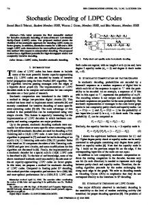
Example 2: In Figures3 3/4 and Figures 5/6 we compare the results for equivalent forms of the PCM we get from Gaussian elimination and from our greedy permutation algorithm. We use the QC-LDPC codes proposed in [6] as realistic example codes, because they are easy to construct and their girth can be analysed [9], which will, in the next section, allow us to find relations between the encoding complexity and the decoding performance (that directly depends on the girth). Both figures clearly indicate the efficiency of the greedy permutation algorithm, as the equivalent SALT forms of the PCMs are still widely sparse (which will allow for efficient encoding) while the Gaussian elimination generates equivalent PCMs with large parts densely populated with “ones”. In our simulations we observed the following properties of the greedy permutation algorithm: 1) Although the greedy permutation algorithm is not globally optimal, the results achieved are always “good” in the sense that the gap is usually small, relative to the 3 In
the figures, a black dot indicates a “one” in the PCM.
IV. S IMULATION R ESULTS
20 40
In Table II we present some simulation results for QCLDPC codes [6]. (The circulant size is a design paramter of the codes; for details see [6]). In the last column of Table II we show the “gap” to linear encoding complexity obtained from our greedy permutation algorithm.
60 80 100 120 140 160
TABLE II
180 50
Fig. 3.
100
150
200
250
300
(305,3,5) LDPC code / Gaussian elimination
20 40 60 80 100 120 140 160 180 50
Fig. 4.
100
150
200
250
300
(305,3,5) LDPC code / Greedy Permutation Algorithm
50
100
150
200
250
300
350
400
GAP OF DIFFERENT CODES FROM GREEDY PERMUTATION ALGORITHM
Block length n 21 93 129 155 186 305 905 905 905 1055 1477 1477 1205 1355 1928 1928 2041 1967 2248 1655 2105 2947 2947
Circulant size m 7 31 43 31 31 61 181 181 181 211 211 211 241 271 241 241 157 281 281 331 421 421 421
Column weight j 2 2 2 3 5 3 3 3 3 3 3 5 3 3 3 5 3 5 5 3 3 3 4
Row weight k 3 3 3 5 6 5 5 5 5 5 7 7 5 5 8 8 13 7 8 5 5 7 7
girth
gap g
12 12 12 8 6 10 8 10 12 12 10 6 12 12 8 8 6 6 6 12 12 10 8
0 0 0 4 34 10 5 17 26 26 12 211 26 20 12 234 3 284 236 41 48 24 173
450
500
100
Fig. 5.
200
300
400
500
600
700
800
900
(905,3,5) LDPC code / Gaussian elimination
50
100
150
200
V.
250
300
350
400
450
500
100
Fig. 6.
We observe that, for a fixed column weight j, a larger girth always means larger gap at the same time. Therefore, there is a fundamental tradeoff between decoding performance (determined by the girth) and low encoding complexity (determined by the gap): a “good” code with high decoding performance will cause higher encoding complexity.
200
300
400
500
600
700
800
900
(905,3,5) LDPC code / Greedy Permutation Algorithm
CONCLUSION
We have investigated the ALT encoding method and presented a new algorithm to transform the original PCM into the ALT form and the SALT form, with small gap to an encoding complexity that grow linearly with the block size. Simulation results demonstrate the efficiency of the new algorithm. VI. ACKNOWLEDGEMENTS
number of rows in the PCM. The results obtained for different choices of rows and colums when there is a tie are always very similar and this applies even if we perform random permutations in the PCM before we start the algorithm. 2) For any regular LDPC code with a column-weight of two (j = 2), the gap is always g = 0, i.e., (2, k) LDPC codes are totally linearly-encodable. 3) Generally, for (j, k) LDPC codes with a column-weight of j > 2 and a row-weight of k > 3, there always exits a lower bound for the minimum gap which is not zero.
This work was supported by Scottish Funding Council for the Joint Research Institute with the Heriot-Watt University which is a part of the Edinburgh Research Partnership. R EFERENCES [1] R. G. Gallager, “Low-density parity-check codes,” IRE Transactions on Information Theory, pp. 21–28, Jan. 1962. [2] T. J. Richardson, M. A. Shokrollahi, and R. L. Urbanke, “Design of capacity-approaching irregular low-density parity check codes,” IEEE Transactions on Information Theory, vol. 47, no. 2, pp. 619–637, Feb. 2001. [3] S. Lin and D. J. Costello, Error Control Coding, Pearson Prentice Hall, 2004.
[4] R. M. Tanner, “A recursive approach to low complexity codes,” IEEE Transactions on Information Theory, vol. 27, no. 5, pp. 533–547, Sept. 1981. [5] M. Luby, M. Mitzenmacher, A. Shokrollahi, D. Spielman, and V. Stemann, “Practical erasure resilient codes,” in Proc. 29th Annu. ACM Symp. Theory of Computing, (STOC), 1997, pp. 150–159. [6] R. M. Tanner, D. Sridhara, A. Sridharan, T. E. Fuja, and D. J. Costello, “LDPC block and convolutional codes based on circulant matrices,” IEEE Transactions on Information Theory, vol. 50, no. 12, pp. 2966–2984, Dec. 2004. [7] C. Di, D. Proietti, I. E. Telatar, T. J. Richardson, and R. L. Urbanke, “Finite-length analysis of low-density parity-check codes on the binary erasure channel,” IEEE Transactions on Information Theory, vol. 48, no. 6, pp. 1570–1579, June 2002. [8] T. J. Richardson R. L. Urbanke, “Efficient encoding of low-density paritycheck codes,” IEEE Transactions on Information Theory, vol. 47, no. 2, pp. 638–656, Feb. 2001. [9] M. P. C. Fossorier, “Quasicyclic low-density parity-check codes from circulant permutation matrices,” IEEE Transactions on Information Theory, vol. 50, no. 8, pp. 1788–1793, Aug. 2004.