WITH MULTIPLE BASE STATIONS AND A CENTRAL CONTROLLER. Martin Fuchs, Giovanni Del Galdo, and Martin Haardt. Ilmenau University of Technology, ...
LOW COMPLEXITY SPATIAL SCHEDULING PROSCHED FOR MIMO SYSTEMS WITH MULTIPLE BASE STATIONS AND A CENTRAL CONTROLLER Martin Fuchs, Giovanni Del Galdo, and Martin Haardt Ilmenau University of Technology, Communications Research Laboratory P.O. Box 10 05 65, 98684 Ilmenau, Germany, Phone +49 (3677) 69 2613 {martin.fuchs, giovanni.delgaldo, martin.haardt}@tu-ilmenau.de ABSTRACT Wireless communications systems with multiple antennas at the transmitter can serve multiple terminals at the same time by exploiting the spatial domain. In a transmission scheme which also uses other orthogonal resources such as time and frequency, a different subset of terminals can be assigned to each resource element. If joint spatial processing is performed at the base station, the subset selection must avoid to group users with spatially correlated channels to prevent a severe throughput degradation. The selection process is computationally very complex because the performance of the spatial processing depends on the user combination to be served. To significantly reduce the complexity, we have developed the ProSched approach. In this contribution we show how it can be extended to schedule terminals in a scenario with multiple interfering base stations and investigate its performance using computer simulations based on the realistic channel model IlmProp. 1. INTRODUCTION We consider the downlink of a MIMO-OFDM mobile communications system in which traffic of adjacent base stations (BS) or access points (AP) is not separated by any means such as orthogonal spreading codes or a fixed bandwidth sharing. The resources time and frequency are assumed to be partitioned in a number of orthogonal resource elements. In each element, a different subset of the U terminals in the system can be served, while each user can also receive multiple spatially separated data streams at the same time. The user selection process for each resource element will be referred to as scheduling. The access points are assumed to be connected via a backbone network and to be able to coordinate their traffic or have it organized by a central controller. Two different coordination strategies will be considered. The first one is often called The authors gratefully acknowledge the partial support of the German Research Foundation (Deutsche Forschungsgemeinschaft, DFG) under contract no. HA 2239/1-1.
distributed MIMO and has recently attracted considerable interest [1]. It implies that all spatial processing is done jointly as if all BS antennas were located at one device and that intracell interference does not exist. In the second strategy, only the scheduling is centrally coordinated while the spatial processing is not. As a result, the interference originating from other base stations has to be considered during the scheduling process. Apart from the interference, the implications of the spatial domain on the terminal scheduling process are the same in both strategies: Terminals with highly spatially correlated channels must not be assigned to the same SDMA group. High spatial correlation severely degrades the possible throughput of any SDMA scheme, because it impairs the spatial separability of the terminals, leading to less efficient precoding matrices and to increased interference. Additionally, the size of a group has a significant impact on the overall performance, because the SDMA throughput gain comes at the expense of serving each user with a smaller fraction of the available transmit power. The ProSched approach [2] considers all of the above issues by using a low complexity estimate of a user’s channel capacity as scheduling metric. It is applicable in the case where channel knowledge is used for SDMA at the transmitter, i.e., no additional channel quality feedback is required. The result of the precoding depends on the user selection, but ProSched reduces the effort of estimating it by using the concept of orthogonal projections to an effort comparable to when a user is served alone. Additionally, the complexity of testing all possible terminal combinations for each SDMA group is avoided with the help of a tree-based search algorithm.
2. SYSTEM MODEL A frame in time is assumed to consist of a number of time slots n. At first, spatial scheduling will be considered without Quality of Service (QoS) requirements. Therefore, it relies solely on the channel state information (CSI), which is assumed to be available once per time frame and consequently, the scheduling solution will be the same for every time slot in a frame. At a time slot n, each orthogonal resource f
in frequency can be used to serve an independently chosen subset of users with size to be determined by the algorithm, where neighbouring OFDM subcarriers can share the same solution, as shown later. This model has advantages over our previous approach, which was pursued in [3] and is used in similar ways in other algorithms, e.g., [4]: there, all terminals are partitioned into a number of groups and one group is assigned to each resource element. The first problem in the old approach is that a multiple of the found number of groups does not necessarily match the number of available resource elements. For example, the algorithm might suggest to form three groups out of the U users in the system. In a system with time frame length ten, groups would have be to repeatedly used to fill up the frame, rendering the system unfair. Furthermore, consider for example U = 5, then a partitioning could be (1, 2)(3, 4)(5) and every third time slot would provide no SDMA gain since it contained only one user. Until mentioned otherwise, the case in which the system has only one BS is considered. For each subcarrier and OFDM symbol, the complex data symbols to be transmitted to user number g ∈ N, 1 ≤ g ≤ G in a group of scheduled terminals G(n, f ) of size G are contained in the column vector dg . The channels on each subcarrier are assumed to be frequency flat. Time and frequency indices will furtheron be skipped for notational simplicity. The complex received data vector for user g is then yg = Hg Mg dg +
G X
Hg Mj dj + ng ,
(1)
j=1,j6=g
where Hg denotes the MR,g × MT complex channel matrix between the MT transmit antennas of the base station and the MR,g receive antennas of user g. Let further Mg denote a linear precoding matrix generated for the transmission to user g. To cover the most general case, the system under consideration shall have the possibility to transmit multiple data streams to each user in an SDMA group. Therefore, Mg is allowed to have up to r = rank {Hg } columns. The elements of vector ng contain the additive noise with power σn2 at each receiving antenna of user g. 3. PROSCHED SCHEDULING METRIC The precoding matrices for all users to be served are generated jointly at the BS. Therefore, the result of the precoding depends on the terminal combination. The first goal of our scheduling approach is to avoid the pre-calculation of the precoding matrices for every user combination of interest during the search for the best user combinations. Instead we use an estimate ηg of the g-th user’s capacity in the group G as scheduling metric for every subcarrier (or resource element in frequency) at every time instant at which the scheduler is executed. Originally, ProSched was derived for a precoding technique called Block Diagonalization (BD) [5], which
forces the interference between the transmissions to the users to be zero. Under this zero-forcing (ZF) constraint, serving users with correlated channel matrices at the same time will lead to a reduction of the channel norm after precoding. ZF implies that user g’s precoding matrix Mg ∈ Cr×r must lie in the joint nullspace of all other users’ channel matrices so that the sum term in equation (1) is zero. In [2] an equivalent formulation of the BD algorithm is given which obtains the same ZF precoding solution as [5]. It is based (0) on an orthogonal projection matrix P˜g which projects Hg ˜ g containing all the chaninto the nullspace of a matrix H nel matrices of all other users in the group except the g-th, � �T T T T ˜ g = H1T ··· Hg−1 Hg+1 ··· HG i.e., H . The (0) MRg ×MT ˚ ˜ resulting matrix Hg Pg = Hg ∈ C fulfils the ZF condition and can in a second step be used together with other MIMO precoding techniques such as SVD based precoding to decompose it into orthogonal spatial modes. In the following, the superscript (0) is added to basis of a null space or a projection into a nullspace and (1) is added to a row space or a projection into a row space. The scheduling metric is defined in [2] as �
2 � PT
(0) ˜ . (2) ηg = log2 1 +
Hg Pg Grg σn2 F As already mentioned, it is an estimate of the link rate for user g and represents a lower bound on the ZF capacity obtained by the BD algorithm. This metric involves the assumption that equal fractions of the available transmit power PT are assigned to the G users in the group and again to all rg spatial modes of a user. This is necessary because the calculation of the full precoding matrix is avoided for the scheduling and thus the optimum power allocation is unknown. Simulations show that this simplification is sufficient for the scheduling process. A way to consider the near-far-effect in large scale scenarios is inherent to the proportional fairness extension addressed in Section 5.1. The main advantage of using this metric is that the projection can be approximated by repeatedly applying projections into the separate users’ nullspaces instead [6]:
� �p (0) (0) (0) (0) , p → ∞. P˜g(0) = P1 · . . . · Pg−1 Pg+1 · . . . · PG (3) These separate projectors can be conveniently computed from (1) a basis Vu for the row space of a user u’s channel matrix as (0) (1) (1)H Pu = I − Vu Vu , where the basis can be obtained via an SVD of Hu . As a result, our algorithm does not re˜ g for every user combination to be quire decompositions of H tested. Instead it requires only U small SVDs at the beginning to obtain the bases of all U users’ row spaces to calcu(0) (0) late the re-usable projectors Pu . A projector P˜g for any user combination is then obtained by simply multiplying the (0) respective projectors Pu . In [2] the approach is therefore
termed ProSched. The number of multiplications needed during the scheduling process is negligible, because p = 1 is already sufficiently accurate to achieve a good grouping of the users and also because rank one approximations of the Vu can be used. In the case where the precoding allows interference (nonZF case), spatially correlated channels also lead to a reduced channel norm and additionally to an increase in interference. The amount of interference produced is related to the channel quality reduction in the ZF case and, therefore, we use the same metric for scheduling, as also discussed in more detail in [2]. For example, the MMSE(TxWF) precoding technique (see, e.g., [7]) used in Section 6 converges to the pseudo inverse of the channel at high SNRs and includes, therefore, the ZF solution as a special case. If the system has B BSs, we distinguish them by an additional subscript b ∈ N, 1 ≤ b ≤ B. Furthermore, let u ∈ N, 1 ≤ u ≤ U , be a “global” user number, whereas g was used above as a ’local’ user number in a group G of size G. The channel between user u and BS b is denoted Hu,b . If the distributed MIMO approach is taken, all BSs are combined to form one virtual BS having a channel matrix H consisting hof all BS’s channel matrices stacked together such that � �T � �T i T T T T ··· HU,1 H1,1 ··· HU,B H = ··· H1,B . The rows of H corresponding to user g-th antennas can then be used in the calculation of the metric in equation (2) as if only one BS was present in the system. If only the scheduling is performed jointly among the BSs but not the spatial processing, any BS sends interference to the users which are not assigned to it and are served by other BSs (intra-cell interference). To estimate the intra-cell interference, we work again with the assumption of a ZF algorithm like BD at the transmitter. The precoding matrix Mg for user number g in a group of size G can be split into a matrix with normalized columns Ng and a diagonal power loading matrix Dg such that Mg = Ng Dg . The diagonal elements of Dg contain the square roots of the fractions of the total transmit power assigned to each spatial mode. The new formulation for BD precoding derived in [2] is used in the fol˚g(1) where V ˚g(1) is a basis of the lowing. Therefore, Ng = V ˚g , obtainable, e.g., via row space of the projected channel H ˚g . SVD. It represents the spatial modes of H To calculate the interference estimate for one user of interest u, let the BS serving it be assigned number b = 1. To simplify the notation, we consider only the hard handover scenario. Let there be another BS b > 1 which is not serving u. Its transmition to a user with local user number 1 ≤ g ≤ Gb out of its assigned group Gb creates interference for user u with the following receive covariance matrix H
˚ (1) Dg D H V ˚ (1) H H , Ru,b,g = Hu,b V g g g u,b
(4)
under the usual assumption�of uncorrelated data symbols with average unit power, i.e., E dg dH = I. Since our algorithm g
works with low complexity estimates and avoids the calcula˚g(1) is not known tion of the full precoding matrix, the basis V to the scheduler. Using the p above mentioned equal power loading assumption Dg = PT /(G · rg )I, Ru,b becomes Ru,b,g
=
=
PT ˚ (1) V ˚ (1)H H H Hu,b V g g u,b G · rg PT ˚(1) P ˚(1) H H . Hu,b P g g u,b G · rg
(5)
H
˚g(1) V ˚g(1) = P ˚g(1) is an othogonal projection maThe term V trix into the row space of user g’s zero forced channel. Projectors are idempotent, therefore it can be multiplied a second time. Generally, the interference is highly directional due to the spatial processing and differs at each receive antenna of a user. However, our scheduling metric uses a scalar norm of the projected channel and, therefore, only a scalar interference power term can be considered as an increment of the noise power term σn2 . It was confirmed during simulations that scheduling does not demand a highly accurate intra-cell interference 2 estimate. Let us define σi,u,b,g = trace {Ru,b,g } which represents the total estimated intercell-interference power received by user u generated by BS b while serving user g out of its assigned group, then the following holds: � � PT 2 ˚(1) P ˚(1) H H σi,u,b,g = trace Hu,b P g g u,b G · rg
2 PT ˚(1) (6) =
Hu,b P g . G · rg F The Frobenius norm term expresses the similarity between the subspace into which the BS transmits and the subspace of the user receiving interference. We can exploit the fact that the row space of a matrix is an orthogonal complement of its null space: �
2 �
PT
2 (0) 2 ˚ , (7) kHu,b kF − Hu,b Pg σi,u,b,g = G · rg F
which is the equivalent of Pythagoras’ theorem for multi(0) dimensional subspaces. Let V˜g represent the nullspace ˜ g containing all the channel matrices of all of the matrix H ˚g(1) projects other users in the group except the g-th. Since P (0) into a subspace contained by V˜g , we can replace Hu,b by (0) Hu,b P˜g such that �
2
2 � PT
2 (0) (0) ˚(0) ˜ ˜ σi,u,b,g = .
Hu,b Pg − Hu,b Pg Pg G · rg F F (8) (0) ˚(0) ˜ The projection matrix obtained by the product Pg Pg is equal to the projector into the subspace obtained by the in(0) (0) tersection between V˜g and Vg . Therefore, exploiting the same approximation shown in equation (3), we can write � �p ˚(0) = P˜ (0) P (1) P˜g(0) P , p → ∞. (9) g g g
This approximation allows us to write the total estimated intercell-interference power as �
2 �p 2 � � PT
(0) (0) 2 (0) ˜ ˜ σi,u,b,g =
.
Hu,b Pg − Hu,b Pg Pg G·rg F F (10) (0) ˜ This notation is particularly convenient because both Pg (0) and Pg need to be computed anyhow for the scheduling metric so that no additional SVDs are required. Again the number of repeated projections p determines the accuracy. In the simulations it is set to the same value as for the approxi(0) mation of P˜g . Consequently, the total intra-cell interference power received by user u is the sum of all intra-cell interference generated by all other BSs while serving their assigned users: 2 σi,u =
B X X
2 σi,u,b,k .
(11)
45 123 4 123 4 12
11 22
11
22
55
33
55
33
44
55
33
44
55
User numbers
Fig. 1. An example for the sorting tree used in the scheduler at one time instance: in a system with 5 users, candidate user sets of sizes 1 to 5 are produced with the help of a best candidate combining procedure and a scheduling metric reflecting the performance of the groups. In the final step the algorithm selects among the candidate sets appearing on the left.
b=2 k∈Gb
The scheduling metric for user g in a group Gb with intra-cell interference then becomes !
2
PT
˜ (0) . (12) ηg = log2 1 + 2 ) Hg Pg Grg (σn2 + σi,g F 4. TREE-BASED SORTING ALGORITHM
To reduce the number of terminal combinations to be tested for maximum throughput, a best candidate search algorithm in the form of a dendrogram (or search tree) is used. It can work with our metric or any other kind of metric which represents an estimate of a user’s link quality. The algorithm consists of two phases. In the first phase, candidate user groups in all possible sizes from one to the maximum size supported by the precoder are identified (typically the rank of the combined downlink channel matrix). To do so, in the case of only one (virtual) BS, the first phase starts with single user groups containing terminals 1 . . . U which form the first level of the tree as shown in Figure 1 for U = 5 users. The terminal with the best metric is identified and is assigned number one. Next, the pairing with the highest metric sum of user one with any of the remaining users is searched for and stored as candidate grouping with size two. In the example, this candidate grouping contains users one and two. The algorithm continues in this way until candidate groups for all possible sizes have been found. They appear on the left edge of the tree as marked in gray. In the second phase, the group with the highest metric sum out of the candidate groups is selected as the scheduling solution for the current time slot and frequency resource. The final selection can also be performed by calculating the true rates for the few candidate sets. This eliminates the estimation error in this step of the algorithm and can increase its performance. Please note that a pseudo code algorithm description is given in [2].
The algorithm can be extended to the case of multiple BSs which only perform scheduling jointly. To do so, the scheduling metric must contain the influence of the interference. The tree is started with U · B ’virtual’ users representing all possible combinations of users and BSs. By applying the tree as it is on those virtual users, a soft handover-like strategy is obtained, i.e., more than one BS can be allowed to serve a terminal. To achieve a hard handover, once a physical terminal has been assigned to a candidate grouping solution, all of its other virtual representations must be deleted from the current tree level before the next level is calculated. In the soft handover case, the calculation of the rate estimate must take into account the receiver strategy. In our case it is assumed that all spatial modes are used by a BS to transmit to a user. Therefore, all BSs serving a single user are assumed to share a time slot via an additional TDMA or CDMA scheme and the metric for each link is divided by the number of BSs serving a user. Alternatively, each BS could for example only use the dominant spatial mode, allowing the user to employ a VBLAST like receiver on the stacked channel matrix H to detect multiple serving BSs at the same time. It is also to be decided whether diversity or SDMA gain should be the goal of a soft handover, but this is beyond the scope of this investigation. 5. ALGORITHM EXTENSIONS 5.1. Fairness, QoS, and long term CSI Our scheduling metric is a rate estimate. Therefore, it can be combined with other existing approaches for QoS and fairness which are based on the calculation of user rates. In [2], examples are given how proportional fairness [8] in the form of methods given in [9] can be implemented and user rate requirements or user service priorities can be considered as
in [10] or [11]. Also in [2] a method for scheduling on long term channel knowledge was investigated. If the channel varies too rapidly to be tracked by the estimation algorithm in use, [12] uses averaged spatial covariance matrices of each user’s channel matrix instead to obtain the basis of the row space for the multi-user precoding. This principle is also applicable for scheduling (see also next section). 5.2. Complexity reduction in frequency and time It is known that a wireless channel transfer function displays correlation between the bins in the discrete frequency domain. The complexity of spatial processing can, therefore, be reduced by performing it only once for a cluster of correlated frequency bins and then replicating the solution on all C bins within the cluster at the expense of accuracy. The method mentioned above for precoding/scheduling on long term CSI [12] was modified in [13] for usage with multi-user precoding in the frequency domain. Here we investigate how our scheduling algorithm performs with it: within a cluster number c, the scheduling is performed only once with a pseudo ˆ u,b (c) for each user u instead of using the channel matrix H measured channel matrix Hu,b (f ) on every subcarrier. In the distributed MIMO case, the same principle can be applied to the respective rows of H. To do so, first an estimated transmit covariance matrix RT,u,b (c) is calculated for each cluster c using averaging: RT,u,b (c) =
C 1 X H Hu,b (f )Hu,b (f ) . C
(13)
f =1
ˆ u,b is constructed from a basis The pseudo channel matrix H of the signal space of RT,u,b (c) which can for example be obtained with an EVD RT,u,b (c)
such that (1)
H = Uu,b Σu,b Uu,b h (1) = Uu,b Σu,b Uu,b
(0)
Uu,b H
ˆ u,b (c) = Σ1/2 U (1) , H u,b u,b
iH
(14)
where Uu,b contains the first r = rank {Hu,b (c)} columns of Uu,b . Two more complexity reduction methods are given in [2]. It is possible to track the solution found by the tree based algorithm in time. Instead of building the entire tree at every instance of the scheduler, only a number of levels above and below the previously found solution are calculated. This is possible with the help of an equivalent tree algorithm which proceeds top-down. In our simulations we calculate only one level above the previous solution and then proceed down two levels to update also the past solution. This tracking is especially attractive when all users on all subcarriers are treated in one big tree. To do so, all users’ channels from all subcarriers
Fig. 2. The IlmProp scenario used for simulations: up to U = 24 mobile stations (red) move randomly in an area with two base stations. (or clusters) are considered as one frequency flat system and the tree is started with U · N · B virtual users (N being the number of subcarriers or clusters). The calculation of the metrics has to take into account the orthogonality of virtual users originating from different subcarriers. In our simulations we still update only three levels when using this virtual system together with the tracking in time. 6. SIMULATIONS For our simulations, a two-BS MIMO scenario with up to U = 24 users moving randomly at speeds of up to 70 km/h is used as shown in Figure 2. It is generated with the geometry based channel model IlmProp [14] featuring realistic correlation in space, time, and frequency between users. This is crucial in assessing the performance of a spatial scheduling scheme. The BSs have 12 element uniform circular arrays while each user has two onmidirectional antennas, λ/2 spaced. To illustrate the effectiveness of different variations of our algorithm, Figure 3 shows a comparison with the performance of user selections found by exhaustively searching through all possible user subsets as well as to a trivial Round Robin scheduler with different maximum group sizes as explained below. Due to the computational complexity of an exhaustive search this is only shown in the scenario when the two BS schedule jointly but precode separately and only for the frequency flat case at a frequency of 2 GHz, for a single SNR value and a total of 10 users. SNR is defined as total transmit power over receiver noise variance. Consequently, the results are given as complementary cumulative distribution functions of the total system rate. Since the basic algorithm itself is not affected by the physical parameters, we calculate only normalized performance estimates to show the relative gains between the algorithms. An OFDM symbol duration of 20 µs is assumed without considering the length of the guard period and a TDMA frame consisting of 50 OFDM symbols. We show the case in which the two BSs perform only the scheduling jointly and do BD precoding and water pouring separately. Ideal power loading is used to calculate the resulting rates
Comparison of scheduling methods for BD precoding and 2 BSs 1 Complementary CDF on one subcarrier
(but not within the scheduling metric), assuming that in a real world implementation a power and bit loading algorithm with the goal of increasing throughput such as in [15] can be used. Our algorithm reaches a performance close to the exhaustive search in all displayed variations. The following abbreviations are used in the legend: ProSched.full.p=1 stands for our projection based algorithm using full basis matrices and an order of p = 1 for the repeated projection approximations. ProSched.rank1.p=1 indicates that reduced rank basis matrices are used in the calculation of the projection matrices. In the tree based algorithm, the final solution can be selected with the help of the scheduling metric (pick=metric) or based on the true rate (pick=rate). The suffix tracking stands for the complexity reduction method in time by tracking of the search tree. The first conclusion is that an essentially random scheduler like Round Robin is not recommended. The risk of scheduling a user with blocked propagation paths to any BS even increases when bigger groups are chosen and, therefore, even TDMA performs better in our simulations than SDMA. The next conclusion is that the second step of the tree based algorithm, i.e., the selection among the candidate user subsets, is especially sensitive to the estimation error in our metric. Therefore, it is recommended to use the calculated rate for this step and on the other hand reduce the complexity again with the help of the time tracking algorithm (which reduces the number of candidate sets to choose from to three only). In Figure 4, simulation results for the frequency selective case with 24 frequency bins spanning a bandwidth of 1.2 MHz and 24 users are shown in the form of 90% outage curves as a function of SNR. The scheduling algorithm in use is the one which displayed the best trade-off in complexity and performance in the frequency flat case, namely ProSched.rank1.p=1.pick=rate.tracking. This time MMSE(TxWF) precoding [7] is used. We emphasize the comparison between the distributed MIMO approach with one virtual BS and the case with separate spatial processing (where the receiver strategy is dicussed in Section 4). We observe that Round Robin performs surprisingly well in the virtual MIMO case for low SNRs. The more important conclusion is that two separate BSs outperform the virtual MIMO approach. This is due to the fact that in this scenario with relatively short distances users are very often assigned to two BSs at the same time. And although the two BSs have to share the time slot in our system model, it is more beneficial for the users to be served by two times two spatial modes rather than by only two modes with slightly higher quality in the virtual MIMO case. For the two BS case, a curve was simulated with the frequency averaging method from Section 5.2 where the bandwidth was divided into four clusters of six bins. In the legend it is marked with the suffix clustering. The performance difference due to the reduced accuracy is negligible. Note that the averaging was used only for the scheduling and not for the precoding to assess its implications on the scheduler only.
0.8
0.6
0.4
0.2
0
0.5 1 1.5 2 2.5 Total system throughput [bps/Hz] at fixed SNR SDMA MAX. exhaustive search SDMA RoundRobin−12 SDMA RoundRobin−8 TDMA=RoundRobin−2 ProSched.full.p=3.pick=rate ProSched.full.p=3.pick=metric ProSched.rank1.p=1.pick=rate ProSched.rank1.p=1.pick=rate.tracking ProSched.rank1.p=1.pick=metric ProSched.rank1.p=1.pick=metric.tracking
Fig. 3. Variations of ProSched with different complexity compared to an exhaustive search over all possible combinations in the given scenario with two BSs and 10 mobile stations. The curve belonging to the method which offers the best performance vs. complexity trade-off is marked with an ’o’. Definition of the Round Robin scheme: The Round Robin scheme re-schedules every time slot. For the frequency selective case, the same solution is applied to all subcarriers. In the legends, the number after Round Robin denotes how many users are to be scheduled at every time slot. In the distributed MIMO case the 24 element array at the virtual base station can spatially multiplex up to 12 users, with two antennas each. The RR-X scheme selects X users, by cycling through the U available. For instance, a RoundRobin5 scheme would schedule the following users out of U = 12 for successive time snapshots: {1, 2, 3, 4, 5}, {6, 7, 8, 9, 10}, {11, 12, 1, 2, 3}, etc. In the case of two separate BSs, each BS can serve at most six users. To obtain the Round Robin solution, we split the one BS case into two parts, effectively cycling the user assignment also through the two BSs.
7. CONCLUSION In the downlink of MIMO systems with SDMA, scheduling is required to prevent the huge performance losses due to spatially correlated users and to fully exploit the gains offered
Total system rate at 90% outage (normalized)
Frequency selective case with MMSE(TxWF) precoding 10 9
[1] M. Dohler, A. Gkelias, and H. Aghvami, “A resource allocation strategy for distributed MIMO multi-hop communication systems,” IEEE Communications Letters, vol. 8, no. 2, pp. 99 – 101, February 2004.
8 7 6
[2] M. Fuchs, G. Del Galdo, and M. Haardt, “Low complexity space-time-frequency scheduling for MIMO systems with SDMA,” submitted for publication.
5 4 3 2 1 0 −15
8. REFERENCES
−10
−5
0 5 10 15 20 SNR/dB 2 BSs joint scheduling: ProSched.rank1.p=1.pick=rate.tracking ProSched.rank1.p=1.pick=rate.tracking.clustering virtual MIMO: ProSched.rank1.p=1.pick=rate.tracking SDMA RoundRobin−12 TDMA=RoundRobin−1
Fig. 4. Comparison of the virtual MIMO approach with two separate BSs performing joint scheduling in the frequency selective case with 24 mobile stations and MMSE(TxWF) precoding.
[3] ——, “A novel tree-based scheduling algorithm for the downlink of multi-user MIMO systems with ZF beamforming,” in Proc. IEEE Int. Conf. Acoust., Speech, Signal Processing (ICASSP), vol. 3, Philadelphia, PA, March 2005, pp. 1121–1124. [4] F. M. Wilson and A. W. Jeffries, “Adaptive SDMA downlink beamforming for broadband wireless networks,” in Proc. Wireless World Research Forum Meeting 14, San Diego, CA, July 2005. [5] Q. H. Spencer, A. L. Swindlehurst, and M. Haardt, “Zero-forcing methods for downlink spatial multiplexing in Multiuser MIMO channels,” IEEE Transactions on Signal Processing, vol. 52, no. 2, pp. 461–471, February 2004. [6] I. Halperin, “The product of projection operators,” Acta. Sci. Math. (Szeged), vol. 23, pp. 96–99, 1962.
by multi-user diversity in SDMA. Our algorithm ProSched, which is based on a way of interpreting the process of precoding with the help of orthogonal projectors, on an efficient search algorithm, and on approximation techniques, can reach a performance close to the one obtained by exhaustively searching through all user combinations.PFor one �BS with U = 10 R U = 1023 comusers, the latter requires to test G=1 G binations on every subcarrier. In the case of BD precoding, two SVDs are required per combination yielding 2046 SVDs. As derived in [2], using the tree based search without the time tracking modification tests 340 combinations but requires only 10 SVDs in total. The ProSched algorithm can treat space, time, and frequency jointly. It not only considers the spatial correlation but inherently also the degree of freedom in choosing the right SDMA group size. Our approach is not restricted to a specific type of spatial precoder and can be applied to systems with long-term channel knowledge based on second order statistics only. It is possible to include proportional fairness and QoS into the algorithm. Here, the algorithm is extended to either schedule users jointly for multiple base stations or to be applied in a distributed MIMO scheme. In our simulations it was observed that joint scheduling outperforms the virtual MIMO approach.
[7] M. Joham, J. Brehmer, and W. Utschick, “MMSE approaches to multiuser spatio-temporal TomlinsonHarashima precoding,” in Proc. 5th International ITG Conference on Source and Channel Coding (ITG SCC’04), January 2004, pp. 387–394. [8] J. Holtzman, “Asymptotic analysis of proportional fair algorithm,” in 12th IEEE International Symposium on Personal, Indoor and Mobile Radio Communications (PIMRC), vol. 2, 2001, pp. 33–37. [9] T. Bonald, “A score-based opportunistic scheduler for fading radio channels,” in The Fifth European Wireless Conference EW, Barcelona, Spain, February 2004. [10] M. Schacht, “System performance gains from smart antenna concepts in CDMA,” Ph.D. dissertation, University Duisburg-Essen, Germany, February 2005, appearing in: Selected Topics on Communications, Shaker Verlag. [11] P. Svedman, S. K. Wilson, and B. Ottersten, “A QoS-aware proportional fair scheduler for opportunistic OFDM,” in IEEE 60th Vehicular Technology Conference, 2004. VTC2004-Fall, vol. 1, 2004, pp. 558 – 562.
[12] V. Stankovic and M. Haardt, “Multi-user MIMO downlink beamforming over correlated MIMO channels,” in Proc. International ITG/IEEE Workshop on Smart Antennas (WSA05), Duisburg, Germany, April 2005. [13] “IST-2003-507581 WINNER: D2.10 final report on identified RI key technologies, system concept, and their assessment; Appendix G.2.5 Performance of SMMSE precoding,” December 2005. [14] More information on the model, as well as the source code and some exemplary scenarios can be found at http://tu-ilmenau.de/ilmprop. [15] D. Bartolome and A. I. Perez-Neira, “Multiuser spatial scheduling in the downlink of wireless systems,” in Proc. IEEE SAM04 Conference, Spain, July 2004.