Hindawi Publishing Corporation Journal of Sensors Volume 2013, Article ID 197090, 10 pages http://dx.doi.org/10.1155/2013/197090
Research Article Low-Cost MEMS-Based Pedestrian Navigation Technique for GPS-Denied Areas Abdelrahman Ali and Naser El-Sheimy Department of Geomatics Engineering, The University of Calgary, 2500 University Drive N.W., Calgary, AB, Canada T2N 1N4 Correspondence should be addressed to Abdelrahman Ali;
[email protected] Received 10 April 2013; Accepted 22 July 2013 Academic Editor: Kai-Wei Chiang Copyright © 2013 A. Ali and N. El-Sheimy. This is an open access article distributed under the Creative Commons Attribution License, which permits unrestricted use, distribution, and reproduction in any medium, provided the original work is properly cited. The progress in the micro electro mechanical system (MEMS) sensors technology in size, cost, weight, and power consumption allows for new research opportunities in the navigation field. Today, most of smartphones, tablets, and other handheld devices are fully packed with the required sensors for any navigation system such as GPS, gyroscope, accelerometer, magnetometer, and pressure sensors. For seamless navigation, the sensors’ signal quality and the sensors availability are major challenges. Heading estimation is a fundamental challenge in the GPS-denied environments; therefore, targeting accurate attitude estimation is considered significant contribution to the overall navigation error. For that end, this research targets an improved pedestrian navigation by developing sensors fusion technique to exploit the gyroscope, magnetometer, and accelerometer data for device attitude estimation in the different environments based on quaternion mechanization. Results indicate that the improvement in the traveled distance and the heading estimations is capable of reducing the overall position error to be less than 15 m in the harsh environments.
1. Introduction Personal navigation requires technologies that are immune to signal obstructions and fading. One of the major challenges is obtaining a good heading solution in different environments and for different user positions without external absolute reference signals. Part of this challenge arises from the complexity and freedom of movement of a typical handheld user where the heading observability considerably degrades in low-speed walking, making this problem even more challenging. However, for short periods, the relative attitude and heading information is quite reliable. Self-contained systems requiring minimal infrastructure, for example, inertial measurement units (IMUs), stand as a viable option, since pedestrian navigation is not only focused on outdoor navigation but also on indoor navigation. Nowadays, most of the smartphones are programmable and equipped with self-contained, low cost, small size, and power-efficient sensors, such as magnetometers, gyroscopes, and accelerometers. Hence, integrating IMUs navigation
solution with a magnetometer-based heading can play an important role in pedestrian navigation in all environments. In the current state of the art in MEMS technology, the accuracy of gyroscopes is not good enough for deriving an absolute heading or relative heading over longer durations of time. However, for short periods, the relative attitude information is quite reliable. Magnetometers, on the other hand, provide absolute heading information once calibrated. However, they can easily be disturbed by ferrous objects nearby, making them unreliable for brief intervals. This calls for the investigation of possible sources of heading error in complementary sensors such as a gyroscope and a magnetometer and improving the accuracy of the result based on an improved Kalman filter design. Much research towards the heading estimation for personal positioning applications has been conducted in the recent years. Some approaches use magnetometers exclusively for heading estimation [1] while others integrate it tightly with an IMU [2, 3]. One commercially available personal locator system based on this principle is
2 the Dead Reckoning Module DRM-4000 made by Honeywell [4]. A quaternion-based method to integrate IMU with magnetometer is presented by [5]. Three body angular rates and four quaternion elements were used to express attitude and were selected as the states of the Kalman filter. The method needs to model the angular motion of the body. In [6], a linear system error model based on the Euler angles errors expressing the local frame errors is developed, and the corresponding system observation model is derived. The proposed method does not need to model the system angular motion and also avoids the nonlinear problem which is inherent in the customarily used methods. A similar technique is proposed by [7] where the angular rates were modeled to be a constant. A nonlinear derivative equation for the Euler angle integration kinematics is investigated in [8]. Work in [9, 10] presented an Euler angle error based method to integrate IMU with magnetometer data where three Euler angle errors and three gyroscope biases were used as states for the Kalman filter. The estimated states were used to correct the Euler angles and to compensate gyroscope drifts, respectively. The work at [11] presented a mathematical model for compass deviation by creating an a priori look-up table for heading corrections. A Kalman filtering approach was investigated by [12] to estimate the angular rotation from the input of a magnetometer compass and three gyroscopes. References [13, 14] presented a least squares technique with improvement which is used for the estimation of the compass deviation model. In addition, much research has been conducted to use the 3D magnetometer-based heading for personal navigation applications in the recent years [15]. The magnetometer cannot be used as standalone source for heading information in the harsh environments, especially indoor [16]. In addition, it is required to have knowledge about the preexisted magnetic anomalies resulted from some of the man-made infrastructure [17]. Using magnetic field measurements in heading estimation for indoor navigation also has some limitations as the magnetic field signal needs to be strong enough. Also, the mobile navigation device should be away from any source of disturbances to avoid any perturbation effect [18]. Besides that, the magnetic field during the indoor environment is not completely constant due to the presence of the electronic and electrical devices everywhere. To avoid the problem of magnetometer anomaly, arising out of ferrous materials in the vicinity of the magnetometers, a perturbation detection technique is required. In such scenario, the filter works only in the propagation mode without any update for the attitude. Also the gyroscope bias drifts with time and temperature can be compensated by magnetometers. In this paper, a method is presented to obtain seamless attitude information by integrating the heading outputs based on magnetometer, accelerometer, and gyroscope measurements using the Kalman filter (KF).
2. Pedestrian Dead Reckoning (PDR) Pedestrian dead reckoning is a relative means of positioning where the initial position and heading of the user are supposed to be known. The basic concept and components of the
Journal of Sensors Table 1: Sensors manufacture and ranges. Sensor Gyroscope Accelerometer Magnetometer
Manufacture mpu-3050 BMA220 YAS530
Range ±250 to ±2000∘ /sec ±2, ±4, ±8, ±16 g ±800 𝜇T
proposed PDR algorithm are shown in Figure 1. Generally, steps of the user are detected based on the accelerometer data. To get the travelled distance, the total number of steps is multiplied by the step length. With known heading and reference point, the user can be tracked by successive steps count. Step detection is a basic step for any PDR algorithm. Usually, the accelerometer signal is used to detect the steps of the person. Once the step is detected, the total number of steps for a pedestrian can be counted. As a result, the total travelled distance can be estimated by multiplying the step length with the total number of steps. Using travelled distance and heading, user can be located during a typical trip. Step detection algorithm can be performed based on different kinds of sensors, that is, not only accelerometers but even gyroscopes and magnetometers. However, our step event detection scheme is based on using the accelerometer signal. The norm of the three accelerometers is used as in (1), where it is possible to clearly identify the steps by observing, for example, the signal over time: accelnorm = √(𝐹𝑥2 + 𝐹𝑦2 + 𝐹𝑧2 ).
(1)
Steps are detected as peaks in the resulting norm, where the step is the highest local maximum in the norm acceleration between the current peak and the previous step peak.
3. Sensors Performance The used device in the test, Samsung Galaxy Nexus smartphone, is shown in Figure 2 with axes definition. Besides other sensors, the device is equipped with triad magnetometer (M), triad gyroscope (G), and triad accelerometer (A). The manufactures and the ranges of the main used sensors are listed in Table 1. 3.1. Gyroscope Drift. Gyroscopes are mainly used to determine device attitude. The output of such sensor is rotational rate, and performing a single integration on the gyroscopes outputs is necessary to obtain a relative change in angle. Due to the integration process which is very sensible to the systematic errors of the gyroscopes, the bias introduces a quadratic error in the velocity and a cubic error in the position [19]. Gyroscopes measurements can generally be described using 𝐼𝜔 = 𝜔 + 𝑏𝜔 + 𝑆𝜔 + 𝑁𝜔 + 𝜀 (𝜔) ,
(2)
where 𝐼𝜔 is the measured angular rate, 𝜔 is the true angular rate, 𝑏𝜔 is the gyroscope bias, 𝑆 is the linear scale factor matrix, 𝑁 is the nonorthogonality matrix, and 𝜀(𝜔) is the sensor
Journal of Sensors
3 3D gyroscope
3D magnetometer
Measurements leveling
Measurements leveling
Initial orientation
3D accelerometer
Measurements leveling
Multi-heading fusion technique (device heading)
Misalignment estimation
User heading estimation
Initial position and attitude
PDR algorithm
Step detection/ length estimation
Navigate the user
Figure 1: The main concept of the PDR algorithm.
Y (lateral)
X (forward)
Z vertical (down)
Figure 2: Device axis definition.
noise. With integration, the gyroscope bias will introduce an angle error in pitch or roll proportional to time; that is, 𝛿𝜃 = ∫ 𝑏𝜔 𝑑𝑡 = 𝑏𝜔 𝑡; this small angle will cause misalignment of the IMU. Therefore, when projecting the acceleration from for example the gravity vector 𝑔, from the body frame to the local-level frame, the acceleration vector will be incorrectly projected due to this misalignment error. This will introduce an error in one of the horizontal acceleration; that is, 𝛿𝑎 = 𝑔 sin(𝛿𝜃) ≈ 𝑔𝛿𝜃 ≈ 𝑔𝑏𝜔 𝑡. Consequently, this leads to an error in velocity 𝛿V = ∫ 𝑏𝜔 𝑔𝑡 𝑑𝑡 = (1/2) 𝑏𝜔 𝑔𝑡2 and in position 𝛿𝑝 = ∫ 𝛿V 𝑑𝑡 = ∫(1/2)𝑏𝜔 𝑔𝑡2 𝑑𝑡 = (1/6)𝑏𝜔 𝑔𝑡3 . To overcome the problem of error drift, a bias compensation of gyroscopes is required. When the device is in stationary mode, the deterministic bias of the gyroscope can be estimated by calculating the average gyroscope output during that time.
3.2. Magnetometer Perturbation. During operation, especially inside buildings, a magnetometer is subject to many external disturbances such as large metal objects [20]. Other objects like steel structures and electromagnetic power lines can affect the solution of the magnetometer. These kinds of disturbance lead to unpredictable performance of the magnetometer which is a major drawback of using magnetic sensors. In the meanwhile, the magnetic field parameters such as strength, horizontal and vertical magnetic field, and change in the inclination angle can be checked to detect the perturbation in magnetometer measurement by comparing to the reference values which can be found at [21]. Figure 3 shows an example for harsh environment as the magnetometer is totally disturbed due to the steel constructions. The figure shows the total magnetic field in a perturbed area during a walking test compared to the reference value which is 570 mGauss for Calgary [21].
4. Multisensors Heading Fusion Filter The attitude of the device is commonly estimated using the inertial sensor. There are three main approaches for attitude representation: DCM, Euler angle, and quaternion. Among the three techniques quaternion algebra is the preferred. However, the estimated attitude from the gyroscope is very noisy leading to unbounded growth in the heading errors. An integration scheme for the gyroscope, accelerometer, and magnetometer data is proposed to estimate the device attitude and the gyroscope bias. The proposed scheme is a quaternion-based KF as shown in Figure 4. In order to use the KF-based estimator for quaternion parameters and gyroscope biases estimation for a device which is carried by a pedestrian, the required model for the states and measurements and their respective system and measurement error models are presented in this section.
4
Journal of Sensors The matrix transforms from the body frame to the local level (navigation) frame. The roll, pitch, and azimuth values can be obtained by using the 𝑎 tan 2 math function on the values of the 𝐶𝑛 propagated inside the sensors navigation equations 𝜙 = tan−1 ( Steel
𝜃 = −sin−1 (𝐶𝑛 (1, 3)) ,
(a) The structure at the CCIT 2nd floor
Magnetic field (mGauss)
𝜓 = tan−1 (
Total magnetic field
900
(6)
𝐶𝑛 (1, 2) ). 𝐶𝑛 (1, 1)
4.2. Filter States. Basically, the target of the proposed filter is to estimate the device attitude based on the quaternion technique. Consequently, any improvement in the quaternion estimate leads to improving the estimated attitude values. The implementation of the KF is optimal for linear systems driven by additive white Gaussian noise (AWGN). The state model can be written in the following form:
800 700 600 500 400 300
𝐶𝑛 (2, 3) ), 𝐶𝑛 (3, 3)
𝑥̇ = 𝐹𝑥 + 𝐺𝑤, 0
100
200
300 Time (s)
400
500
600
Normal area Perturbed area Reference value
where 𝑥 is the state vector, 𝐹 is the state transition matrix, and 𝐺𝑤 represents the covariance matrix of the applied state model. The measurement system can be represented by a linear equation of the following form: 𝑍 = 𝐻𝑥 + V,
(b) Total magnetic field
Figure 3: Magnetic field perturbation.
4.1. Quaternion Mechanization. The relationship between the direct cosine matrix (DCM) and Euler angles is given in (3) with the sequence of azimuth, pitch, and roll (𝜓𝜃𝜙) or 𝑦 (𝑅𝜙𝑥 𝑅𝜃 𝑅𝜓𝑧 ) [22]: 𝐶𝑙𝑏
𝑐𝜃𝑐𝜓 𝑐𝜃𝑠𝜓 −𝑠𝜃 [𝑠𝜙𝑠𝜃𝑐𝜓 − 𝑐𝜙𝑠𝜓 𝑠𝜙𝑠𝜃𝑠𝜓 + 𝑐𝜙𝑐𝜓 𝑠𝜙𝑐𝜃] =[ ].
(3)
[𝑐𝜙𝑠𝜃𝑐𝜓 + 𝑠𝜙𝑠𝜓 𝑐𝜙𝑠𝜃𝑠𝜓 − 𝑠𝜙𝑐𝜓 𝑐𝜙𝑐𝜃] A quaternion is a four-dimensional vector which is defined based on a vector 𝑞 and a rotation angle. The vector 𝑞 is given as 𝑞 = (𝑞1 , 𝑞2 , 𝑞3 , 𝑞4 ) .
(4)
The DCM matrix in terms of quaternion vector components can be obtained from using 2𝑞12
𝑞22
−1+ 2𝑞2 𝑞3 + 2𝑞1 𝑞4 2𝑞2 𝑞4 − 2𝑞1 𝑞3 ] [ 2 2 ] 𝐶 (𝑞) = [ [2𝑞2 𝑞3 − 2𝑞1 𝑞4 2𝑞1 − 1 + 𝑞3 2𝑞3 𝑞4 + 2𝑞1 𝑞2 ] , 2 2 [2𝑞2 𝑞4 + 2𝑞1 𝑞3 2𝑞3 𝑞4 − 2𝑞1 𝑞2 2𝑞1 − 1 + 𝑞4 ] (5) 𝑛
where 𝐶𝑛 represents the DCM matrix in terms of the quaternion vector.
(7)
(8)
where 𝑍 is the vector of measurement updates, 𝐻 is the design (observation) matrix that relates the measurements to the state vector, and V is the measurement noise. The nonlinear form of the system model in the absence of the known input can be written as 𝑥̇ (𝑡) = 𝐹 (𝑥 (𝑡) , 𝑡) + 𝐺 (𝑡) 𝑊 (𝑡) ,
(9)
where 𝐹(𝑥(𝑡), 𝑡) is now a nonlinear function describing the time evolution of the states. Consider a nominal trajectory, 𝑥nom (𝑡), related to the actual trajectory, 𝑥(𝑡), as 𝛿𝑥 (𝑡) = 𝑥 (𝑡) − 𝑥nom (𝑡) ,
(10)
where 𝛿𝑥(𝑡) is a perturbation from nominal trajectory. performing a Taylor series expansion equation (10) about the nominal trajectory yields 𝑥̇ (𝑡) ≈ 𝐹 (𝑥nom (𝑡) , 𝑡) 𝜕𝐹 (𝑥(𝑡), 𝑡) 𝛿𝑥 (𝑡) 𝜕𝑥(𝑡) 𝑥(𝑡)=𝑥nom (𝑡)
+
+ 𝐺 (𝑡) 𝑊 (𝑡) nom
= 𝑥̇
(𝑡) + 𝐹𝛿𝑥 (𝑡) + 𝐺 (𝑡) 𝑊 (𝑡) ,
𝑥̇ (𝑡) − 𝑥̇nom (𝑡) = 𝐹𝛿𝑥 (𝑡) + 𝐺 (𝑡) 𝑊 (𝑡) , 𝛿𝑥̇ (𝑡) = 𝐹𝛿𝑥 (𝑡) + 𝐺 (𝑡) 𝑊 (𝑡) ,
(11)
Journal of Sensors
5
Parameters (Φ, H, R, Q)
Gyroscope data (𝜔)
Initial estimate
Quaternion q(𝜔)
Prediction
− ̂ k+1 ̂ k+ x = Φk+1,k x
− Pk+1 = Φk+1,k Pk+ ΦTk+1,k + Qk
No
Update? Yes
−
−1
̂ −k + Kk (zk − Hk x ̂ +k = x ̂ −k ) x
Z
̂ k− Pk+ = Pk− − Kk HkT x
+
Update
Kk = Pk− HkT (Hk Pk− HkT + Rk )
Quaternion q(𝜑, 𝜃, 𝜓)
Accelerometer data (f)
Magnetometer data (B)
Figure 4: Flow of the Kalman filter process.
where 𝐹 is now the dynamic matrix for a system with state vector which consists of the perturbed states, 𝛿𝑥. Thus, the main states to be estimated are the errors in the quaternion parameters given by: 𝑇
𝛿𝑞 = [𝛿𝑞1 𝛿𝑞2 𝛿𝑞3 𝛿𝑞4 ] ,
(12)
where 𝛿𝑞𝑖 is the error in the 𝑖th quaternion parameter. The quaternion parameters are primarily determined using the angular rates obtained from gyroscopes’ measurements. The deterministic errors associated with the gyroscope can be compensated using data from static interval at the beginning of the test while the stochastic errors in biases are given by 𝑇
𝑏𝜔 = [𝑏𝜔𝑥 𝑏𝜔𝑦 𝑏𝜔𝑧 ] ,
(13)
where 𝑏𝜔𝑥 , 𝑏𝜔𝑦 , and 𝑏𝜔𝑧 are the gyroscope biases. The complete state vector is defined as a 7-dimensional vector with the first four components being errors in the elements of the quaternion and the last three being the elements of the gyroscope biases. 𝑇
𝑥 = [𝛿𝑞1 𝛿𝑞2 𝛿𝑞3 𝛿𝑞4 𝑏𝜔𝑥 𝑏𝜔𝑦 𝑏𝜔𝑧 ] .
(14)
4.3. The State Transition Model. The angular rate is linked to the quaternion parameters as in the following: −𝑞2 [ 1 [ 𝑞1 1 𝑞̇ = ⋅ 𝑞 ⊗ 𝜔 = [ 2 2 [ 𝑞4 [−𝑞3
−𝑞3 −𝑞4 𝑞1 𝑞2
−𝑞4 𝜔𝑥 𝑞3 ] ] [𝜔 ] ] [ 𝑦] , −𝑞2 ] 𝜔 𝑞1 ] [ 𝑧 ]
(15)
where 𝑞 is the attitude quaternion 𝜔𝑥 , 𝜔𝑦 , and 𝜔𝑧 represent angular rate measurements in the sensor frame obtained using the rate gyroscopes. Quaternion is used to represent attitude in the filter design because it does not have the singularity problem associated with Euler angles. The previous equation can be rewritten as −𝑞2 𝜔𝑥 − 𝑞3 𝜔𝑦 − 𝑞4 𝜔𝑧 𝑞1̇ [ ] [ ] [𝑞2̇ ] 1 [ 𝑞1 𝜔𝑥 − 𝑞4 𝜔𝑦 + 𝑞3 𝜔𝑧 ] ] [ ]= [ [ ] 2 [ 𝑞 𝜔 + 𝑞 𝜔 − 𝑞 𝜔 ]. [ 4 𝑥 [𝑞3̇ ] 1 𝑦 2 𝑧 ] [−𝑞3 𝜔𝑥 + 𝑞2 𝜔𝑦 + 𝑞1 𝜔𝑧 ] [𝑞4̇ ]
(16)
6
Journal of Sensors R(t)
According to (19), the gyroscopes bias can be modeled as
𝜎2
𝑏𝜔̇ 0.367𝜎2 1 −𝜏 = − 𝛽
t
1 𝜏= 𝛽
The complete state model can be written as the following: 0 𝛿𝑞1̇ 𝛿𝑞1 [𝛿𝑞 ̇ ] [ [𝛿𝑞 ] [ 0 ] [ 2] [ 2] [ 0 ] ] [ ] [ ] [ [𝛿𝑞3̇ ] [𝛿𝑞3 ] [ 0 ] ] [ ] ] [ 𝐹𝜔 04×3 ] [𝛿𝑞 ̇ ] [ ]⋅[ + [√2𝛽 𝜎2 ] ⋅ 𝑤, [ 4] = [ 𝛿𝑞4 ] ] [ 𝑥 ] [ ̇ ] [ 𝑥 03×4 𝐹𝑏 [ ] [ ] [ 𝑏𝜔𝑥 ] [ 𝑏𝜔𝑥 ] [ [ ] 2 [ ] [√2𝛽𝑦 𝜎 ] [ ̇ ] 𝑦] [𝑏 ] [ ] [𝑏 ]
(a) Gauss Markov parameters
×10−9 X gyroscope autocorrelation fit-Gauss Markov process 10 8 6 R(𝜏)
√2𝛽𝑥 𝜎𝑥2 ̇ 𝑏𝜔𝑥 𝑏𝜔𝑥 ] [ −𝛽𝑥 0 0 ] [ [ ̇ ] [ 0 −𝛽 [𝑏 ] [ 2 ] 𝑤. ] 0 = [𝑏𝜔𝑦 = + 2𝛽 𝜎 [ 𝜔𝑦 ] [√ 𝑦 𝑦 ] ] 𝑦 ] [ 0 −𝛽𝑧 ] 𝑏 ̇ ] [ 0 [𝑏𝜔𝑧 [ 𝜔𝑧 ] √2𝛽𝑧 𝜎𝑧2 ] [ (20)
𝜔𝑦
𝜔𝑦
[ 𝑏𝜔𝑧 ]
̇ ] [ 𝑏𝜔𝑧
4 2
(21)
2
[ √2𝛽𝑧 𝜎𝑧 ]
where
0 −2 −1000 −800 −600 −400 −200
0 200 𝜏(s)
400
600
800 1000
Autocorrelation Gauss Markov
0 −𝜔𝑥 −𝜔𝑦 −𝜔𝑧 [𝜔𝑥 0 𝜔𝑧 −𝜔𝑦 ] ] 𝐹𝜔 = [ [𝜔𝑦 −𝜔𝑧 0 𝜔𝑥 ] , [𝜔𝑧 𝜔𝑦 −𝜔𝑥 0 ]
−𝛽𝑥 0 0 𝐹𝑏 = [ 0 −𝛽𝑦 0 ] . 0 −𝛽𝑧 ] [ 0 (22)
Using the dynamic matrix in (21), the state transition matrix can be defined as
(b) Autocorrelation fit for the 𝑥 gyroscope
Figure 5: Gauss-Markov model representation.
Φ𝑘+1,𝑘 = 𝑒(𝐹⋅Δ𝑡) = 𝐼 + 𝐹 ⋅ Δ𝑡 + The Taylor series expansion to first order is shown in the following: 𝛿𝑟 ̇ =
𝜕𝑟 ̇ 𝛿𝑟, 𝜕𝑟
(17)
where 𝑟 is the state vector 𝛿𝑟 is the error in the state. Thus, the quaternion parameters error can be obtained as 𝛿𝑞1̇ 𝛿𝑞1 0 −𝜔𝑥 −𝜔𝑦 −𝜔𝑧 [𝛿𝑞 ̇ ] 1 [𝜔 [ 𝛿𝑞2 ] 0 𝜔𝑧 −𝜔𝑦 ] ] [ 2] 𝑥 ][ ]. [ ]= [ [ [𝛿𝑞3̇ ] 2 [𝜔𝑦 −𝜔𝑧 0 𝜔𝑥 ] [𝛿𝑞3 ] [𝜔𝑧 𝜔𝑦 −𝜔𝑥 0 ] [𝛿𝑞4 ] [𝛿𝑞4̇ ]
(18)
(19)
where 𝛽 is the reciprocal of the correlation time and 𝜎2 is the variance of the gyroscope signal. The different parameters of the Gauss-Markov model can be determined as shown in Figure 5.
(23)
4.4. Measurement Models. The magnetometer measurements along with the accelerometer data are used as main source of update. The measured magnetic field is tested for perturbation. Once the magnetic field is free of disturbances, the geomagnetic heading is estimated from the calibrated data. Also, the accelerometer measurements are experienced to be noisy as low cost MEMS sensors are used and usually measured at higher rate. Therefore, the average of the measured data over the step time is used to estimate the roll and pitch values. The roll, pitch, and heading estimates are used to calculate the quaternion parameters. The only source of update is the quaternion parameters. Thus, the design matrix can be set as
A general equation for the 1st order Gauss-Markov model is given as 𝑏̇ = −𝛽𝑏 + √2𝛽𝜎2 𝑤 (𝑡) ,
(𝐹 ⋅ Δ𝑡)2 . 2!
𝛿𝑞1 1 [𝛿𝑞 ] [ [ 2 ] [0 𝛿𝑧 = [ ] = [ 0 [𝛿𝑞3 ] 0 [𝛿𝑞4 ] [
0 1 0 0
0 0 1 0
0 0 0 1
0 0 0 0
0 0 0 0
𝛿𝑞1 [ ] [𝛿𝑞2 ] [ ] 0 [𝛿𝑞 ] [ 3] 0] ]⋅[ 𝛿𝑞 ] ]. 0] [ [ 4] [ 0] [ 𝑏𝜔𝑥 ] ] [𝑏 ] [ 𝜔𝑦 ] [ 𝑏𝜔𝑧 ]
(24)
Journal of Sensors
7
4.5. Modeling of Process and Measurement Noises. In order to complete the design of the KF, it is necessary to define the noise covariance matrices, the process noise covariance matrix 𝑄 and the measurement noise covariance matrix 𝑅. These matrices reflect the confidence in the system model and the measurements, respectively. The covariance of 𝑤𝑘 is often called the process noise matrix, 𝑄𝑘 , and can be computed as 𝑄𝑘 = 𝐸 [𝑤𝑘 ⋅ 𝑤𝑘𝑇 ] .
(25)
The 𝑄𝑘 matrix is a 7-dimension square matrix which can be computed using as follows [23, 24]: 𝑄𝑘 = ∫
𝑡𝑘+1
𝑡𝑘
Φ𝑡𝑘+1 ,𝜏 ⋅ 𝐺 (𝜏) ⋅ 𝑄 (𝜏) ⋅ 𝐺𝑇 (𝜏) Φ𝑇𝑡𝑘+1 ,𝜏 𝑑𝜏.
(26)
The measurement noise covariance matrix 𝑅 is also known as the covariance matrix for V. The 𝑅𝑘 matrix represents the level of confidence placed in the accuracy of the measurements and is given by 𝑅𝑘 = 𝐸 [V𝑘 ⋅ V𝑘𝑇 ] .
(27)
The 𝑅𝑘 matrix is a 4-dimension diagonal square matrix. The diagonal elements are the variances of the individual measurements, which can be determined experimentally using measurement data from the used sensors. 4.6. Filter State Initialization. The state vector should be initialized at the beginning of the process. For the gyroscope bias states, all biases are initialized as zeros. The quaternion states can be initialized from the DCM matrix using the Euler angles. The mean of the accelerometer calibrated data during a stationary period can be used to estimate the initial roll and pitch using the following relationships [25]: 𝜙𝑜 = tan−1 (
−𝑓𝑦 √𝑓2 + 𝑓2 𝑥 𝑧 2
𝜃𝑜 = tan−1 (
), (28)
2
√ 𝑓𝑥 + 𝑓𝑦 −𝑓𝑧
𝐻𝑦 𝐻𝑥
).
𝜓 𝜙 𝜓 𝜙 𝜃 𝜃 cos cos cos + sin sin sin [ 2 2 2 2 2 2] ] [ ] [ 𝜙 [sin cos 𝜃 cos 𝜓 − cos 𝜙 sin 𝜃 sin 𝜓 ] ] [ 2 2 2 2 2 2] [ 𝑞=[ ]. ] [ 𝜙 𝜓 𝜙 𝜓 𝜃 𝜃 [cos sin cos + sin cos sin ] [ 2 2 2 2 2 2] ] [ ] [ 𝜙 𝜓 𝜙 𝜓 𝜃 𝜃 cos cos sin − sin sin cos [ 2 2 2 2 2 2]
(30)
The initial quaternion vector, 𝑞𝑜 , is calculated using the initial Euler angles values (𝜙𝑜 , 𝜃𝑜 , 𝜓𝑜 ). Equation (30) is also used to get the updated quaternion parameters.
5. Results and Discussion In this section, the performance of the proposed attitude algorithm is assessed. The device is held in the texting mode. All tests start with around 30 seconds of stationary period to calibrate for the gyroscope while the magnetometer is calibrated by moving the device in the 3D space. The first scenario is conducted to assess the performance of the proposed technique in the indoor environments while the second scenario is performed in the downtown area. 5.1. Environment Change Test. In this scenario, the test is started outside the building close to the Olympic Oval at the University of Calgary. The PDR solution is initialized using initial position from GPS and initial heading from the magnetometer. The device is held in stationary at the beginning of the test for about 40 s to calibrate for the gyroscope deterministic bias and to estimate the initial orientation, roll and pitch, of the device. The device is held in the compass, texting mode, and the user keeps going through the first floor with a long corridor inside the building. The trajectory is ended outside the McEwan Student Center in front of Taylor Family Digital Library (TDFL). The time for this trajectory was about 5.5 minutes taken in 594 steps with a total travelled distance of 461 m. Various reasons made this place a candidate for the test. (i) It is a popular and attractive place for students’ activities.
),
(ii) It has a long corridor which is a challenging area for magnetometer.
where 𝑓 is the mean of the accelerometer data. During the same interval, the roll and pitch estimates are used for leveling the magnetometer data to be in the navigation frame. The calibrated magnetometer data is used to estimate the initial azimuth as 𝜓𝑜 = tan−1 (
and the DCM [22] is used to calculate the initial quaternion vector:
(29)
The DCM is calculated using the initial Euler angles values as in (3). Then, the following relation between the quaternion
(iii) At the starting point, in front of the building, there is a huge metal structure which can affect the magnetometer performance. (iv) This place is full of students and simulates the normal walking scenario of a smartphone user. The derived heading form the magnetometer is totally affected at the beginning due to the presence of a huge metal object in the surrounding area as shown in Figure 6. The total magnetic field is distorted yielding incorrect heading estimation from magnetometer during the first 40 seconds.
8
Journal of Sensors Tracks 51.08 51.0795
Latitude (deg)
51.079 51.0785 51.078 51.0775 51.077 (a) Area at the starting point
Heading (deg)
−114.1305
−114.131
−114.1315
−114.132
−114.1325
−114.133
−114.1335
300
−114.134
350
−114.1345
−114.1355
400
−114.135
51.0765
Heading estimation
Longitude (deg)
Filter Mag
250 200
Figure 7: Magnetometer heading direction during perturbation area.
150 100 50 0
0
50
100
150 200 Time (s)
250
300
350
Mag heading Filter heading
(b) Heading estimate
Figure 8: PDR trajectory compared to a reference trajectory.
Figure 6: Heading estimation and the effect of the surrounding environment.
In addition, the calibration process is performed based on data taken outside the building, and so, once the user is moved to be inside the building, the distribution of the magnetic field is different from that outside as shown in Figure 6. Thus, magnetometer-based heading is still not accurate. However, after around 2 minutes the heading from the magnetometer starts to be the main source of update for the attitude filter. As a result, during the perturbation interval the attitude filter does not perform the update stage and keeps propagating the attitude of the device based on the gyroscopes’ measurements. The magnified part in Figure 7 shows the magnetometer heading during a perturbation area. The figure shows that the heading is diverted and scattered when the magnetic field is distorted in contrast to the attitude filter heading during the same interval. To evaluate the overall accuracy of the PDR algorithm, a reference trajectory plotted on the map of the test site is used. A reference trajectory for the actual direction of the test is plotted on the map of the first floor of the University of Calgary. As shown in Figure 8, the maximum error is less
than 5 m during the test. Also, the trajectory is finished at the correct point with position drift of less than 4 m. The error in the distance is about 1.1% of the total traveled distance. 5.2. Downtown Test. Downtown is an attractive place for tourists in addition to most people in the city. It has the major attractive sites such as shopping centers, administration offices, museums, restaurants, cafes, and theaters. So, it is important to have a good navigation system which is able to help the pedestrians to their destinations. Some conventional techniques such as GPS suffer from the multipath and signal destruction due to the high buildings. The test is conducted in downtown Calgary to assess the performance of the proposed algorithm in the harsh environments. The performance of the magnetometer is totally affected due to the distortion of the magnetic field in the downtown area. The high buildings, cars, and traffic signals add more complications for the heading estimation based on the magnetometer. The test is started at the intersection of the 7th street SW and the 8th avenue SW downtown Calgary as shown in Figure 9. The selected trajectory is a square starting in the east direction followed by north, west, and south directions. The length of the trajectory is 490 m taking about 6 minutes of walking.
Journal of Sensors
9
Figure 11: PDR trajectory compared to a reference trajectory. Figure 9: Test starting point.
(iii) The GPS is considered the poorest solution as it does not provide any correct information at all during the test due to the satellites unavailability.
Heading estimation
400 350
Heading (deg)
300 250 200 150 100 50 0 0
50
100
150 200 Time (s)
250
300
350
Mag heading Filter heading
Figure 10: Heading estimation.
Although the magnetometer gets good maneuvering at the start of the test the presence of a strong perturbation source affected the heading estimate. As shown in Figure 10, the estimated heading from magnetometer is totally unused for major part of the test due to the distortion in the magnetic field. It shows that the heading update is available only for two minutes during the interval of 140 s to 260 s. Figure 11 shows the PDR solution using the attitude filter compared to the same solution based on the heading from the magnetometer stand-alone, gyroscope heading stand-alone, and GPS solution. As shown in the figure, there is no accurate stand-alone solution for the test trajectory. (i) The gyroscope stand-alone solution gives the accurate direction with position drift due to the uncompensated bias. (ii) The magnetometer stand-alone solution is diverted at many parts of the test; however, in certain parts it performs well and provides the correct heading.
However, the PDR algorithm based on the attitude filter, in corporation with the magnetometer anomaly detection technique, provides an acceptable solution. The overall accuracy of the PDR algorithm is evaluated by comparing the PDR solution with a reference trajectory on Google map. As shown in Figure 11, the maximum error in position happens at the north direction side of the trajectory where no update is available yet, and it was around 10 m. Also, the trajectory is finished at the correct place with position drift of less than 4 m. The overall error in distance is about 1% of the total traveled distance.
6. Conclusion An enhanced attitude estimation technique based on two different attitude sensors is presented. The algorithm is based on the quaternion mechanization to estimate the device attitude. The filter is working as a complementary technique; the Earth’s magnetic field and the angle rate are integrated to estimate the device heading. The filter is propagated in the prediction mode using the gyroscope measurements while the magnetometer and accelerometer measurements are used for the update stage. The improvement in the attitude estimation leads to an improved PDR result. The PDRbased estimated trajectory results are compared to reference trajectories to show the accuracy of the proposed technique. The results show that the presented algorithm is able to provide the necessary navigation information accurately even in the harsh environments.
Acknowledgments This work was supported in part by research funds from TECTERRA Commercialization and Research Centre, the Canada Research Chairs Program, and the Natural Science and Engineering Research Council of Canada (NSERC).
10
Journal of Sensors
References [1] S. Y. Cho, K. W. Lee, C. G. Park, and J. G. Lee, “A personal navigation system using low-cost MEMS/GPS/Fluxgate,” in Proceedings of the 59th Annual Meeting of the Institute of Navigation and CIGTF 22nd Guidance Test Symposium, Albuquerque, NM, USA, 2003. [2] C. Aparicio, Implementation of a Quaternion-Based Kalman Filter for Human Body Motion Tracking Using MARG Sensors, California Naval Postgraduate School, Monterey, Calif, USA, 2004. [3] X. Yun and E. R. Bachmann, “Design, implementation, and experimental results of a quaternion-based Kalman filter for human body motion tracking,” IEEE Transactions on Robotics, vol. 22, no. 6, pp. 1216–1227, 2006.
[16]
[17]
[18]
[4] Honeywell, “DRM 4000 Dead Reckoning Module,” 2009, http:// www51.honeywell.com/aero/common/documents/myaerospacecatalog-documents/Missiles-Munitions/DRM4000.pdf. [5] J. L. Marins, X. Yun, E. R. Bachmann, R. B. McGhee, and M. J. Zyda, “An extended Kalman filter for quaternion-based orientation estimation using MARG sensors,” in Proceedings of IEEE/RSJ International Conference on Intelligent Robots and Systems, vol. 4, pp. 2003–2011, November 2001. [6] S. Han and J. Wang, “A novel method to integrate IMU and magnetometers in attitude and heading reference systems,” Journal of Navigation, vol. 64, no. 4, pp. 727–738, 2011. [7] S. Emura and S. Tachi, “Compensation of time lag between actual and virtual spaces by multi-sensor integration,” in Proceedings of IEEE International Conference on Multisensor Fusion and Integration for Intelligent Systems (MFI ’94), pp. 463–469, October 1994. [8] J. M. Cooke, M. J. Zyda, D. R. Pratt, and R. B. McGhee, “NPSNET: flight simulation dynamic modeling using quaternions,” Presence, vol. 1, pp. 404–420, 1992. [9] E. Foxlin, “Inertial head-tracker sensor fusion by a complementary separate-bias Kalman filter,” in Proceedings of the IEEE Virtual Reality Annual International Symposium, pp. 185–194, April 1996. [10] P. Setoodeh, A. Khayatian, and E. Farjah, “Attitude estimation by separate-bias Kalman filter-based data fusion,” Journal of Navigation, vol. 57, no. 2, pp. 261–273, 2004. [11] S.-W. Liu, Z.-N. Zhang, and J. C. Hung, “High accuracy magnetic heading system composed of fluxgate magnetometers and a microcomputer,” in Proceedings of the IEEE National Aerospace and Electronics Conference (NAECON ’89), pp. 148–152, May 1989. [12] B. Hoff and R. Azuma, “Autocalibration of an electronic compass in an outdoor augmented reality system,” in Proceedings of IEEE and ACM International Symposium on Augmented Reality, pp. 159–164, Munich, Germany, October 2000. [13] D. Gebre-Egziabher, G. H. Elkaim, J. D. Powell, and B. W. Parkinson, “A non-linear, two step estimation algorithm for calibrating solid-state Strapdown magnetometers,” in Proceedings of the 8th International St. Petersburg Conference on Navigation Systems, IEEE/AIAA, St. Petersburg, Russia, 2001. [14] C. L. Tsai, Motion-based differential carrier phase positioning: heading determination and its applications [Ph.D. dissertation], National Taiwan University of Science and Technology, 2006. [15] S. Kwanmuang, L. Ojeda, and J. Borenstein, “Magnetometerenhanced personal locator for tunnels and GPS-denied outdoor
[19]
[20]
[21]
[22] [23] [24] [25]
environments,” in Sensors, and Command, Control, Communications, and Intelligence (C3I) Technologies for Homeland Security and Homeland Defense X, Proceedings of SPIE, Orlando, Fla, USA, April 2011. L. Xue, W. Yuan, H. Chang, and C. Jiang, “MEMS-based multisensor integrated attitude estimation technology for MAV applications,” in Proceedings of the 4th IEEE International Conference on Nano/Micro Engineered and Molecular Systems (NEMS ’09), pp. 1031–1035, January 2009. W. F. Storms and J. F. Raquet, “Magnetic field aided vehicle tracking,” in Proceedings of the 22nd International Technical Meeting of the Satellite Division of the Institute of Navigation (ION GNSS ’09), pp. 1767–1774, September 2009. E. R. Bachmann, X. Yun, and C. W. Peterson, “An investigation of the effects of magnetic variations on inertial/magnetic orientation sensors,” in Proceedings of IEEE International Conference on Robotics and Automation (ICRA ’04), pp. 1115–1122, May 2004. N. El-Sheimy, Inertial Techniques and INS/DGPS Integration, Lecture Notes ENGO 623, Department of Geomatics Engineering, the University of Calgary, Calgary, Canada, 2012. A. S. Ali, S. Siddharth, Z. Syed, C. L. Goodall, and N. El-Sheimy, “An efficient and robust maneuvering mode to calibrate low cost magnetometer for improved heading estimation for pedestrian navigation,” Journal of Applied Geodesy, vol. 7, no. 1, pp. 65–73, 2013. C. C. Finlay, S. Maus, C. D. Beggan et al., “International geomagnetic reference field: the eleventh generation,” Geophysical Journal International, vol. 183, no. 3, pp. 1216–1230, 2010. J. B. Kuipers, Quaternions and Rotation Sequences, Princeton University Press, Princeton, NJ, USA, 1999. R. G. Brown and P. Y. Hwang, Introduction to Random Signals and Applied Kalman Filtering, Wiley, New York, NY, USA, 1992. A. Gelb, Applied Optimal Estimation, MIT Press, 1974. H. J. Luinge and P. H. Veltink, “Measuring orientation of human body segments using miniature gyroscopes and accelerometers,” Medical and Biological Engineering and Computing, vol. 43, no. 2, pp. 273–282, 2005.
International Journal of
Rotating Machinery
Engineering Journal of
Hindawi Publishing Corporation http://www.hindawi.com
Volume 2014
The Scientific World Journal Hindawi Publishing Corporation http://www.hindawi.com
Volume 2014
International Journal of
Distributed Sensor Networks
Journal of
Sensors Hindawi Publishing Corporation http://www.hindawi.com
Volume 2014
Hindawi Publishing Corporation http://www.hindawi.com
Volume 2014
Hindawi Publishing Corporation http://www.hindawi.com
Volume 2014
Journal of
Control Science and Engineering
Advances in
Civil Engineering Hindawi Publishing Corporation http://www.hindawi.com
Hindawi Publishing Corporation http://www.hindawi.com
Volume 2014
Volume 2014
Submit your manuscripts at http://www.hindawi.com Journal of
Journal of
Electrical and Computer Engineering
Robotics Hindawi Publishing Corporation http://www.hindawi.com
Hindawi Publishing Corporation http://www.hindawi.com
Volume 2014
Volume 2014
VLSI Design Advances in OptoElectronics
International Journal of
Navigation and Observation Hindawi Publishing Corporation http://www.hindawi.com
Volume 2014
Hindawi Publishing Corporation http://www.hindawi.com
Hindawi Publishing Corporation http://www.hindawi.com
Chemical Engineering Hindawi Publishing Corporation http://www.hindawi.com
Volume 2014
Volume 2014
Active and Passive Electronic Components
Antennas and Propagation Hindawi Publishing Corporation http://www.hindawi.com
Aerospace Engineering
Hindawi Publishing Corporation http://www.hindawi.com
Volume 2014
Hindawi Publishing Corporation http://www.hindawi.com
Volume 2014
Volume 2014
International Journal of
International Journal of
International Journal of
Modelling & Simulation in Engineering
Volume 2014
Hindawi Publishing Corporation http://www.hindawi.com
Volume 2014
Shock and Vibration Hindawi Publishing Corporation http://www.hindawi.com
Volume 2014
Advances in
Acoustics and Vibration Hindawi Publishing Corporation http://www.hindawi.com
Volume 2014