Low-power, Wavelet-based Applications in Dynamic

KATHOLIEKE UNIVERSITEIT LEUVEN Faculteit Ingenieurswetenschappen Departement Elektrotechniek – ESAT Kasteelpark Arenberg 10, B-3001 Leuven — Belgi¨ e

Low-power, Wavelet-based Applications in Dynamic Environments

Promotoren: Prof. D. Verkest Prof. R. Lauwereins

Proefschrift voorgedragen tot het behalen het doctoraat in de ingenieurswetenschappen door Bert GEELEN

December 2008

in samenwerking met

VZW

Interuniversitair Micro-Elektronica Centrum vzw Kapeldreef 75 B-3001 Leuven (Belgi¨ e)

KATHOLIEKE UNIVERSITEIT LEUVEN Faculteit Ingenieurswetenschappen Departement Elektrotechniek – ESAT Kasteelpark Arenberg 10, B-3001 Leuven — Belgi¨ e

Low-power, Wavelet-based Applications in Dynamic Environments

Examencommissie: Prof. J. Berlamont, voorzitter Prof. D. Verkest, promotor Prof. R. Lauwereins, promotor Prof. F. Catthoor Prof. Y. Berbers Dr. G. Lafruit (IMEC) Prof. A. Munteanu (V.U. Brussel) Prof. H. Corporaal (T.U. Eindhoven)

U.D.C. 681.3*I52

Proefschrift voorgedragen tot het behalen het doctoraat in de ingenieurswetenschappen door Bert GEELEN

December 2008

in samenwerking met

VZW

Interuniversitair Micro-Elektronica Centrum vzw Kapeldreef 75 B-3001 Leuven (Belgi¨ e)

c

Katholieke Universiteit Leuven – Faculteit Ingenieurswetenschappen Arenbergkasteel, B-3001 Leuven (Belgium) Alle rechten voorbehouden. Niets uit deze uitgave mag vermenigvuldigd en/of openbaar gemaakt worden door middel van druk, fotocopie, microfilm, elektronisch of op welke andere wijze ook zonder voorafgaande schriftelijke toestemming van de uitgever. All rights reserved. No part of the publication may be reproduced in any form by print, photoprint, microfilm or any other means without written permission from the publisher. D/2008/7515/117 ISBN 978-94-6018-008-8

Dankwoord Acknowledgments

At last, more than 5 years after entering the PhD-tunnel, I’ve arrived at arguably one of the hardest parts of a PhD: browsing through multitudes of other PhD-texts to find an expression of thanks striking a suitable balance between gratitude, reverence and irreverence, worthy of being the part of the PhD which will frequently be the only one read. Since such a balance is arguably impossible to reach, I’ll limit myself to using some slightly larger than average words in an expression of the inexpressible: I would like to show recognition and appreciation to everyone who helped in one way or another during the time of this research, for the honorificabilitudinitas. First of all, I’d like to thank my advisers, Dr. Gauthier Lafruit and Prof. Francky Catthoor for always being available to answer my questions and for inspiring me with their non-conventional ideas. Their outstanding guidance and dedication have truly enabled me to finish my thesis. I further want to thank my promotors Prof. Diederik Verkest and Prof. Rudy Lauwereins for giving me the opportunity of doing this PhD. My sincere thanks also go out to the other members of the examination committee, for their useful comments and suggestions: Prof. Y. Berbers, Prof. A. Munteanu, and Prof. H. Corporaal. I’d also like to thank Prof. J. Berlamont for being chairman of the jury. Aris Ferentinos has been an invaluable help in reasoning about all this waveletty stuff, and especially for his help on Chapter 8. I would also like to express my thanks to the colleagues and friends of the Multimedia group: Bart M., Bart V., Carolina, Eric, Guan Yu, Iole, Jan,

i

ii Jiangbo, Johan C., Ke Zhi, Klaas, Kristof, Patrice, Sammy, Wolfgang and Xin and I am also indebted to many other current and past colleagues and friends at IMEC: Andy, Arnout, Bart D., Eddy, Erik, Johan D., Martin, Min Li, Murali, Praveen, Satya, Sven, Tanja, Tom V., Tom A., Vincent, Wilfried, . . . Whether it was for coffee breaks, lunch non-meetings, practical help, jokes, tool and DTSE sharpening-up, scientific discussion or just plain wholesome confusion, it has always been a pleasure. A word of thanks is also required for Annemie, Daniella, Myriam at IMEC and Lut at ESAT for helping me navigate the bureaucratic jungle, and to all people I forgot to mention and who deserve not only my thanks, but indeed also my shame for forgetting to mention them. Fat load of good it does them, I realize. 5 years of continuous PhD’ing tend to make one forget that there is also still an outside world, but thankfully there were a lot of people who helped to remind me of this, and who enabled me om de boog niet altijd gespannen te houden: de mede risk-genoten: Andy en Elke, Bart en Ellen, Filip, Greet, Heidi en Patrick, de (ex-)gang 1A buddies en sympathisanten: Bart en Stien, Brent, Dorothée, Geert, Hilke, Jonathan en Kirsten, Koen en Katrien, Nele, Steven, Véronique en Filip en ten slotte Suzie en Mitsy: bedankt voor alles. Ik wil mijn familie en in het bijzonder mijn ouders bedanken om mij reeds op schandalig jonge leeftijd in de donkere jaren tachtig een computer-habit te laten kweken en voor hun steun en belangstelling de afgelopen jaren. Ook wil ik mijn grootouders en mijn zus Kristel en schoonbroer Willem bedanken. Zonder jullie was dit nooit mogelijk geweest. Ten slotte een groot dankwoord aan Frank voor de typografische tips, de meldingen dat het genoeg was geweest, de River cola, ATP, de steun en al de rest: nu op naar ongestoord en zonder papers naar the Dirty Three en Two Gallants luisteren.

Research of B. Geelen funded by a Ph.D. grant of the Institute for the Promotion of Innovation through Science and Technology in Flanders (IWT Vlaanderen). Instituut voor de Aanmoediging van Innovatie door Wetenschap en Technologie in Vlaanderen (IWT-Vlaanderen).

Bert Geelen Heverlee, 5 november 2008

Low-power, Wavelet-based Applications in Dynamic Environments: Abstract

Consumers increasingly want to enjoy a wide variety of functionality such as video and music playback and web browsing on portable devices, wherever they are. In addition to this, the applications themselves also exhibit more and more dynamism with regards to their resource requirements. Consequently, devices should be able to tolerate a wide variety of execution conditions and system resource availability, both of which have the potential to vary unpredictably at run-time. Scalable, wavelet-based applications can form a large piece of the solution to this puzzle by enabling maximum application quality, scaled towards the encountered execution conditions. Clearly, this will also lead to dynamically and unpredictably varying complexity demands on the executing platform. Due to the low power requirements of embedded systems related to the limited battery lifetime, it will no longer be acceptable to cope with these complexity variations using worst-case mapping choices, as these will lead to a heavily suboptimal use of the available resources. This thesis demonstrates one way for wavelet-based applications to avoid such a worst-case mapping, by switching at run-time to an execution order adapted to the encountered execution conditions. In order to efficiently exploit this switching principle at run-time, the middleware should be in possession of systematic mapping guidelines expressing the knowledge about which execution order offers the lowest miss-rate and which gains can be obtained by switching to it. These mapping guidelines are derived by formalizing the miss-rate behavior of the Wavelet Transform in function of temporal and spatial locality. It proposes new layout choices to optimally exploit spatial locality, analyzes the potential application-wide miss-rate gains and illustrates the effect of dynamism originating from within the application.

iii

iv

Beknopte Samenvatting

Consumenten wensen in toenemende mate te genieten van een enorme diversiteit aan multimediatoepassingen zoals video en muziek en web browsing, ongeacht waar ze zijn. Daarnaast vertonen de toepassingen zelf ook steeds meer dynamisme met betrekking tot complexiteit en systeemvereisten. Bijgevolg moeten multimediatoestellen in staat zijn een breed gamma aan uitvoeringsomstandigheden en beschikbare systeemvoorzieningen te verwerken, waarbij beide op een onvoorspelbare manier kunnen wijzigen tijdens de uitvoering. Schaalbare, wavelet-gebaseerde toepassingen spelen hierbij een belangrijke rol, door toe te laten een maximale applicatiekwaliteit te bekomen voor de heersende omstandigheden. Dit leidt tevens tot dynamisch en onvoorspelbaar wijzigende complexiteitsbehoeften naar het uitvoeringsplatform toe. Door de vereisten voor beperkt energieverbruik voor draagbare toestellen veroorzaakt door de beperkte batterijlevensduur, is het echter geen optie meer om deze complexiteitsvariaties te verwerken aan de hand van worst-case mapping methoden. Deze leiden immers tot een suboptimaal gebruik van de systeemvoorzieningen tijdens gemiddelde uitvoeringsomstandigheden. Deze thesis demonstreert een strategie voor wavelet-gebaseerde toepassingen om worst-case mapping methoden te vermijden door tijdens de uitvoering over te schakelen naar een uitvoeringsvolgorde, aangepast aan de omstandigheden op het vlak van beschikbare niveau 1 geheugenvoorzieningen. Om een dergelijke omschakeling op een efficiënte wijze te voltooien tijdens de uitvoering, is het noodzakelijk dat het middleware in bezit is van systematische mapping richtlijnen die uitdrukken welke uitvoeringsvolgorde optimaal is in cache missrate en welke winsten kunnen bekomen worden door ernaar om te schakelen. Deze richtlijnen worden afgeleid aan de hand van een formalisatie van het missrate gedrag in functie van temporele en ruimtelijke localiteit. De thesis stelt nieuwe gegevensordeningskeuzen voor om de ruimtelijke localiteit maximaal te v

vi benutten, analyseert de miss-rate winsten op toepassingsniveau en illustreert de gevolgen van dynamisme binnen de toepassing zelf.

List of Acronyms

ADOPT . . . . . . Address Optimizations ASIC . . . . . . . . . Application Specific Integrated Circuit DMA . . . . . . . . . Direct Memory Access (a technique to copy memory blocks without processor interaction) DSP . . . . . . . . . . Digital Signal Processor DTSE . . . . . . . . Data Transfer and Storage Exploration DWT . . . . . . . . . Discrete Wavelet Transform EBCOT . . . . . . Embedded Block Coding with Optimized Truncation FWT . . . . . . . . . Forward Wavelet Transform HVS . . . . . . . . . . Human Visual System ILP . . . . . . . . . . . Instruction Level Parallelism IMEC . . . . . . . . Inter-university MicroElectronics Center (research institution, Leuven, Belgium) JPEG . . . . . . . . Joint Photographic Experts Group JPEG XR . . . . JPEG extended range L1 . . . . . . . . . . . . Level 1 (Memory) MAA . . . . . . . . . Memory Allocation and Assignment (a step in DTSE) MCTF . . . . . . . . Motion Compensated Temporal Filtering MHLA . . . . . . . . Memory Hierarchy Layer Assignment (a step in DTSE) MPEG . . . . . . . . Motion Picture Experts Group (also a standard for video encoding and decoding) vii

viii PCRD-opt . . . . Post Compression Rate Distortion optimization PDE . . . . . . . . . . Partial Differential Equations RD . . . . . . . . . . . Reuse Distance ROI . . . . . . . . . . Region Of Interest SBO . . . . . . . . . . Storage Bandwidth Optimization (a step in DTSE) SoC . . . . . . . . . . System-on-Chip SRAM . . . . . . . . Static Random Access Memory SDRAM . . . . . . Synchronous Dynamic Random Access Memory VLIW . . . . . . . . Very Long Instruction Word (also used as a shorthand for Very Long Instruction Word processor) VTC . . . . . . . . . . Visual Texture Coding (part of the MPEG-4 multimedia standard) WT . . . . . . . . . . . Wavelet Transform

Contents

Dankwoord

i

Abstract

iii

Beknopte Samenvatting

v

List of Acronyms

vii

Table of Contents

xv

1 Introduction

1

1.1

Problem Formulation . . . . . . . . . . . . . . . . . . . . . . . .

3

1.2

Wavelet-based Applications . . . . . . . . . . . . . . . . . . . .

4

1.2.1

Fourier Transform vs. Wavelet Transform . . . . . . . .

5

1.2.2

History of the Wavelet Transform . . . . . . . . . . . . .

8

1.2.3

Scalable Coding

. . . . . . . . . . . . . . . . . . . . . .

12

1.2.4

General Lifting Scheme . . . . . . . . . . . . . . . . . .

16

1.2.5

Wavelet-based Applications . . . . . . . . . . . . . . . .

18

Summary of Contributions . . . . . . . . . . . . . . . . . . . . .

25

1.3

ix

x

CONTENTS 1.4

Overview of This Thesis . . . . . . . . . . . . . . . . . . . . . .

2 Related Work 2.1

2.2

2.3

2.4

26 29

DTSE Methodology Overview . . . . . . . . . . . . . . . . . . .

30

2.1.1

Platform Independent Steps . . . . . . . . . . . . . . . .

32

2.1.2

Platform Dependent Steps . . . . . . . . . . . . . . . . .

35

2.1.3

Other Related Methodologies and Stages . . . . . . . .

36

Loop Transformation Automation . . . . . . . . . . . . . . . . .

37

2.2.1

Transformations for Temporal Locality . . . . . . . . . .

37

2.2.2

Transformations for Spatial Locality . . . . . . . . . . .

39

2.2.3

Memory Hierarchy Mapping . . . . . . . . . . . . . . . .

41

Wavelet Transform Optimizations . . . . . . . . . . . . . . . . .

42

2.3.1

Memory Optimizations

. . . . . . . . . . . . . . . . . .

42

2.3.2

Parallelization . . . . . . . . . . . . . . . . . . . . . . .

45

Cache-oblivious Algorithms . . . . . . . . . . . . . . . . . . . .

46

3 Simulation Framework

49

3.1

Architecture Template . . . . . . . . . . . . . . . . . . . . . . .

50

3.2

Simulation Framework . . . . . . . . . . . . . . . . . . . . . . .

54

3.2.1

Reuse Distance Simulator . . . . . . . . . . . . . . . . .

54

3.2.2

Write Back Extension . . . . . . . . . . . . . . . . . . .

56

3.2.3

Characterization Extensions . . . . . . . . . . . . . . . .

59

3.2.4

Source Code and Trace File Generation . . . . . . . . .

60

3.3

Generalization of Results

. . . . . . . . . . . . . . . . . . . . .

64

3.4

Conclusion . . . . . . . . . . . . . . . . . . . . . . . . . . . . .

67

4 Basic Switching Method 4.1

Miss-rate Curves . . . . . . . . . . . . . . . . . . . . . . . . . .

69 70

xi

CONTENTS 4.1.1

Level-by-level Miss-rate Curves . . . . . . . . . . . . . .

70

4.1.2

Block-based Localized Miss-rate Curves . . . . . . . . .

71

4.1.3

Impact of Algorithmic Parameters on Miss-rate Behavior

73

4.1.4

Other Execution Orders . . . . . . . . . . . . . . . . . .

77

4.1.5

Execution Order Switching . . . . . . . . . . . . . . . .

79

4.1.6

Other Memory Mapping Strategies . . . . . . . . . . . .

81

4.1.7

Multi-layer Hierarchies . . . . . . . . . . . . . . . . . . .

83

4.2

Energy Gains Due to Switching . . . . . . . . . . . . . . . . . .

86

4.3

Miss-rate Trade-off Requirements . . . . . . . . . . . . . . . . .

91

4.3.1

JPEG XR . . . . . . . . . . . . . . . . . . . . . . . . . .

91

4.3.2

Cavity Detector . . . . . . . . . . . . . . . . . . . . . . .

94

Conclusion . . . . . . . . . . . . . . . . . . . . . . . . . . . . .

95

4.4

5 Formalization of Temporal Locality 5.1

5.2

Level-by-level Miss-rate Behavior . . . . . . . . . . . . . . . . .

97 98

5.1.1

No Reuse . . . . . . . . . . . . . . . . . . . . . . . . . . 100

5.1.2

Intra-kernel Reuse . . . . . . . . . . . . . . . . . . . . . 100

5.1.3

Inter-kernel Reuse . . . . . . . . . . . . . . . . . . . . . 101

5.1.4

Maximal Reuse . . . . . . . . . . . . . . . . . . . . . . . 102

5.1.5

Gradual Miss-rate Drop . . . . . . . . . . . . . . . . . . 103

Block-based Miss-rate Behavior . . . . . . . . . . . . . . . . . . 107 5.2.1

No Reuse . . . . . . . . . . . . . . . . . . . . . . . . . . 108

5.2.2


5.2.3


5.2.4

Subrow Reuse . . . . . . . . . . . . . . . . . . . . . . . . 110

5.2.5

Pyramid-based Reuse . . . . . . . . . . . . . . . . . . . 111

5.2.6

Maximal Reuse . . . . . . . . . . . . . . . . . . . . . . . 112

xii

CONTENTS 5.3

Switching Guidelines . . . . . . . . . . . . . . . . . . . . . . . . 113

5.4

Conclusion . . . . . . . . . . . . . . . . . . . . . . . . . . . . . 116

6 Formalization of Spatial Locality

117

6.1

Spatial Locality Effects

6.2

Impact on the Level-by-level Miss-rate Behavior . . . . . . . . . 126

6.3

. . . . . . . . . . . . . . . . . . . . . . 120

6.2.1

No Reuse . . . . . . . . . . . . . . . . . . . . . . . . . . 127

6.2.2


6.2.3


6.2.4

Spatial Column Reuse . . . . . . . . . . . . . . . . . . . 130

6.2.5

Maximal Reuse . . . . . . . . . . . . . . . . . . . . . . . 131

6.2.6

Gradual Miss-rate Drop . . . . . . . . . . . . . . . . . . 132

Impact on Block-based Localized Miss-rate Behavior . . . . . . 134 6.3.1

No Reuse . . . . . . . . . . . . . . . . . . . . . . . . . . 136

6.3.2


6.3.3


6.3.4

Subrow Reuse . . . . . . . . . . . . . . . . . . . . . . . . 139

6.3.5

Pyramid-based Reuse . . . . . . . . . . . . . . . . . . . 139

6.3.6

Maximal Reuse . . . . . . . . . . . . . . . . . . . . . . . 141

6.4

Experimental Results . . . . . . . . . . . . . . . . . . . . . . . . 142

6.5

Regular Switching Guidelines . . . . . . . . . . . . . . . . . . . 144

6.6

Improved Data Layouts . . . . . . . . . . . . . . . . . . . . . . 148

6.7

Conclusion . . . . . . . . . . . . . . . . . . . . . . . . . . . . . 153

7 Global Impact of New Layout Choices 7.1

155

Generalization To Full Still-Image Coder . . . . . . . . . . . . . 156 7.1.1

Structure of JPEG2000 . . . . . . . . . . . . . . . . . . 156

CONTENTS

xiii

7.1.2

Impact of Surrounding Blocks on WT Layout Choice . . 158

7.2

7.3

General Worst-Case Scenario . . . . . . . . . . . . . . . . . . . 160 7.2.1

Layout Propagation . . . . . . . . . . . . . . . . . . . . 161

7.2.2

Reordering Buffers . . . . . . . . . . . . . . . . . . . . . 165

Conclusion . . . . . . . . . . . . . . . . . . . . . . . . . . . . . 176

8 The Influence of Intra-Task Dynamism Within an Application179 8.1

MCTF . . . . . . . . . . . . . . . . . . . . . . . . . . . . . . . . 181 8.1.1

MCTF in a lifting filter structure . . . . . . . . . . . . . 181

8.1.2

Temporal and spatial localizations . . . . . . . . . . . . 184

8.2

Optimal Mappings For Varying L1 Size . . . . . . . . . . . . . 185

8.3

Motion Impact Exploitation . . . . . . . . . . . . . . . . . . . . 189

8.4

Conclusion . . . . . . . . . . . . . . . . . . . . . . . . . . . . . 194

9 Conclusions and Future Work

197

9.1

Summary and Conclusions . . . . . . . . . . . . . . . . . . . . . 197

9.2

Recommendations . . . . . . . . . . . . . . . . . . . . . . . . . 200

9.3

Future Work . . . . . . . . . . . . . . . . . . . . . . . . . . . . 202

Appendices

209

A Nederlandse samenvatting

209

1

Inleiding . . . . . . . . . . . . . . . . . . . . . . . . . . . . . . . 210

2

Gerelateerd Werk . . . . . . . . . . . . . . . . . . . . . . . . . . 212

3

Simulatie Raamwerk . . . . . . . . . . . . . . . . . . . . . . . . 213

4

Principe van de Omschakelingsmethode . . . . . . . . . . . . . 213

5

Formalisatie van Temporele Localiteit . . . . . . . . . . . . . . 214

6

Formalisatie van Ruimtelijke Localiteit . . . . . . . . . . . . . . 216

xiv

CONTENTS 7

Globale Impact van een Nieuwe Gegevensorganisatie . . . . . . 218

8

De Invloed van Dynamisme binnen een Toepassing . . . . . . . 219

9

Besluiten en Toekomstige Onderzoeksrichtingen . . . . . . . . . 220

10

Bijlagen . . . . . . . . . . . . . . . . . . . . . . . . . . . . . . . 223

B Size and Miss-rate Trade-offs in Layout Transformations

225

B.1 Array Transposition . . . . . . . . . . . . . . . . . . . . . . . . 225 B.2 Hypercube Graphs . . . . . . . . . . . . . . . . . . . . . . . . . 228 B.2.1 Sub-cube traversal order . . . . . . . . . . . . . . . . . . 229 B.2.2 Wavefront traversal order . . . . . . . . . . . . . . . . . 231 B.2.3 Conclusion . . . . . . . . . . . . . . . . . . . . . . . . . 244 C Wavelet Parallelization Experiments

247

C.1 Introduction . . . . . . . . . . . . . . . . . . . . . . . . . . . . . 247 C.2 Parallelization Options . . . . . . . . . . . . . . . . . . . . . . . 248 C.3 Exploration Methodology . . . . . . . . . . . . . . . . . . . . . 249 C.4 WT Parallelization Freedom . . . . . . . . . . . . . . . . . . . . 251 C.5 BlackFin Dual Core Parallelization . . . . . . . . . . . . . . . . 254 C.5.1 Single-Core Optimization Steps . . . . . . . . . . . . . . 254 C.5.2 Conventional Parallelization . . . . . . . . . . . . . . . . 255 C.5.3 Memory Efficiency Optimization . . . . . . . . . . . . . 256 C.5.4 Energy Savings . . . . . . . . . . . . . . . . . . . . . . . 258 C.5.5 Relation to Spatial Locality Optimizations

. . . . . . . 260

C.6 Conclusion . . . . . . . . . . . . . . . . . . . . . . . . . . . . . 260 Bibliography

282

List of Publications

283

CONTENTS Curriculum Vitae

xv 287

xvi

CONTENTS

Chapter

1

Introduction “The arteries are clogging in the mainframe There’s too much information in the pipes” ‘Your Belgian Things’ - The Mountain Goats

Multimedia completely pervades our everyday life: children play adventure games on portable gaming devices during long car-trips; politicians use their phones during coalition talks to check their E-mail or browse online op-eds covering information leaks; commuters can download and watch movies while travelling on trains; tourists can find their destination by consulting a photorealistic 3D representation of the route on a GPS device; meeting participants can quickly retrieve a spreadsheet to illustrate their key arguments. Recent years has seen multimedia applications become omni-present. This remarkable rise in ubiquitous computing, where “computers are ubiquitously available throughout the physical environment”, but “effectively invisible to the users” [Weiser 1993], has been driven by multiple interacting technological advances, such as the astronomical rise in bandwidth resources, storage capacity, compression and visualization efficiency and above all the continued validity of Moore’s Law [Moore 1965]. Moore’s Law in its original form states that “the complexity for minimum component costs has increased at a rate of roughly a factor of two per year ”. It has lead to a tremendous advance in semiconductor capabilities, enabling ever more sophisticated multimedia applications and the fast convergence of the computer, communications and entertainment 1

2

Chapter 1. Introduction

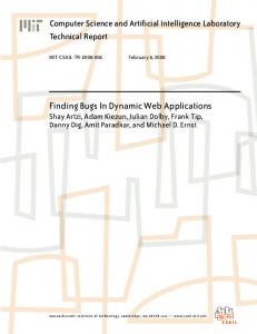
industries, so that various digital media applications offering the latest content are connected through communication networks, accessible from virtually anywhere. Increasingly, people expect to be able to access digital media applications through devices with a wide diversity in capabilities such as cell phones, PDAs, laptops and home entertainment devices, and they further expect to access them over a wide variety of execution conditions in terms of available bandwidth, total number of simultaneously running applications, amount of processing power, remaining battery energy, etc. Satisfying these diverse demands requires scalability, both in the digital media applications themselves in order to optimize the supplied content to the execution conditions, as well as in the application mapping in order to adapt to the conditions and to avoid running in power-hungry worst-case mapping modes, which is of extreme importance for wireless, low-power multimedia terminals. One way to obtain scalability in digital media applications is through the use of the Wavelet Transform (WT). The WT produces a mixed time-frequency, multi-resolution representation of a signal, inherently offering scalability. This is illustrated in Figure 1.1, which shows how 3 image resolutions can be extracted from an image transformed through a 2 level WT. By using this representation, it is possible to successively refine the resolution of the reconstructed signal (e.g. an image) using increasing subsets of the transformed signal. Aside from this resolution scalability, the WT can also be used in other types of scalability, such as distortion scalability, where larger subsets of the content stream lead to an improved signal-to-noise ratio (SNR) and temporal scalability, where larger subsets of video sequences lead to a frame rate increase. The complexity of these different quality modes scales orders of magnitude [Verdicchio 2004]. This should be taken into account when considering the mapping of the application to the device, in order to optimally adapt the mapping and minimize power consumption. This dissertation proposes a methodology for wavelet-based multimedia applications to achieve low energy use of the data memory hierarchy in embedded processors when faced with dynamically varying resource requirements. The methodology is based on adapting the application mapping to the encountered run-time conditions. This chapter starts by giving the corresponding problem formulation in Section 1.1. Section 1.2 gives a short overview of the Wavelet Transform, and motivates its importance by describing a wide range of fields in which it is used. Section 1.3 summarizes the main contributions of this work. Finally, Section 1.4 gives an overview of the structure of the dissertation.

1.1. Problem Formulation

3

Figure 1.1. Input Image, 2 Level Transformed image, and 3 resolutions corresponding to subsets of the transformed image.

1.1

Problem Formulation

Portable multimedia applications impose stringent and diverse requirements on their host platforms, as they should be energy-efficient for extended battery life, while simultaneously providing high performance. Many multimedia applications have huge data storage requirements, in addition to their pressing computational requirements. Previous studies show that high off-chip memory latencies and energy consumptions are likely to be the limiting factor for future embedded systems [Catthoor 1998b, Vijaykrishnan 2000]. Memory hierarchy design has been introduced long ago to improve the data access bandwidth to cope with the ever growing performance mismatch between processing units and the memory subsystem [Hill 1987, Patterson 1996]. Moreover, an SRAM-based domain or application specific memory hierarchy can be used to minimize the power consumption, as data memory power consumption depends primarily on the access frequency and the size of the data memory [Amrutur 2000]. Performance and power savings can therefore be obtained by accessing heavily used data from smaller Level 1 memories instead of from large power-hungry background memories. The Wavelet Transform (WT) produces a multi-resolution representation of a signal, forming an important but complex algorithmic component for a new class of scalable applications. In these applications it is possible to successively refine the quality of the reconstructed signal (e.g., a video sequence) by selecting increasing subsets of the transformed signal. This allows connecting heterogeneous systems to the same network with dynamically varying execution conditions, where each end-user can download a varying subset of the transformed signal and still achieve a reconstructed signal of optimal quality, according to the system’s technical capabilities and the encountered conditions. On the sys-

4


tem itself, the application will typically also have to deal with dynamism at task-level by competing for resources with other dynamically generated tasks with real-time constraints, meaning not only the amount of available signal content varies, but also these resources. Addressing this increased run-time dynamism will require new mapping strategies to deliver power-efficient performance. Fully static design-time mappings will not be able to optimally address the unpredictably varying application characteristics and system resource requirements. Instead, the freedom to dynamically scale the mapping requirements to the available resources can be exploited at run-time, so the battery life is adapted to these varying resources. Further energy savings can be obtained by also exploiting the freedom offered by reconfigurable systems and modifying the algorithm mappings to the changing system configurations, e.g. extra Level 1 memory can be activated under a sudden heavy work load [Balasubramonian 2003] and by exploiting the inherent scalability offered by wavelet-based applications in function of the user preferences, e.g. by indicating a user prefers a lower resolution representation of a video sequence over a reduced frame-rate version, or by indicating a user’s preference of seeing a complete low-resolution movie over half of the full-resolution sequence, if the projected remaining battery life suddenly decreases due to another task popping up. In this context, it is important for applications to optimally exploit the memory hierarchy under varying memory availability. This dissertation presents a mapping strategy for wavelet-based applications: depending on the encountered run-time conditions, it switches to different memory optimized instantiations or localizations, optimally exploiting temporal and spatial locality under these conditions. Obviously, this necessitates real-time mechanisms and mapping guidelines, derived at design-time and added to the middleware. This will be studied in this work through the parametric characterization of the WT miss-rate behavior for varying conditions.

1.2

Wavelet-based Applications

Wavelet-based coding is a powerful enabling technology for scalable applications, such as the JPEG2000 [Skodras 2001] and MPEG4-VTC [Sodagar 1999] compression standards and several similar proposed up- and downsampling schemes for scalable video coding in MPEG [Tran 2007, Ohm 1994]. Schemes coded by wavelet-based video coding have demonstrated that they can preserve excellent rate-distortion behavior, while simultaneously offering full scalability [Van der Auwera 2002, Woods 2001]. It is based on the principles of the Wavelet Transform (WT), a special type of subband transform [Woods 1991] producing a localized time-frequency analysis [Vetterli 1995], where the transform coefficients reflect the energy distribution of the source signal in both the space and the frequency domain.

5

1.2. Wavelet-based Applications

The following subsection briefly discusses the differences and similarities between the Wavelet Transform, the Fourier Transform and a related form of time frequency analysis, the Short Time Fourier Transform. It is followed by a summary of the historical development of the Wavelet Transform [Daubechies 1996]. Subsequently we describe how Wavelets are use to enable scalable coding and we finish this section by covering a range of specific multimedia and low-power signal processing applications based on the Wavelet Transform, to motivate why the WT is a representative and important building block for a wide range of applications.

1.2.1

Fourier Transform vs. Wavelet Transform

Amplitude

The Fourier Transform is a very useful analysis tool which can reveal information that is not directly visible in the time domain representation of a studied signal. By decomposing a signal in terms of sinusoidal basis functions of different frequencies, the signal is transformed into its frequency domain representation, allowing to analyze its frequency content and gain valuable insight in the structure of the signal. Figure 1.2 plots an example of a rapidly varying signal, whose Fourier Transform is shown in Figure 1.3. Through this frequency domain representation it is possible to derive that Figure 1.2 actually consists of a sum of two sinusoids.

Time

Figure 1.2. Stationary signal consisting of sum of two sines.

However, by transforming the signal into the frequency domain, the information about timing content is lost, since the signal is decomposed into sums of sinusoids, which have perfect compact support in the frequency domain but stretch out towards infinity in the time domain. For stationary signals such as the sum of sinusoids in Figure 1.2 this need not be a problem, but a lot of real-life signals are actually non-stationary, with spectral content that changes

6


Figure 1.3. The Fourier Transform of the signal in Figure 1.2 reveals its frequency content, consisting of two distinct frequencies.

over time and localized transient features such as discontinuities and edges.

Amplitude

Figure 1.4 gives an example of such a non-stationary signal, which intially clearly consists of one single sinusoid, replaced halfway by a sinusoid with a reduced frequency. Its Fourier Transform is shown in Figure 1.5, which is very similar to that of Figure 1.3. Therefore the sinusoid components of both figures have the same frequencies, but Figures 1.2 and 1.4 are visibly very different, and therefore the Fourier Transform does not clearly represent these differences between the signals. For a more complete picture, Figure 1.4 would benefit from a mixed time-frequency representation, as opposed to just a frequency representation.

Time

Figure 1.4. Non-stationary signal consisting of first a high-frequency sine and then a lower frequency sine.

Such a mixed time-frequency representation can be obtained through use of the Short Time Fourier Transform (STFT), which is based on first segmenting the signal by using a time-localized window and then applying regular Fourier analysis on each segment. If the frequency content of the signal then evolves

7


Figure 1.5. The Fourier Transform of the non-stationary signal in Figure 1.4 only gives information on global frequency content of signal. It is not distinguishable from Figure 1.3, even though their time domain signals are very different.

over time, it can then still be traced for each segment separately, thereby indeed offering a mixed time-frequency representation. The choice of the segmentation window determines whether there is a good time resolution, so that events can be localized well in time, or a good frequency resolution, so that frequency components close together can be distinguished. More formally, we can define ∆t and ∆ω for a window function centred on the origin in time and frequency respectively as R 2 t |ϕ(t)|2 dt 2 ∆t = R |ϕ(t)|2 dt R 2 ω |Φ(ω)|2 dω ∆ω 2 = R |Φ(ω)|2 dω ∆t and ∆ω can be seen as measures for the time and frequency resolution respectively, where a higher ∆t represents a larger window width and more uncertainty on the localization of events in the time domain, while a higher ∆ω represents a larger window bandwidth and more uncertainty on the localization of events in the frequency domain. A fundamental trade-off then exists in timefrequency analysis [Mallat 1998], which states that: 1 2 This is similar to the Heisenberg uncertainty principle, which states that it is not possible to measure both the position and the velocity of an object exactly at the same time. ∆t · ∆ω ≥

The choice of the STFT segmentation window then represents a compromise between the time- and frequency-based views of a signal. While the STFT

8


does offer information about both when and at what frequencies a signal event occurs, it can only offer this information with limited precision, and that precision is determined by the size of the window: for a wider analysis window the frequency analysis can be performed with increased accuracy, but the time resolution is reduced because it is smeared over the wide window. A narrow window can be selected instead to avoid this, but then the frequency resolution is simultaneously reduced. This is illustrated in Figure 1.6, where Figure 1.6c uses a narrow analysis window, so that time domain events such as switch points can be localized accurately, but at the same time the frequency resolution is sacrificed slightly. Figure 1.6d on the other hand uses a wider analysis window and therefore has a more accurate frequency resolution, but the position of time domain events get smudged in time and cannot be identified with the same accuracy. When analyzing real-life signals, it is often preferable to be able to locate features such as discontinuities, sharp peaks, edges accurately in time, but also to accurately identify the frequency content of slowly evolving components. This is where the Wavelet Transform comes into play, by offering good time resolution for high-frequency events, and good frequency resolution for low-frequency events. This is achieved by dilating or compressing the analysis window for different frequency bands, where compressed windows are applied for the high frequency bands and dilated windows for the low frequency bands. This effectively results in a different, non-uniform tiling of the time-frequency space or rather the related time-scale space, where the scale factor signifies the amount by which the analysis function is dilated or compressed, expressing information related to frequency content. Since the Wavelet Transform is governed by the same uncertainty principle as the STFT though, the total area of these tiles remains the same, as shown in Figure 1.6e. This different tiling leads to the Continuous Wavelet Transform, used as a powerful signal analysis tool in a wide range of applications. However, this representation has the drawback of being overcomplete and containing redundant information. In digital image processing applications, the time-scale space is therefore often subsampled using a specific subset of scale and translation values, in a manner which still permits perfect reconstruction.

1.2.2

History of the Wavelet Transform

Interest in the Wavelet Transform really took off in the 1980’s, after the work of a.o. Mallat and Daubechies lead to the widespread application in diverse fields such as image processing, computer vision, speech recognition, statistics and physics. However, the roots of the Wavelet Transforms can be traced back to several seemingly independent fields, long before that time.

9

Frequency

Frequency


Time

Time

b) frequency domain representation

Frequency

Frequency

a) time domain representation

Time

Time

d) Short Time Fourier Transform with higher frequency resolution

Scale

c) Short Time Fourier Transform with higher time resolution

Time e) wavelet domain representation Figure 1.6. Different representations correspond to different tilings of the timefrequency plane.

10


In essence, the idea behind Wavelet analysis is to decompose a signal f according to scale into a basis of functions Ψi : f=

X

ai Ψ i

i

This concept is related to the well-known Fourier Analysis developed by Joseph Fourier in the early 1800’s. He stated that any 2π-periodic, square integrable function can be represented by its Fourier Series consisting of a sum of sines and cosines: ∞ X f (x) = a0 + [ak cos(kx) + bk sin(kx)] k=1

In doing so, the time domain representation of the signal is transformed into a frequency domain representation, consisting of a decomposition into harmonics of different frequencies. In contrast to the fixed sines and cosines Fourier Analysis basis functions, an infinite set of basis functions are possible for the Wavelet Transform, which can in principle be adapted to the application properties.

φ(t) scaling function

0

1

t

ψ(t) mother wavelet (wavelet function) 0.5 0

1

t

Figure 1.7. Haar Transform Basis Functions.

In 1909 the first recorded mention of what came to be known as “Wavelets” could be encountered in the appendix of Alfréd Haar’s doctoral thesis. In the Haar Transform, a function is projected on to a set of orthogonal basis functions, specifically a scaling function with lowpass characteristics and squashed versions of the “Mother Wavelet” with bandpass characteristics, shown in Figure 1.7. The Haar wavelets are the simplest of the wavelet families, but their practical use is limited because they are not continuously differentiable, and they can therefore not quickly approximate smooth real-life signals. Nevertheless, Paul Lévy discovered in the 1930’s that the Haar transform was preferable above the Fourier transform for modeling the detailed behavior in Brownian motion, a type of random signal: due to the compact support of the Haar basis functions, they could more easily represent the small details present in Brownian motion, than was possible using the Fourier sinusoid basis functions which have infinite spatial support.


11

Related work on this shortcoming of the Fourier transform was performed by Dennis Gabor in 1946, leading to the Short Time Fourier Transform (STFT). In order to handle non-stationary signals where the frequency content changes over time, he proposed to first extract a signal segment using a time-localized window function. In this segment, the frequency content could be assumed to be stationary so that regular Fourier analysis could be performed on it. By shifting this window over the entire time domain, a mixed time-frequency representation is obtained in this manner. For the time-localized window function, Gabor selected a Gaussian function. Over the years, many variants on this concept were developed, mostly by changing the window function to obtain different trade-offs in time and frequency accuracy. The following major steps in the evolution of Wavelets were performed in the late 1970’s by Jean Morlet, a geophysical engineer working at the French oil company Elf Acquitaine. In applying standard and Short Time Fourier Transforms to analyze impulses sent into the ground during oil prospection to determine the thickness of underground oil layers, he found out that compressing or dilating a (Gaussian) windowed cosine gave a better trade-off in time-frequency localization. This process of dilating or compressing the basis functions is similar the Haar basis functions and stands in sharp contrast to the single fixed window used for the Short Time Fourier Transform. The term “Wavelet” also originates from this work: because this process resulted in small and oscillatory basis functions, Morlet referred to them as “ondelettes”, which translated into English became “Wavelets”. However, Morlet encountered difficulties convincing his fellow geophysics colleagues of the usefulness of his transform, due to the lack of a formal mathematical basis. Therefore he teamed up with Alex Grossman in 1980, a theoretical physicist with a background in quantum mechanics, who helped him develop a mathematically rigorous basis for his approach, as well as an exact inversion formula. In 1984, Yves Meyer, a French mathematician, noticed there was a great amount of redundancy in Morlet’s choice of basis, and set about developing an orthogonal wavelet basis with good time and frequency localization. Together with Stéphane Mallat, who came from a computer vision background, he developed the Multiresolution Analysis (MRA) construction for compactly supported wavelets in 1986. The MR construction allowed researchers and mathematicians to construct their own family of wavelets using its criteria. Furthermore, it made the use of Wavelets practical for engineering applications through the use of a simple and recursive filtering algorithm to construct the wavelet decomposition of a function. One drawback of Meyer’s orthogonal Wavelet bases was that their filters were of infinite length and required truncation for a direct implementation. In 1987 this problem was solved by Ingrid Daubechies by using filter design to develop

12


an orthonormal wavelet basis, instead of the other way around. This lead to a family of wavelets that, in addition to being smooth and orthogonal, were also compactly supported or zero outside a finite interval. In 1992, Daubechies cooperated with Albert Cohen and Jean Fauveau to construct the family of compactly supported biorthogonal wavelets. Relaxing the orthogonality requirement allowed greater flexibility in the construction of the wavelet filters so that it became possible to obtain nearly orthogonal Wavelets of perfect reconstruction with certain additional useful properties. Most notably this lead to linear phase filters of compact support, which is highly desirable in image processing applications to obtain convenient boundary extension schemes and especially to avoid visually disturbing edge distortion. The JPEG 2000 compression standard in particular uses the biorthogonal Daubechies 5/3 wavelet (also called the LeGall 5/3 wavelet) for lossless compression and a Daubechies 9/7 wavelet for lossy compression. Wim Sweldens proposed the lifting scheme in 1995 as a new method to construct biorthogonal wavelets, which did not rely on the Fourier Transform. Benefits of the lifting scheme include a more efficient calculation method by exploiting the similarities between the bandpass and lowpass filters, the freedom to use a fully in-place calculation method which doesn’t require any auxiliary memory, the straightforward generation of the inverse transform, the possibility to generate Wavelet Transforms mapping integers to integers and the ability to construct so-called second generation wavelets, which are not necessarily translates and dilates of one function and have applications such as irregular sampling and wavelets on curves and surfaces. This brief summary of the history of the Wavelet Transform illustrates that its roots originate from a fortuitous convergence of work in very diverse fields. This already suggests why the WT is so successfully applied in a wide range of applications. The following section focuses on how its multiresolution characteristics enable it to form the basis of scalable coding applications.

1.2.3

Scalable Coding

The work of Mallat [Mallat 1989] uncovered the link between Wavelet Theory and Multiresolution Analysis (MRA), which additionally resulted in an efficient procedure to calculate the DWT based on iterated filter banks. Figure 1.8 shows a schematic representation of the 1D multi-level Forward Wavelet Transform (FWT) procedure, whose outputs correspond to a sampled timescale space representation (Figure 1.10). The 1D WT can be generalized to a higher dimensional WT by interleaving the filtering in various dimensions during each level of the WT. The analysis filtering is first performed on each row of the input signal, and then on each column, before applying the necessary

13

1.2. Wavelet-based Applications subsampling operations and proceeding to the next WT level.

2

H

Input Stream

Level 0

L

2

HP 3

2

H H

LP n

2

L L

2

HP 2

2

HP 1

Level 1

Forward Lowpass Filter

Level 2

H

Level 3

Forward Highpass Filter

Level n

2

Subsampling

Figure 1.8. Forward Wavelet Transform Filtering Procedure.

The filtering procedure consists of a number of multiply-accumulate operations. The efficiency of this implementation procedure as a set of iterated filter banks has contributed to the success of the WT in many applications due to its conceptual simplicity: only one filter pair needs to be designed and the only necessary operations are (rather short) filtering operations. However, the iterative filtering combined with the subsampling typically leads to code with complex data dependencies and non-linear loop and index expressions, as is illustrated in Figure 1.9, where the row and column loopbounds scale exponentially in function of the WT level iterator. While it is feasible to remove these explicit non-linear loop and index expressions through code rewriting techniques, in this case by unrolling the WT level loop, this does not change the fact that the corresponding dependencies remain implicitly present in the code, since a level k sample will still depend on an exponentially increasing amount of samples from each lower WT level. This makes automated optimization strategies difficult to apply to wavelet-based applications, because they cannot suitably handle these non-linear dependencies and because the code unrolling techniques increase the complexity of the internal representation used in these strategies, making it difficult to find a good solution, as was shown for the automated memory hierarchy mapping tool MH in [Geelen 2006] and for the automated memory compaction tool in [Ferentinos 2005]. Each level of the FWT consists of a lowpass (L) and a highpass (H) filtering followed by a subsampling operation. The output of the lowpass filtering, after subsampling, represents the input to the next level of the transform, while the highpass samples are directly sent to the output and are not involved in the calculation of the successive FWT levels. The final output of an n level FWT is the result of the nth lowpass filtering (LPn) combined with all the highpass filtering results (HP1, HP2, HP3, . . . , HPn). The successive filtering

14


Figure 1.9. Pseudocode for the WT, showing complex index and loop expressions.

repeatedly halves the bandwidth of the intermediate signal, corresponding to the tiling of the time-scale space shown in Figure 1.6. As such, the complete Wavelet filterbank corresponds to a lowpass filter and a set of bandpass filters with constant relative bandwidth or ∆f = c(constant) f The output of the DWT is often organized according to the Mallat layout. Figure 1.10 shows this output organization for a 1D three level DWT and illustrates its relation to the sampled time-scale space; 0

31 INPUT

Scale

HP 1

DWT

HP 2 HP 3 LP 3

Time 0

8

4 LP 3

HP 3

31

16 HP 2

HP 1

DWT OUTPUT

Figure 1.10. 1D DWT Output of 32 samples in Mallat Organization.

Figure 1.11 shows an example of a 2D transformed image, as a hierarchy of subimages, grouped in levels according to the Mallat layout. Multiresolution

15


coding can be easily achieved by selective decoding of transform coefficients related to a certain frequency range or subband image. Other significant advantages of the WT for image coding compared to the widely adopted Discrete Cosine Transform (DCT), include high energy compaction (leading to large coding gain [Jayant 1984]), consistency with the human visual system (HVS) characteristics, and freedom from the common DCT blocking artifacts in the recovered images.

LL2 (DC) HL2

HL1

LH2 HH2

LH1

HH1

Figure 1.11. Input Image, 2 Level Transformed image, Regular Output Subband Organization.

A desirable feature for scalable compression systems is the ability to successively refine the reconstructed image. In this scenario, an approximation of the compressed data can be reconstructed after decoding only a small subset of the entire bitstream. As more of the bitstream is decoded, the reconstruction can be improved incrementally, until full quality reconstruction is obtained upon decoding the entire bitstream. Each part of the bitstream is itself a compressed bitstream, but at a lower rate (quality resolution). In this way heterogeneous systems can be connected to the same network, where each end-user can download only the amount of data corresponding to a desired resolution. The multiresolution representation of the WT complies with these requirements. Figure 1.11 (middle) and Figure 1.11 (right) respectively show a twolevel wavelet transformed representation and its generic output organization for the original IMEC building test image (Figure 1.11, left). The WT decomposes an input image into a hierarchy of subimages grouped in levels. The DC-image contains a low-resolution version of the original image, while the other subimages contain high-frequency information: the details needed to reconstruct the original image starting from the DC-image. In particular, the HLi , LHi and HHi maximally contain the details in the vertical, horizontal and diagonal direction of the original image respectively at resolution level i. This multi-resolution representation decorrelates the input image information, by packing the most relevant energy into a minimal number of pixels (the DCimage), while spreading “refinement” information through the different WT level subimages, with decreasing information relevance.

16


1.2.4

General Lifting Scheme

Though convolution based filtering architectures are possible for performing the WT operations, lifting based implementations offer certain advantages. The lifting scheme is a method for simplifying the WT by factorizing the filters into a set of prediction and update lifting stages [Sweldens 1995]. By exploiting the redundancy between the highpass and lowpass filters of the WT, this results in computationally more efficient implementations. Moreover, lifting scheme algorithms have the advantage that they do not require temporary arrays in the calculation steps, as the output of the lifting stage can be directly stored in place of the input. Therefore it has been applied in our experiments. In principle each of these lifting stages can themselves consist of different lengths, but we will restrict ourselves to 2 tap lifting filters. This configuration can be used to factorize all possible two channel, FIR subband transforms with perfect reconstruction, linear phase and least dissimilar length [Taubman 2002], which is of particular interest for image processing applications. KL

A

in

Lazy Transform (even/odd sample separation)

..ABAB..

... Prediction P1(z)

Update U1(z)

L out Prediction PK(z)

KH

B

...

Hout

1/KL

A

Lin

1/KH

Prediction PK(z)

Update U1(z)

Prediction P1(z) B

Lazy Transform (even/odd sample grouping)

Update UK(z) Hin

Update UK(z)

out ..ABAB..

Figure 1.12. Lifting implementation of wavelet analysis (encoding, top) and synthesis (decoding, bottom) filter [Sweldens 1995]

The generic lifting scheme consists of three types of operations: an initial lazy wavelet transform followed by prediction and update stages, as shown in Figure 1.12. The first step of the lifting structure is the so-called lazy transform, which splits the signal into its even- and odd-indexed components, and which on its own does not improve the representation of the signal. Therefore, the next step is to recombine these two sets in several subsequent lifting steps which decorrelate the two signal components. The two basic operations are prediction steps P (z) and update steps U (z), also referred to as respectively “dual” and “primal” lifting steps. A sequence of lifting steps consists of alternating lifts,


17

that is, initially the lowpass or even-indexed values are fixed and the highpass or odd-indexed values are decremented by the outcome of a lifting filter operating on the even-indexed values, while in the next step the highpass values are fixed and the lowpass values are incremented by the outcome of a lifting filter operating on the odd-indexed values. P (z) “predicts” the subsignal B, using subsignal A. If the subsignals are correlated, the prediction will usually be very good, so that subtracting the prediction from subsignal B will lead to a reduced correlation between the subsignals. Since subsignal B can then be reconstructed using this prediction error and subsignal A, we no longer have to store subsignal B, and the prediction error can be stored directly in-place of it. Meanwhile, subsignal A is updated to improve the subsignal properties (e.g. to avoid aliasing) with the filter U (z). In general, several such lifting steps can be applied in sequence. The number of lifting steps necessary as well as the values of coefficients in each step are determined by factorization of the equivalent wavelet filter pairs. Finally, normalization by factors KL and KH is applied. Moreover, two useful properties of the lifting scheme can be deduced from Figure 1.12: the inverse or synthesis transform can always be derived from the forward or analysis transform by changing the direction of the arrows, replacing the additions by subtractions and by inverting the normalization and lazy transform in the graph and it is possible to apply in-placing, by storing the output of each lifting stage directly in place of one of its inputs. For example, in the first lifting step subsignal B can be directly overwritten by the prediction error. Figure 1.13 illustrates that exploiting this in-placing freedom leads to interleaved distribution of lowpass and highpass samples. Furthermore, the repeated processing of the lowpass samples leads to exponentially separated lowpass samples at the higher levels. This fine grained and complex in-placing explains why automated in-placing optimization tools find it difficult to exploit this in-placing potential [De Greef 1998]. Nevertheless, it is not required to exploit this potential, since the outputs could just as easily be written to new arrays. Figure 1.13 shows a data-flow graph of the construction of the FWT by both successive filtering and lifting calculations through 3 wavelet levels, with a 5-tap lowpass filter and a 3-tap highpass filter and the equivalent lifting implementation, as applied in the JPEG2000 lossless mode. The lefthand side shows how lowpass values are computed using a 5-taps FIR-filter and the highpass values using a separate 3-taps FIR-filter. As shown on the righthand side, these same computations can be combined in the lifting scheme using two lifting stages, where initially the odd-indexed values are lifted in the first lifting stage using a 2-taps lifting filter operating on the surrounding even-indexed values, to produce a highpass value. Subsequently, the even-indexed values are lifted in the second lifting stage by a 2-taps lifting filter operating on the highpass values produced by the previous lifting stage. In general, each pair of filtering kernels of sizes 2n + 1 (lowpass) / 2n − 1

18


Figure 1.13. Forward Wavelet Transform Filtering and Lifting Operations.

(highpass) is decomposed into a set of Lift lifting stages with simple 2 tap lifting filters similar to the following pseudo-code: for (pos=0;poslevel)*colC+colF- colBUMP[L])/2] = … }

Figure 2.5. Partial block-based WT pseudocode illustrating complex, non-linear index expressions & loop structures.

Level 3 Level 2 Level 1 Level 0

0

1

x3...0

2

1 0

2 2

x2...0

3

2 0

4

3

6

7

5 8

9

x1...0 x0...0

8

10

12

16

14

18

10

11

10

11

20

22

Lowpass Samples Highpass Samples

5

6

7

10

12

14

Re-usable Memory Lowpass Filtering Highpass Filtering

16

Lowpass Data Dependencies Highpass Data Dependencies

Samples Previously New Input Stored into Memory Samples

Figure 2.6. Forward Wavelet Transform Data Dependencies.

2.3.2

Parallelization

As we will be specifically targetting locality trade-offs between different WT execution orders leading to corresponding memory hierarchy performance tradeoffs, we have thus far focused on memory related WT optimizations. Aside from this optimization field, a large body of work exists on exploiting parallelism, which can be considered complementary to our work. These works additionally apply a variety of the memory optimization techniques discussed in Section 2.3.1.

46

Chapter 2. Related Work

The Arquitectura y Tecnologa de Computadores (ArTeCS) group at the University of Madrid have extensively studied a number of topics on exploiting multilevel parallelism, specifically for the Wavelet-based JPEG2000 on General Purpose CPUs. These topics include SIMD parallelism exploitation [Chaver 2002, Chaver 2003], symmetric multithreading [Garc´ıa 2005], evaluation of functional pipeline splits and data level splits [Tenllado 2004a]. The parallelization of the WT on high performance supercomputers, as opposed to the General Purpose CPU approach of the ArTeCS group, is studied by [Nielsen 2000] which looks at different communication approaches for computing the horizontal and vertical filtering within a single level WT, while [Kutil 2000] extends this towards multilevel WTs and considers the trade-off between communication and recomputation. In recent years, interest has risen in using Graphics Processing Units (GPU) not only for 3D graphics acceleration but also for non graphics related applications, as their programmability increased, thereby offering the potential to exploit the massive parallelism they offer on commodity hardware. This General-Purpose computing on Graphics Processing Units (GPGPU) concept can offer significant speed-ups for data-parallel computational problems. In this context, [Wong 2007] applies the GPGPU concept to the WT computation and maps the RGB channels to 4 element GPU texels for additional SIMD exploitation, [Tenllado 2004b] uses a more balanced packing choice where selections of neighboring pixels in one channel are mapped to the GPU texels, while [Tenllado 2008] compares filtering and lifting-based WT implementations, where the filtering based implementations are more suited for the stream processing based GPGPUs. This is in contrast to traditional implementations where lifting based implementations are superior due to their reduced arithmetic complexity, and is related to the read-write dependencies between the lifting stages, which are problematic for the examined GPU platforms and programming model, so that the different lifting stages should be computed sequentially. The resulting reduced data locality compensates the effects of low arithmetic complexity of lifting-based WT implementations, making the filtering based implementation superior. However as GPU platforms are becoming increasingly more flexible and new programming models such as CUDA [NVIDIA Corporation 2008] are introduced, the constraints requiring sequential lifting stage computation can be expected to disappear.

2.4

Cache-oblivious Algorithms

[Frigo 1999] introduces a theory of Cache-oblivious Algorithms, representing algorithms where no variables dependent on hardware parameters such as cache capacity or line size need to be tuned to achieve optimality, and gives examples of such implementations for a number of algorithms such as matrix multipli-

2.4. Cache-oblivious Algorithms

47

cation, matrix transpose, and FFT. Cache-oblivious algorithms typically are based on a hierarchical divide and conquer principle, where the problem is repeatedly divided into smaller and smaller subproblems. Eventually, a subproblem size is reached which fits into cache, regardless of the cache size. Benefits of such cache-oblivious algorithms include simplification of porting towards other platforms and optimized performance on a memory hierarchy with different levels of cache having different sizes. The principle of a cache-oblivious algorithms contradicts our premise that different execution orders are optimal depending on the cache capacity. However, the theory of cache-obliviousness interprets optimality as asymptotic optimality, ignoring constant factors, so that further machine-specific tuning can be required. This is verified by [Olsen 2002], which implements a number of algorithms such as priority queues, and concludes that in practice the overhead incurred by making algorithms cache oblivious is too big for them to be competitive on all levels in the memory hierarchy.

48

Chapter 2. Related Work

Basic Switching Method Simulation Framework Mapping Guidelines

Temporal Locality

Intra-Task Dynamism

Chapter

3

Spatial Locality

New Layout Choices

Simulation Framework “I hear you’re buying a synthesizer and an arpeggiator and are throwing your computer out the window because you want to make something real. You want to make a Yaz record.” ‘Losing My Edge’ - LCD Soundsystem

This chapter presents our simulation flow and our architecture assumptions, based on which we develop the miss-rate characterizations for temporal and spatial locality in Chapters 5 and 6 and for intra-task data dependent behavior in Chapter 8. Section 3.1 describes the architecture template and characteristics. It shows how we can adapt to dynamically changing execution conditions, by switching between WT execution orders at run-time. Section 3.2 presents an extended reuse distance based simulator, which permits efficient analysis and characterization of the miss-rate behavior for a fully associative LRU cache, over all possible Level 1 sizes, despite the code and data dependency complexity present

49

50

Chapter 3. Simulation Framework

in the WT. Section 3.3 shows how to extend the characterization results generated using the extended reuse distance simulator for fully associative LRU caches towards other memory hierarchy systems. The chapter is concluded in Section 3.4.

3.1

Architecture Template On-chip

VLIW/DSP

Loop Buffers

Data-Cache Scratchpad (SRAM)

ARCHITECTURE TEMPLATE

Off-chip

Instruction Cache

VLIW/DSP

Loop Buffers

DMA

Data-Cache Scratchpad (SRAM) L1 Memory

Instruction Cache

Main Memory (SDRAM)

Peripherals

L1 Memory

Scenario Memory (Flash)

DMA

Figure 3.1. Architecture template used in this dissertation, including loop buffers.

Figure 3.1 shows our architecture template which consists of (multiple) VLIW or DSP processors, possibly with SIMD capability. The Level 2, or main memory is assumed to be off-chip Synchronous DRAM (SDRAM). Each processor possesses a private Level 1 memory. Typical sizes for the on-chip Level 1 memories in embedded systems are 2KB to 16KB. Modern embedded processors may further possess additional layers of on-chip memory. While this work focuses on architectures with one layer of on-chip memory, the techniques are extendable towards additional layers (see Section 4.1.7). The architecture also contains support for efficiently switching between implementations, in the form of small loop buffers and a non-volatile flash memory. The Level 1 data-memory can be either cache or scratchpad memory (SPM). In the embedded systems community, where energy and area are prime concerns, the SPM has lately gained prominence, in addition to the traditional cache. A SPM is essentially an on-chip SRAM that occupies a small part of the address-space of the main memory. The advantage of the SPM is that it is smaller in size and consumes less energy on a per access basis, because of its hardware simplicity: in [Steinke 2002] a factor 4 difference in energy per

3.1. Architecture Template

51

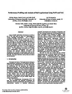
access is reported due to this overhead for a 4KB, 4-way set associative cache, compared to an equally sized SPM. Moreover, since it cannot be predicted beforehand when cache misses occur, a hardware-controlled cache is not suitable for embedded systems with hard real-time constraints. On the other hand, inserting a cache next to the SPM can also offer certain benefits, such as enabling the execution of applications ill-suited for SPM mappings, e.g. heavily unpredictable applications [Absar 2007]. Moreover, it is also possible to design intermediate reconfigurable schemes, e.g. where sets in a set-associative cache can be selectively configured as SPM [Texas Instruments 2004]. For a SPM the decision regarding which data should reside on it at any point in time is made in the application software. In this regard a SPM is significantly different from a cache, where this decision is made in hardware, typically by e.g. a least recently used (LRU) algorithm. In contrast, a SPM requires different (design-time) optimization techniques with increased emphasis on the energy reduction optimizations. Nowadays, these methodologies are implemented separately as source-to-source optimization frameworks. However, the complex data dependencies present in the Wavelet Transform make applying these methodologies in an automated manner difficult. On each of these processors multiple tasks will share the use of the processors and Level 1 space, to make more efficient use of these resources [Zhe 2006]. In this manner the processor idle time due to limited parallelism within a single task can be reduced, while varying resource requirements caused by application dynamism can be counteracted. These dynamically and unpredictably varying system resource requirements can arise from multiple sources. Tasks such as audio players and 3D visualization will pop up and get shut down at run-time. Moreover, the applications themselves will also present more and more dynamism. Complexity variations can result from multiple sources: content property changes, e.g. decoding of simple sea regions instead of complicated land regions in an image decompression application, dynamic user interactions leading to constantly changing running speed requirements, a scalable video coder which can switch to a lower quality video mode with a reduced resolution and frame rate, depending on the user’s wishes, the network conditions, etc. This will obviously result in different requirements being placed on the system architecture, as the processing requirements for these different modes can vary orders of magnitude [Verdicchio 2004]. If this dynamism is handled using static worst-case design strategies, the designs will typically be severely overdimensioned, making inefficient use of system resources. If the design is instead adapted to the encountered execution conditions, system resources will be exploited more efficiently and energy gains can be obtained. One way of doing this is by switching between different memory-optimized implementations or localizations of a 2D WT, which are more suited for specific Level 1 memory size ranges.

52


When dynamically introduced, pre-emptable tasks are present, especially in a multi-threading context, this Level 1 space can be traded off at run-time with other applications, meaning the amount of space varies over time and cannot be statically predicted. How the two execution orders behave when less (or more) Level 1 space is available than in the typical configuration, is different for both and results in a crossover point at smaller Level 1 sizes where e.g. the level-by-level localization performs better. This can be exploited at run-time by switching to the Pareto-optimal execution order for the encountered size, where Pareto-optimal signifies a solution is optimal in at least one trade-off direction, when all other directions are fixed. Figure 3.2 illustrates this for a 4 level forward WT of a 512 × 512 image, using the biorthogonal 9/7 wavelet filters, as employed in the JPEG2000 lossy mode [Skodras 2001]: it shows that for Level 1 sizes ranging from 20 bytes to 800 bytes the level-by-level execution order should be used, while for Level 1 sizes beyond 1KB the block-based execution order offers the best performance. The performance is compared using miss-rate as the evaluation metric. A miss tries to access data which is not present in Level 1 memory and which first needs to be fetched from costly L2 memory. A hit, in contrast, accesses data which is present in Level 1 memory [Patterson 1996]. This different behavior offers the freedom to dynamically scale the mapping requirements to the available resources so the battery life is adapted to these varying resources. Further energy savings can be obtained by also exploiting the freedom offered by reconfigurable systems and modifying the algorithm mappings to the changing system configurations, e.g. extra Level 1 memory can be activated under a sudden heavy work load [Balasubramonian 2003]. The mapping can then be adapted to this new configuration, by selecting a implementation with higher memory requirements, but significantly fewer misses. Obviously, this necessitates real-time mechanisms and mapping guidelines, derived by the compiler flow and added to the middleware. At design-time, the system can then be profiled to determine the most likely set of operating conditions or scenarios [Gomez 2002, Marchal 2003, Palkovic 2005], allowing the selection of a minimal set of different memory-optimized implementations. At run-time the middleware can then determine what the actual execution scenario is and, using mapping guidelines derived at design-time, switch to the most compatible localization, providing an optimized division of work over designtime and run-time. The mapping guidelines will represent a design-time characterization of the miss-rate behavior of different execution orders over a wide range of Level 1 sizes and for various algorithmic parameters, such as image size, filter size and number of WT levels, as will be derived in this dissertation. The run-time switching cost itself can be limited to a reasonable overhead using this characterization, even when multiple characterized tasks are present and the total available Level 1 space should be allocated between them in an optimized manner. This problem corresponds to the Multiple Choice Knapsack Problem

53

3.1. Architecture Template 7e+06

Block-Based Level-by-level

Missrate (loads and write backs)

6e+06

5e+06

4e+06

3e+06

52% 2e+06

18% 1e+06

0 10

100

1000

10000

100000

1e+06

1e+07

L1 size (bytes)

Figure 3.2. Relative miss-rate differences for 2 localizations of a 4 level, 9/7 filter WT.

(MCKP), which is known to be NP-hard [Martello 1990]. Nonetheless, the heuristic algorithm described in [Yang 2003] can find a good enough solution in as short as possible time, by exploiting the fact that the design-time derived configuration points are already Pareto optimal and ordered, i.e. it exploits the monotonicity of the curves, as opposed to the convexity of the miss-rate curves, which indeed they are not. Aside from the costs related to deciding whether and how to switch, costs related to performing the actual switching also exist. The costs of these other phenomena can be ignored, relatively speaking, if there is sufficient architectural support. This architectural support, illustrated in Figure 3.1, consists of small loop buffers for storing the program code of the relevant alternative implementations for one program phase, complemented by non-volatile (flash) memory for storing the program code of all possible implementation alternatives. The latter keeps leakage in the memory array fully under control. However, the periphery contains logic transistors that will still contribute to leakage in a very limited way [Samsung Electr. 2007, Snowdon 2005]. On the other hand it will exhibit a rather high read cost and a very high write cost, but this is compensated by the low access frequency: it is only written during program start-up or ideally even less, since it is non-volatile, which would also be beneficial for wear-levelling. In some cases, the flash program memory will be upgraded, e.g. based on a new downloaded version of code, but this will also happen extremely rarely, so it can be ignored. In addition, it is only read when a new program phase starts up, such as the 2D WT. For relatively predictable applications the loop-buffers can be filled by prefetching from this

54


flash memory, so that the switching delays can be ignored. The loop buffers themselves can be kept very small, due to the limited codesize for similar implementation alternatives [Palkovic 2007], and the inherent efficiency of small sizes for loop buffers, as shown in [Vander Aa 2005a], which shows an energy sweet spot for loop buffer depths between 32 and 128, for the Mediabench [Lee 1997] application suite. The switching frequency will depend on the different sources of dynamism. It will range from relatively low frequency switching due to events such as the end-user starting up new applications, selecting different configuration modes or variations in execution conditions such as battery capacity or network bandwidth, up to relatively high frequency switching related to events such as different motion scenarios within a video stream. According to [Yang 2003] an acceptable initial solution could be found in less than 12k cycles, which is 60 µs on a 200MHz processor. If we assume there would be 4 motion scenarios per frame at 30 frames/s, this would lead to 8.3 ms execution time per motion scenario, so that the switching time would amount to 0.7% of this execution time. Moreover, this would assume that during each frame a re-allocation of Level 1 space due to the introduction of new motion scenarios was required, whereas in reality this is likely to be lower, if the motion scenarios in a future frame could be predicted based on those present in the current frame.

3.2

Simulation Framework

The simulation framework used in this work to derive the design-time characterization of the miss-rate behavior is based on the concept of reuse distance [Beyls 2002], a metric expressing locality. In this section we first give the definition of reuse distance and how it relates to the notion of stack simulation [Mattson 1970]. Then we describe how the simulator has been extended to take the cost of write backs into account, and to aid in visualizing the reuse distance, which is helpful for the characterization of the miss-rate behavior. We conclude by briefly describing how generalized Wavelet Transforms were generated, used as inputs for the simulator.

3.2.1

Reuse Distance Simulator

The following definitions are used [Beyls 2004]: Definition 1. A memory reference corresponds to a read or a write in the source code of a program, while a particular execution of that read or write at run-time is called a memory access. A reuse pair is a pair of accesses

55

3.2. Simulation Framework

to the same data location without intervening accesses to that location. The use of a reuse pair is the first access, the reuse is the second access. The reuse distance of a reuse pair is the number of unique data locations accessed between use and reuse, or more formally, for two read accesses xr (t1 ) and xr (t2 ) to the same address x in the memory address space MA, at times t1 and t2 , the reuse distance (RD) can be defined as [Vander Aa 2005a]: RD(x)(t1 , t2 ) := #{y ∈ MA | ∃ y(t) and t1 < t < t2 } Definition 2. The backward reuse distance (BRD) of a memory access is the reuse distance of the reuse pair in which this access is the second access. If the element is accessed for the first time no such pair exists and the BRD is defined as ∞. Figure 3.3 illustrates this for a short reference stream. Note that the reuse distance for the final access to A here is equal to 3 instead of 4, because the reuse distance corresponds to distinct locations accessed.

t1 A

X

Y

3

Z

t2 A

V

W

X

Y

Z

t3 A

V

W

5

V

X

t4 A

3

Figure 3.3. Reuse Chain for Reads to Element “A”.

In [Beyls 2002], it is proven that for a fully associative cache with n entries and least recently used (LRU) replacement policy [Hayes 1988], an access with a reuse distance r < n will hit, while an access with reuse distance r ≥ n will miss. This implies there is a one-to-one relation between the miss-rate of a fully associative cache of a certain size n and the sum of all accesses with reuse distance r > n. This sum of all accesses can be obtained by using a reuse distance histogram. The cumulative histogram then represents the total hit-rate, or the total accesses − miss-rate. For the references to A in Figure 3.3 the reuse distance histogram contains two accesses at distance 3, one at 5 and 1 at ∞, so that for a cache size ≤ 3 all accesses will miss, for cache sizes ≤ 5 just 2 accesses will miss, and otherwise only the first access will miss. All these reuse distances can be computed as the depth of an access in a LRU stack, which is related to the concept of stack simulation, first proposed by [Mattson 1970] in the context of page replacement in virtual memory systems. Stack simulation allows single-pass, trace-driven simulation of many alternative caches, subject to the same stack replacement algorithm. In order to simulate the miss-rates for multiple cache sizes, a possible procedure could

56


consist of executing a different simulation pass for each cache size. Such a brute force simulation would determine the cache contents at any time t and would keep track of the number of times an access could not be resolved by the cache, leading to a cache miss. As such it would have to count the cache miss-rates separately for each separate size. A greatly simplified method for deriving the miss-rate over a wide range of cache sizes can be obtained from certain properties of the replacement function, i.c. the LRU replacement function. After accessing at least C distinct data elements, a cache of size C will contain the C most recently used elements. When a new element is addressed, this element replaces the least recently used element present in the cache, so that at that particular time the cache still contains the C most recently used elements. In fact, for all possible access traces and cache sizes C, the contents of the cache at a particular moment t may be derived by by scanning backwards from point t in the trace and collecting the first C distinct elements encountered. Since the set of C most recently referenced distinct elements is always contained in the set of C + 1 most recently referenced distinct elements, the contents of a cache of size C will be a subset of the contents of a cache of size C + 1. This is referred to as the inclusion property: at any instant, a larger cache always contains all the data in all smaller caches. Because of this inclusion property the cache contents at any time and for any cache capacity can be represented by one single LRU stack, containing an ordered set of all encountered accesses, ordered along the time of least recent use, meaning the most recently used element is stored at the top and the least recently used element is stored at the bottom. In general, this inclusion property should hold in order for stack simulation to be possible for other replacement policies, so that one single simulation pass can be used to simulate all possible cache sizes for these other replacement policies. The sequential list-based search of this stack may form a bottleneck in stack simulation. The simulator of [Beyls 2004] therefore computes the full histogram of reuse distances more efficiently using a random treap representation of a LRU stack, which is a data structure combining a tree and a heap, that orders the nodes by adding a random priority attribute to a node, as well as a (LRU counter) key. The nodes are ordered so that the keys form a binary search tree and the priorities obey the max heap order property, so that on average the binary search trees are balanced thanks to the use of the random priorities [Seidel 1989].

3.2.2

Write Back Extension

The simulator makes no distinction between read and write accesses, and therefore does not accurately consider the cost of write accesses. In order to improve the accuracy of the simulation results and to permit a fair comparison to the

3.2. Simulation Framework

57

existing scratchpad based mapping tools, the simulator has been extended to take write accesses into account. Multiple write policies are possible, where the most significant simulator changes are required for a write back policy. For this policy, the data is only written back to the main memory when it is evicted from the cache, to avoid unnecessary write backs. For this purpose, a status bit is commonly used, called the dirty bit, indicating whether the block is dirty (modified while in the cache) or clean (not modified). One option to simulate the write back cost is by explicitly using these dirty bits. After each write access, the addressed data becomes (or stays) dirty and will suffer a write back upon eviction. Moreover, if the write access misses, there can additionally be a load miss, depending on the applied policy. We typically assume a fetch-on-write-miss policy. For the read accesses, a hit will not modify the status of the dirty bit, whereas after a miss the status must be clean, as the data would have already been written back upon a previous eviction. An issue here is that the moment of eviction is cache size dependent, and therefore we cannot simply add clean or dirty flags for each element, since their value would also depend on the cache size. Instead, the cost of write backs can be modeled by using the concept of a maximal write distance, which exploits the fact that these flags do change in a systematic manner: once a particular element A has been written to, its status becomes dirty. Afterwards, as it moves through the LRU stack due to accesses to other elements, it will cause write backs for increasingly larger cache sizes. Right before being accessed again, it will have reached a maximal distance inside the LRU stack. Therefore it will cause write backs for all caches with a size lower than this corresponding distance, called the write distance. If the subsequent access to A is again a write, it will overwrite the previous value, so that that particular value or corresponding write operation will only be written back for cache sizes below the write distance. This means we can add an access to the write distance histogram at that distance. However, if the subsequent access to A is a read, the element will remain dirty, and may afterwards move even further through the LRU stack, to an even higher distance. Accordingly, we should not simply insert the write distance directly after a write access into the reuse distance histogram, but we should actually insert the maximal write distance, in between two subsequent write accesses. The method described above is similar to the work in [Thompson 1989], but it has been independently developed. For two consecutive write accesses xw (t1 ) and xw (t2 ) to the same address x at times t1 and t2 , the write distance (WD) can be formally defined as follows: W D(x)(t1 , t2 ) := max{BRD(t) | ∃ xr (t) and t1 < t ≤ t2 } The concept is illustrated in Figure 3.4. The access at t1 is a write access, making the considered element A dirty and

58

Chapter 3. Simulation Framework Read Access

t1

Write Access

t2

Reuse distance

t3 5

3

Maximal write distance

5

END

t4 3

3

10

10 or

Figure 3.4. Read and Write chain for element A.

causing a maximal write distance of 5, until the following write occurring after two arcs with reuse distances of respectively 3 and 5. This means A will have travelled the LRU stack to a distance of 3 before the second (read) access, and to a distance of 5 before the second write access at t3 , implying that for caches ≤ 3 the eviction and corresponding write back will occur during the first arc, while for cache sizes of 4 or 5 the write back will occur during the second arc. However, this has no impact on the total write back costs and the write distance histogram: if the cache size ≤ 5, this first write access will have been written back. If the cache is larger than 5, A will have been over written again, thereby avoiding the first write back. The write at t3 will then simply be written back if the cache size ≤ 3. The final write access at t4 will either always be written back (if the cache is flushed at the end), or it will be written back for cache sizes ≤ 10, assuming 10 distinct locations will have been accessed before the end of the stream, after this write. To compute this, it is sufficient to add a maximal backwards write distance to each node representing a data element in the LRU stack. The reuse distance histogram for read accesses can simply be computed in the traditional manner: each time a read occurs the data element is brought to the front of the LRU stack and the reuse distance histogram is incremented for the distance that the data element was originally positioned at in the LRU stack. Furthermore, if the element has ever been written to, this distance should be compared to its stored maximal reuse distance, replacing it, if it is larger. After the first write access to an element, the element is identified as having been written to. The maximal reuse distance is once more updated, the node is moved to the front of the stack and if there is a fetch-on-write-miss policy, the reuse distance histogram is incremented as if the access were a read. Finally, the maximal write distance is also inserted into the write distance histogram and the maximal reuse distance of the element is reset to 0. For the final write backs, the entire LRU stack should be traversed to find the elements which have ever been written to. For each of these elements the write distance histogram is either incremented at ∞ (if the cache is flushed and the final write back can therefore not be avoided) or at the final distance of those elements in the stack. Finally, if a write through policy is desired instead of write back the reads may

59

3.2. Simulation Framework %Reuse Distance Misstrace: %Location Source Line Tag %------------------ --input[0][0] 50 wb input[0][0] 50 wl input[0][1] 102 r input[0][0] 102 r input[0][2] 102 r input[0][1] 104 wb input[0][1] 104 wl input[0][0] 112 r input[0][1] 112 r input[0][1] 112 r input[0][0] 114 wb input[0][0] 114 wl input[0][3] 102 r input[0][2] 102 r input[0][4] 102 r input[0][3] 104 wb input[0][3] 104 wl

Reuse Distance -------------First Write Compulsory Miss Compulsory Miss 1 Compulsory Miss First Write 2 2 1 0 2 1 Compulsory Miss 3 Compulsory Miss First Write 2

Figure 3.5. Miss-trace extract from the start of a WT

be processed as usual, while for writes the write distance histogram is always incremented at ∞, as these writes occur regardless of the cache size.

3.2.3

Characterization Extensions

The simulator has additionally been extended to dump miss-traces and visualize access footprints, to help in the characterization and formalization of the missrate behavior. A miss-trace consists of the original access trace, annotated with the encountered reuse distance for each access. It is dumped by the simulator while performing the reuse distance analysis and updating the reuse distance histograms. To further aid in the interpretation, each address is translated back to the corresponding array location and tags distinguishing between reads, write loads or write backs are included in the miss-trace, as well as the line in the source code where the access is performed. Figure 3.5 shows a short extract from the beginning of a trace for a fully in-placed WT. As the extract is limited to a short fragment from the start of the trace, all of the illustrated reuse distances are quite low. By searching the trace for specific occurrences of larger distances, it helps determine which reuse mechanisms contribute to miss-rate drops at specific Level 1 sizes. The miss-traces can further be used to visualize why these reuse mechanisms

60


occur at a particular size. For a specific occurrence of a reuse distance in the miss-trace, this is achieved by dumping an image marking all distinct samples accessed between the use and reuse of a reuse pair representing the access footprint of the data contributing to the targeted reuse distance. Figure 3.6 illustrates this for 4 reuse distance points on block-based and level-by-level missrate curves of a 9/7 filter, 4 level in-placed WT. The first two points correspond to the block-based localized execution order. After zooming in on the images, the first size is revealed to correspond to only a small number of locations, while the second point shows a complicated access pattern over the entire width of the image and represents the size required to exploit all possible block-based reuse. The final two points are located on the level-by-level curve at relatively large sizes. On the image the actual reuse location itself, representing a specific access in the miss-trace with the targeted reuse-distance, is highlighted in light gray. The actual reuse mechanisms and the link to the execution orders will be further explained in Chapter 4 and formalized in Chapter 5. A final visualization extension added to the simulator helps analyze the spatial locality effects. The second and third points in Figure 3.6 show a varying distance between many of the samples in the access footprint, leading to a reduced spatial locality for these samples. When visualizing the access footprint, in addition to plotting the samples directly accessed, it is also possible the show those samples which are located on the same cache-line as directly accessed samples in the footprint. When data is loaded from the memory, a complete line is always brought into the cache, and therefore these samples are also fetched and stored. This is illustrated in Figure 3.7 for the maximal reuse point of the block-based execution order of Figure 3.6, when the line size is increased from 1 to 4 words/line. In Chapter 6 this is used to formalize the impact of spatial locality on the miss-rate behavior.

3.2.4

Source Code and Trace File Generation

Since the simulator uses access traces as inputs to produce the reuse distance histograms, the miss-traces and the access footprint visualization, there should be a way to produce these access traces for WTs under varying algorithmic parameters. For this purpose, scripts are used to generate source code for various WT instantiations, which are instrumented, using ATOMIUM analysis [IMEC 2006], to generate access traces of array references. It is assumed that only the array references generate memory accesses. WT filters of different length, based on lifting implementations, are simulated by concatenating multiple lifting stages composed of 2 tap lifting filters, as in the pseudo-code below: for (pos=0;pos Ea ): Eb − Ea Eb

= = =

(EL1 + EL2 ) · (missb − missa ) EL1 · (accessestotal ) + (EL1 + EL2 ) · missb missb − missa 1 × accessestotal L1 missb 1 + EL1E+E missb L2 missb − missa ×τ missb

(4.1) (4.2) (4.3)

When converted to a relative gain in energy, a gain in miss-rate is reduced by the translation factor τ given in equation 4.3 above. It indicates that when the miss-rate is relatively low and EL2 is not much higher than EL1 , most of the gains related to the miss-rate reduction are hidden by the constant EL1 · accessestotal in the energy formula. However, in a good memory hierarchy design for embedded applications, the total energy consumption is reduced by making EL1 low, requiring small Level 1 sizes. The Level 2 size and the corresponding EL2 will then be much larger, as it still needs to be large enough to store large data in background. In such cases, the translation factor τ is close to one, even for small miss-rates, and a reduction in miss-rate translates directly to a reduction in energy. Table 4.1. On-chip SRAM energy [Papanikolaou 2003]

size (bytes) energy (nJ/access)

1024 0.024

4096 0.045

8192 0.068

65536 0.311

131072 0.473

1048576 1.894

Table 4.2. Off-chip SDRAM energy (Micron MT48LC16M8A2, [Micron 1999])

energy (nJ/access) energy (nJ/page activate)

3.5 10

According to the energy numbers given in table 4.1, an 8 kB Level 1 SRAM memory has an energy cost of 0.068 nJ/access, while according to table 4.2 if we assume 20% page misses, a 128 MB Level 2 SDRAM memory on average leads to an energy cost of 3.5 + 0.2 · 10 = 5.5 nJ/access. For these energy costs, and with the miss-rates given in Figure 4.11, the translation factor τ for the miss-rate reduction of 18% is 95.3%, leading to an energy gain of 17%, while for the miss-rate reduction of 52%, τ is 97.7%, giving an energy gain of 51%. This shows that within the embedded multimedia and wireless context, these miss-rate reductions indeed lead to nearly proportional energy reductions. These two miss-rate gains are plotted on Figure 4.18, which shows how the translation factor τ evolves in function of the energy ratios EL1 /EL2 and the miss-rate ratios missb /totalaccesses .

88

Chapter 4. Basic Switching Method

Note that if there is further also an on-chip Level 2 memory, this will typically be in a size range of 128 kB to 1MB. For those kinds of large sizes, the memory layers will become more costly to access in terms of energy, resulting in a smaller energy-per-access difference between Level 2 and the off-chip memory. Consequently, the translation factor will decrease, so that the miss-rate differences will translate to smaller energy differences. However, even for a EL2 of 1MB and the miss-rate reduction of 18%, the corresponding translation factor of 50% (cf. Figure 4.18) will still result in an energy reduction of 9%. τ = 60%

τ = 50%

0.5

τ = 70%

0.4 Large L1,18% miss-rate gains

τ = 80% EL1/EL2

0.3

0.2

τ = 90% 0.1

Small L1,18% miss-rate gains

τ = 95% τ = 97.5%

Small L1,52% miss-rate gains

0 0.2

0.3

0.4

0.5

0.6

0.7

0.8

0.9

1

missb/totalaccesses

Figure 4.18. Required energy ratios EL1 /EL2 in function of miss-rate ratios missb /totalaccesses , for different values of the translation factor τ

In a static environment, a designer knows how much Level 1 space is available and can choose a suitable execution order. As level-by-level is only optimal for quite limited Level 1 sizes, a block-based execution order will be chosen typically. In a dynamic environment we cannot predict at design-time how much Level 1 space is available. We can then either keep only the block-based execution order, which will have an optimal miss-rate most of the time, or we can switch to a level-by-level execution order when there is a heavy workload and Level 1 space becomes limited. If we assume enough memory for the block-based execution order is available 80% of the time, switching over to the level-by-level execution order in the remaining 20% would still deliver a 19% energy saving, compared to always staying in the block-based execution order, if the run-time switching energy overhead costs may be ignored. The SRAM and SDRAM energy figures given in table 4.1 and table 4.2 can also be used to give an idea of the run-time switching energy overhead costs, by

89

4.2. Energy Gains Due to Switching

comparing the orders of magnitude of the energy consumed by the switching strategies in the instruction memory hierarchy, to the energy savings obtained in the data memory hierarchy, keeping in mind the architecture template shown in Figure 3.1. This shows architectural support for efficiently performing the switching, consisting of small loop buffers for storing the relevant alternative implementations’ program memory, complemented by non-volatile flash memory used for storing the program code of all possible implementation alternatives. (a) 32 bits wide, 64 rows high, umc90 technology loop buffer [Raghavan 2008]

energy (nJ/activation) leakage power (µW )

0.00943 9.19

(b) NAND flash ory, [Samsung Electr. 2007]

page read (nJ/512 bytes) page write (µJ/512 bytes) standby power (µW )

mem-

171 1.98 18

Table 4.3. Energy consumption of loop buffers ((a)) and flash memory ((b))

For the loop buffers, we assume that one is used per scenario, with a width of 32 bits and a height of 64 rows. This is well inside the optimal specifications of 32 to 128 rows mentioned in [Vander Aa 2005a], and will lead to a dynamic cost of 0.00943 nJ/activation and a leakage power of 9.19 µW (table 4.3(a)). For the flash memory, a page read incurs an energy consumption of 171 nJ/512 bytes, a page write suffers an energy consumption of 1.98 µJ/512 bytes and the standby power consumption is 18 µW (table 4.3(b)). Since the flash memory is written very infrequently, in principle even less than once per program activation, the high page write cost can be ignored globally. Flash memory read accesses, on the other hand, will occur more often: in order to reduce the switching time overhead for relatively predictable applications, the loop-buffers can be filled by prefetching from this flash memory each time a new program phase with new scenarios occurs. If 8 complete loop buffers should be filled in this manner, this amounts to a flash memory read cost of Eflash,r = 171 nJ/512 bytes · 256 bytes/loop buffer · 8 loop buffers = 684 nJ and a corresponding loop buffer write overhead cost of Eloop buffer,wr = 8 loop buffers · 64 rows · 0.00943 nJ/activation = 4.83 nJ Likewise, if there are 8 scenario changes during a program phase, and an entire loop buffer should be read each time, an energy cost occurs of Eloop buffer,r = 8 changes · 64 rows · 0.00943 nJ/activation = 4.83 nJ In total this amounts to a cost of 693.66 nJ per program phase. To approximate the leakage energy during a program phase, we examine the contributions of the flash memory and of the loop buffers. In order to calculate

90


the leakage energy of the loop buffers, we will use the above-mentioned figure for the leakage power, multiplied by the time of the program phase. Beyond that phase, the buffer and the associated logic can be cut off from the power supply by power gating, so that no leakage occurs any more. To compute the leakage contribution, we can use a very rough approximation of the execution time, attributing 2 cycles to a data access and 1 cycle to an arithmetic operation. For the WT parameters of Figure 4.11 on a 200MHz processor, this leads to TW T

=

512 rows · 512 cols · 2 dims · 1.33 Level scaling · 4 Lifting stages (2 · 4 accesses + 3 operations)/200 MHz = 0.1532 sec

or a leakage energy of: Eleakage,loop buffers = 8 loop buffers · 0.1532 sec · 9.19 µW = 11.26 µJ The standby energy of the flash memory is similarly evaluated as: Eleakage,loop buffers = 0.1532 sec · 18 µW = 2.76 µJ This execution time approximation is very coarse, and ignores factors such as ILP, loop buffer shutdown and cache misses, but we are primarily interested in its order of magnitude, to compare the corresponding leakage cost to the data memory energy savings. The sum of the dynamic and static switching costs is equal to 14.7 µJ. Using the 2D WT as an example of a program phase, we can reuse the energy figures of tables 4.1 and 4.2 to calculate the total data memory energy gains during this program phase. The energy consumed during normal operating conditions amounts to Enormal

= 0.068 nJ/L1 access · 6963200 total accesses + (0.068 nJ/L1 access + 5.5 nJ/L2 access) · 1432776 misses

= 8.451 mJ

The energy consumed during peak conditions, respectively without switching and with switching (to the level-by-level execution order), can be computed as Epeak,no

switch

= 0.068 · 6963200 total accesses + (0.068 + 5.5) · 3649475 misses

= 20.793 mJ Epeak,switch = (0.068 + 5.5) · 1740800 misses =

0.068 · 6963200 total accesses + 10.166 mJ

4.3. Miss-rate Trade-off Requirements

91

If peak conditions occur 20% of the time, the total amount of energy saved by switching then amounts to: ∆switch

= (a · Enormal + (1 − a) · Epeak, no switch ) − (a · Enormal + (1 − a) · Epeak, switch ) = 2.1255 · 106 nJ = 2.1255 mJ

Compared to the combined dynamic and static energy cost of 14.7 µJ, these overhead costs are only 0.7% of the total savings, indicating they can indeed be ignored, even if the static energy consumption calculation is quite coarse. These principles will potentially need to be adapted when reconfigurable architectures are considered or for unpredictable applications, where future work will be needed to enable the mapping guidelines to evaluate the impact of e.g. the energy and timing cost of activating extra Level 1 memory or the timing overhead of scenario code transfers, when this cannot be hidden by prefetching in unpredictable applications.

4.3

Miss-rate Trade-off Requirements

The previous section demonstrated how the relative miss-rate differences found between different WT execution orders can translate to memory transfer energy gains. This section covers what the requirements are to encounter these missrate differences for different execution orders. For this purpose, the proposed JPEG XR still-image compression standard and the Cavity Detector medical image segmentation application are used to illustrate when miss-rate trade-offs can occur.

4.3.1

JPEG XR

JPEG XR is a recent JPEG proposal [JPEG 2007], based on Microsoft’s HD Photo [Srinivasan 2007]. It offers many similar features to JPEG2000 at significantly reduced complexity, but with reduced flexibility. The compression performance is still under investigation, with the first results suggesting it is typically worse than JPEG2000 and better than traditional JPEG [De Simone 2007]. It offers resolution scalability and as such it is an interesting multi-resolution candidate to check whether the localization switching principles also apply here. In contrast to the JPEG2000 filtering based system, the HD photo hierarchical system is block-based with each 4 × 4 sample input block within a 16 × 16 macroblock undergoing a first stage transform, producing 1 DC coefficient and 15 AC coefficients as outputs for each of the 16 blocks within the macroblock.

92


Similar to the Wavelet Transform, the 16 DC coefficients are then further transformed in a second transform stage, after being collected into 1 single 4 × 4 block, ultimately leading to 1 Level 2 DC coefficient (“DC ”), 15 Level 2 AC coefficients (“Lowpass”) and 240 Level 1 AC coefficients (“Highpass”). This implies the resolution scalability is algorithmically limited to 3 resolutions, with a downscaling factor of 4. In contrast, JPEG2000 has more flexibility in its resolution scalability, with a downscaling factor of 2 and a limit on resolution levels which is only determined by the input image size, and not by a hard algorithmic constraint. Each of the two transform stages is constructed as a flexible concatenation of two different block-based transform operators: Photo Core Transform (PCT) and Photo Overlap Transform (POT). PCT is similar to the widely used discrete cosine transform (DCT) and can exploit spatial correlation within the block. However, PCT has some of the same shortcomings as DCT and other block transforms in that it cannot exploit redundancy across block boundaries and can result in blocking artifacts at low bitrates. Therefore, POT is intended to exploit the correlation across block boundaries as well as to reduce blocking artifacts and thus address the drawbacks of PCT. The PCT is always performed, at each transform stage. However, there are 3 options for controlling the POT: disabled for both stages, enabled for the first stage but disabled for the second, and enabled for both stages [Srinivasan 2007]. Figure 4.19 is a top-down view showing how these operators cause similar exponentially increasing dependencies as the WT, both without and with the presence of the optional POT operator. In the first case a macroblock of 16 × 16 samples is needed to directly produce 1 sample at the highest resolution, while in the second case, due to the overlap operator, a much larger size of 36 × 36 samples is required, overlapping similarly to the dependency bands of the WT. Furthermore localization transformations can be applied in both cases, but in the first case only those misses related to the second PCT will be avoided or about 1/16 of the total misses. This is less than in the WT because the 2D WT has a downscaling factor of 2 instead of 4 and it has horizontal and vertical dimensions of filtering, whereas JPEG XR applies block-based processing instead. In the second case with the POT operator, the misses between POT1 and PCT1 can also be avoided. Therefore localization makes more sense then. Figure 4.20 illustrates the miss-rate behavior for a simulated PCT/POT chain. The localization indeed offers a useful 22% miss-rate decrease, but there is no miss-rate trade-off: the localized execution order always offers a superior or equal performance. It still needs a relatively large Level 1 size to exploit the inter-level reuse, but in contrast to the WT, this does not translate to a worse miss-rate if these Level 1 size requirements are not met. This is not the case for the WT, where at small Level 1 sizes the localized

93

4.3. Miss-rate Trade-off Requirements

PCT1

PCT2

(a) No POT.

PCT1

PCT2

POT2

POT1

(b) With POT.

Figure 4.19. Multi-resolution analysis in JPEG XR.

execution order fails to exploit not only the inter-level reuse, but also a large part of the filtering reuse within each WT level due to its irregular execution order, whereas the level-by-level execution order still manages to exploit this filtering reuse at these small Level 1 sizes. However, since JPEG XR works on a block-basis, there is no reuse source similar to the filtering reuse, which level-by-level can exploit and localized cannot. Indeed, at low Level 1 sizes, we need to ensure that a block still fits. If it fits, the intra-block reuse can be exploited, but it can be exploited by both execution orders. If a block does not fit, neither execution order can exploit the intra-block reuse. In fact, to have a miss-rate trade-off between different localizations, there should also be a reuse source trade-off, where exploiting more of a particular type of reuse at a particular size, means exploiting less of another type of reuse at a lower size. In a block-based localized WT different WT levels are merged within a dependency pyramid, to move the inter-level reuse to smaller Level 1 sizes, but this also moves the filtering reuse to larger Level 1 sizes.

94

Chapter 4. Basic Switching Method 1e+07 Level by level Localized

Missrate (bytes)

8e+06

6e+06

Reuse within blocks exploited

Scale 2 arrays fit

Scale 1 arrays fit

22%

4e+06

2e+06

0 1

10

100

1000

10000

100000

1e+06

1e+07

L1 size (bytes)

Figure 4.20. Missrate behavior for JPEG XR using level-by-level and localized execution orders.

4.3.2

Cavity Detector

A similar reuse trade-off can be observed in the Cavity Detector application. Cavity detector is an image processing algorithm for the segmentation of medical images consisting of a pipeline of processing stages [Deklerck 1993]. These multiple processing stages (horizontal filtering, vertical filtering, edge detection, root labeling) can also be merged together, similar to the WT resolutions. By merging the processing stages the size required to exploit the reuse between the stages shift towards smaller line-buffer-based or kernel-based sizes. At the same time other sources of reuse are shifted towards larger Level 1 sizes, such as the vertical filtering overlap reuse which shifts towards larger line-buffer sizes and the horizontal overlap reuse which shifts towards merged kernels for all processing stages. The resulting miss-rate trade-off is shown in Figure 4.21. The reason why multi-resolution analysis is interesting in the context of missrate trade-offs, is that the sizes required for merging grow exponentially with the number of resolution levels due to the downsampling dependencies, complicating the analysis and ensuring that the trade-off is likely to occur over an extended Level 1 range. In contrast, if only a few horizontal kernels are merged, the size required for this merged kernel-group is likely to be limited, so that

95

4.4. Conclusion

Unmerged

1.4e+07

Fully merged 1.2e+07

Missrate (words)

1e+07

8e+06

6e+06 35,5%

4e+06

2e+06

37,5%

0 1

10

100

1000

10000

100000

1e+06

L1 size (words)

Figure 4.21. Missrate trade-offs in Cavity Detector.

the unmerged version is only optimal over a limited Level 1 range, reducing the likelihood of these size ranges being encountered at run-time and therefore making the necessity for switching-enabled implementations less pressing. Nevertheless, Figure 4.21 shows the reuse trade-offs can still be present in other types of applications and the analysis of the following chapters can easily be extended towards these applications as well.

4.4

Conclusion

This chapter has studied the requirements for having miss-rate trade-offs, which are shown to be caused by trade-offs between different sources of reuse. The relationship between miss-rate trade-offs and energy gains has been given and the influence of algorithmic parameters on the behavior of miss-rate curves has been qualitatively described. The following chapter further looks into this miss-rate behavior, by formalizing the influence of algorithmic parameters, so that the miss-rate trade-offs between different execution orders can be directly derived, allowing the middleware to switch at low cost to the optimal execution order at run-time.

96



Temporal Locality

Intra-Task Dynamism

Chapter

5

Spatial Locality

New Layout Choices

Formalization of Temporal Locality “You realize the sun doesn’t go down It’s just an illusion caused by the world spinning round” ‘Do You Realize?’ - The Flaming Lips

[Zhe 2006] proposes interleaved scheduling of subtasks on heterogeneous multiprocessor SoCs, allowing to make more efficient use of resources, as is illustrated in Figure 5.1. Through interleaved scheduling of subtasks the processors are shared between the subtasks, thereby reducing the processor idle times or slacks, caused by the limited amount of parallelism within each subtask and the fact that the basic subtask scheduling units at low-level (or thread nodes) do not have consistent energy efficiencies when running on different heterogeneous processing elements. Similarly more efficient utilization of L1 space can be achieved by sharing between subtasks. Due to the presence of dynamically introduced and pre-emptable tasks and changing application characteristics, the available amount of Level 1 space varies over time and cannot be statically predicted. Nevertheless, the miss-rate behavior for different execution orders of 97

98

Chapter 5. Temporal locality

1 DWT task can be statically characterized at design-time for different Level 1 space availability, enabling to adapt to the encountered execution conditions at run-time, by switching between different memory-optimized implementations or localizations, more suited for specific Level 1 memory size ranges, as was demonstrated in Chapter 4. This requires parametrized equations of some form, representing which execution order offers the best miss-rate over an extended range of Level 1 memory sizes and for various algorithmic parameters, such as image size, filter size and number of WT levels, as will be derived in this chapter. The calibration of the parameter values in these equations can then be postponed until the run-time phase when their actual values are known. This chapter derives these parametrized equations, focusing on the exploitation of temporal locality and data reuse, based on the output of the extended simulation flow introduced in Chapter 3.

Off-chip L3 memory TN0 TN2

TN3

TN5

TN4

TN1

PE0 PE1

PE0

TN0 TN1

PE1

TN2

L2memory

TN4

Sequential Task Scheduling

PE0

DMA/bus controller

TN5

TN3

bus

TN5

TN3

TN0

PE1

TN1

PE0

TN3

TN0

PE1

TN1

TN4

TN4

TN2

Task Interleaving

L1.1

L1.0

PE0

TN5 TN2

PE1

Figure 5.1. Sharing of resources enables more efficient resource utilization.

This chapter is organized as follows: Section 5.1 presents a detailed description of the miss-rate characteristics of the level-by-level execution order in function of different algorithmic wavelet parameters, while Section 5.2 does the same for the block-based localized execution order. Section 5.3 uses this information to derive run-time mapping guidelines. Finally, conclusions are drawn in Section 5.4.

5.1

Level-by-level Miss-rate Behavior

Figure 5.2 illustrates the miss-rate behavior of the typical level-by-level, liftingbased execution order style, as described qualitatively in Chapter 4. It will be

99

5.1. Level-by-level Miss-rate Behavior

compared to the block-based miss-rate behavior to derive which execution order offers the best behavior for varying WT parameters. This info can then be used at run-time by the middleware to switch to the optimal version. The level-bylevel, lifting-based behavior can be summarized at 4 cache sizes: the smallest size, at which no temporal reuse is exploited, a small size at which the lifting reuse within 1 filtering kernel is exploited, a slightly larger size at which the horizontal and vertical filtering temporal reuse is exploited, and a large size at which all possible reuse, including the reuse between WT dimensions and WT levels, is exploited. These features are present for all algorithmic WT instantiations and aside from the second feature related to lifting reuse, they further also occur in convolution based filtering implementations. 7e+06

No reuse Total Misses Load Misses Write back Misses


6e+06

5e+06

Intra-kernel reuse

4e+06

3e+06

2e+06

Inter-kernel reuse Gradual miss-rate drop

Maximal reuse

1e+06

0 1

10

100

1000

10000

100000

1e+06

L1 size (words)

Figure 5.2. Characteristic points of a 4 level, 9/7 filter, level-by-level, lifting-based WT.

To explain the miss-rate behavior in terms of varying filter sizes, it is useful to examine the lifting-based filtering implementation. The lifting scheme is a method for simplifying the WT by factorizing the filters into a set of prediction and update lifting stages [Sweldens 1995]. By exploiting the redundancy between the highpass and lowpass filters, this results in computationally more efficient implementations. Each pair of lowpass and highpass filtering kernels of sizes 2n + 1 (lowpass) / 2n − 1 (highpass) is decomposed into a set of n lifting stages with simple 2 tap lifting filters. This is shown in Figure 5.3 for 4 lifting stages, as is representative for the JPEG2000 lossy mode. Each of these lifting stages reads 3 inputs and writes 1 output which is directly read by the next lifting stage. This is referred to as intra-kernel reuse, which will be important to derive the relative miss-rate differences at small level 1 sizes. Furthermore, when the final lifting output at position T has been computed,

100


the “filtering kernel” moves to position T + 2, where it reloads a number of samples used in the previous position. This corresponds to the temporal filtering reuse which also occurs in FIR-filter implementations, and is referred to as inter-kernel reuse. LP output HP output stage 4 stage 3 stage 2 w1 r1 filtering position

T-4

T-2

r1

r1

stage 1

T

Figure 5.3. 9/7 Filtering Kernel Decomposed in 4 Lifting Stages.

5.1.1

No Reuse

Since all accesses miss at cache size 0, the miss-rates are equal to the total load and write back counts for the lifting implementation described above. We assume a fetch-on-write-miss policy, giving 4 load misses and 1 write back miss per lifting stage of Lift number of stages in total. Each kernel is applied on every other column and every other row during the horizontal and the vertical filtering, respectively. Finally, each consecutive WT level operates on the previously produced LL subband, meaning the sizes of the levels are reduced by four each time. Representing the image width and height by W and H, the number of WT levels by L and the initial load and write back miss-rates by Mno reuse,l and Mno reuse,w , this gives Mno reuse,l

L−1 W ·H X 1 1 · · = (Lift · 4) · 2 · 2 2k 2k k=0

Mno

5.1.2

reuse,w

= (Lift · 1) · 2 ·

L−1 W ·H X 1 1 · · 2 2k 2k k=0

Intra-kernel Reuse

An additional opportunity for reuse is the earlier described intra-kernel reuse, where the samples produced by one particular lifting stage are read by the

101


consecutive lifting stage. This intra-kernel reuse occurs at a size of 3 words, corresponding to 1 lifting stage. It avoids the 1 write and 4 load misses per lifting stage. Instead, the miss-rate is determined by the in-placing choices: in the horizontal filtering the output directly overwrites the input, as is possible using the lifting scheme, whereas for vertical filtering the output is written to a new output array (similar to [Chaver 2003]). This has the advantage of offering a higher spatial locality for the following WT levels, since exploiting the in-placing potential of the lifting scheme required writing the various WT subbands in an interleaved manner. The drawback is a higher amount of compulsory misses and potentially more space required to exploit this reuse, which is further evaluated in Chapter 6. As the reuse between the lifting stages within 1 filtering position is exploited, but not yet the reuse between consecutive filtering positions, all unique data accessed at a kernel position misses at that position (Figure 5.4) so that for varying filter sizes we can define the intra reuse misses as Intrahor,lev = Lift + 2

Intraver,lev = Lift + 4

reducing (only) the load miss-rates to Mintra,lev,l = (Intrahor,lev

L−1 W ·H X 1 1 · · + Intraver,lev ) · 2 2k 2k k=0

Mintra,w = Mno Horizontal filtering

Vertical filtering 1

1

Lift

reuse,w

2

Output

Lift

2

3

4

Input

Figure 5.4. Unique data accessed at horizontal and vertical filtering positions for Lift lifting stages.

5.1.3

Inter-kernel Reuse

The next characteristic point occurs when all the lifting stages fit in Level 1 memory, so that both the reuse between the lifting stages in one kernel and

102


the horizontal and vertical filtering reuse can be exploited. The space required corresponds to all unique data accessed at a kernel position, and 2 additional words accessed at the next filtering position before the reuse is exploited. The space again differs for the horizontal and the vertical filtering due to the inplacing configuration Sinter,hor = (Lift + 2) + 2 Sinter,ver = (Lift + 4) + 2 leading to miss-rates where, for each WT level, during the horizontal filtering one in-placed input/output array is loaded and written back once, while during the vertical filtering both an input and a different output array are loaded, and this output array is also written back.

5.1.4

Minter,lev,l = (1 + 2) ·

L−1 X

Minter,lev,w = (1 + 1) ·

L−1 X

k=0

k=0

W H · 2k 2k W H · 2k 2k

Maximal Reuse

The final characteristic cache size is reached when all possible reuse is exploited. Compared to the previous characteristic point, this implies that both the reuse of data between WT levels and the reuse between horizontal and vertical filtering is exploited. These reuse sources cause the miss-rate to drop gradually, until all reuse is fully exploited. This occurs when all data produced during the horizontal filtering remains in Level 1 memory before being consumed by the vertical filtering, requiring enough space to store the input and the output array for the first WT level. At this size, only the original input array and all the output arrays will miss Smax reuse,lev = 2 · W H Mmax reuse,lev,l = W H + W H ·

L−1 X

Mmax reuse,lev,w = W H + W H ·

L−1 X

k=0

k=0

1 1 · 2k 2k 1 1 · 2k 2k

103


5.1.5

Gradual Miss-rate Drop

Before the maximal reuse point is reached, the miss-rate gradually decreases. This is caused by the mismatch in the direction between the horizontal and vertical filtering. Typically, the sizes required for this reuse are too large for on-chip storage. Nevertheless, this miss-rate behavior can be accurately approximated and so that part of data reuse is also exploitable for very large L1 sizes. To determine the load miss-rate behavior between the horizontal and vertical filtering, the reuse of data produced during horizontal filtering and consumed during vertical filtering is analyzed. This data is fully reused, as each sample consumed during vertical filtering has been produced during the preceding horizontal filtering stage, but the Level 1 size required to exploit the reuse of a particular sample varies depending on the position of the sample in the image. This size (or equivalently the reuse distance) at each location corresponds to all the data accessed between the production and consumption of a specific location, or more precisely all the data accessed in the input array between the horizontal filtering of the examined location up to the end of the horizontal filtering, as well as all of the (distinct) data accessed in the input and the array for the next WT level, in-between the beginning of the vertical filtering and the actual reuse of the location during the vertical filtering. As illustrated in Figures 5.5 and 5.6, this can vary between W − 1 + 2 · (H − 1) and 2 · (W H − 1). Start of Vertical Filtering

End of Horizontal Filtering

Output Array

Input Array

Input Array H

H

H

W-1

row

row

0

row

H-1

0 0

col

W

H-1

0 0

col

W

0

col

W

Figure 5.5. Minimal reuse distance resulting from the orientation mismatch between horizontal and vertical filtering.

Figure 5.7 shows that the reuse distance at location (row, col) is given by d = W H − 1 − row · (W − 2 − col) + H · col. Since the reuse distance of a particular sample is equal to the Level 1 size required to exploit its reuse, the total number of samples with a particular reuse distance determines the relative miss-rate reduction at that corresponding Level 1 size. In Figure 5.8a, samples with an identical reuse distance are connected by equi-distance curves. The sum of all samples whose reuse distance is less than or equal to a cer-

104

Chapter 5. Temporal locality Start to End of Vertical Filtering

End of Horizontal Filtering

Output Array

Input Array

Input Array H

H

H

row

row

row

0

0 0

col

W

0 0

col

W

0

col

WH -1

W WH -1

Figure 5.6. Maximal reuse distance resulting from the orientation mismatch between horizontal and vertical filtering.

tain reuse distance then determines the absolute miss-rate reduction up to the corresponding Level 1 size. As Figure 5.8a indicates, this sum of discrete array locations can be well approximated by the area beneath the equi-distance curves or, equivalently, the integral of

col = or area(d) =

Z

d − W H + 1 + (W − 2) · row H + row

H

β

d − W H + 1 + (W − 2) · row d row H + row

The lower bound here is determined by the column-intercept β of the equi . For distance curves, where β = max (0, row(col = 0)) = max 0, W H−1−d W −2 (W − 1) + 2 · (H − 1) < d < W H − 1,

2H(W − 1) − 1 − d area(d) = (W H − 1 − d) + (2H(W − 1) − d − 1) · ln 2H(W − 2)

while for W H − 1 < d < 2 · (W H − 1),

area(d) = H · (W − 2) + (d + 1 − 2H(W − 1)) · ln(2) This equation describes how the miss-rate drops due to the reuse of horizontal filtering outputs, read as input for vertical filtering. By modifying the size ranges in this formula, it also describes the corresponding effect in the higher WT levels. Moreover, a final component of data reuse causing a gradual miss-rate drop remains, where the output of vertical filtering is loaded again and overwritten

105

5.1. Level-by-level Miss-rate Behavior End of Horizontal Filtering

Start of Vertical Filtering

Input Array

Input Array

H

Output Array

H

row

H

row col H + row input locations

W(H-1-row) + W-1-col input locations

0

0 0

W

col

col H + row output locations

0 0

W

col

0

W

col

combined H

Total Level 1 space required to exploit reuse at position (row, col) : d = (WH-1 -row (W-1-col)) + (col H + row) = = WH-1 -row (W-2-col) + col H

row

0 0

W WH-1-row (W-1-col) distinct input locations

col

Figure 5.7. Reuse distance formula resulting from the orientation mismatch between horizontal and vertical filtering.

col= H/2

d=low

k

d-WH+1+(W-2) row H+row

col= d=high

row

H/2

k+1

d=high

d-2WH + 1+ 3 row row-4H+1

d=low

row

0

k

0 Column

W/2

a) horizontal to vertical filtering mismatch

0

k+1

0 Column

W/2

b) vertical to horizontal filtering mismatch

Figure 5.8. Reuse distance distribution due to the filtering orientation mismatch.

during the horizontal filtering of the following WT level. The same principles as for the horizontal to vertical filtering case can again be applied here. However, here only the LL-subband samples produced during the vertical filtering are reused as inputs to the horizontal filtering in the next WT level, influencing the reuse distance formula as shown in Fig 5.9. Figure 5.8b shows the resulting

106


distribution over the output image of the equi-distance curves for d = row · (col − 3) − col · (4H − 1) + 2W H − 1. End of Vertical Filtering Vertical Filtering Input Array

Start of Vertical Filtering

Output Array: All Subbands

H

H

2 row

2 row

Output Array: LL Subband

H/2 row

0

0 0

2 col

W

0 0

2 col

0

W

(W-1-2 col) H + H-2 row output locations

col

W/2

combined H

Total Level 1 space required to exploit reuse at position (row, col) : d = row (col -3) -col (4H-1) + 2WH-1

row

0 0

col

W

row col + row + col + (W-1 -2 col) H + H -1 -2 row distinct input locations

Figure 5.9. Reuse distance formula resulting from the orientation mismatch between vertical and horizontal filtering.

For W/2 + 4H − 2 < d < area(d) =

while for

W H 2 2

W H 2 2

+ 2H − 2, this gives

2d − W − 8H + 4 W − 3) + 2 W −8 2H(W − 6) + 2 − d (2H(W − 6) + 2 − d) · ln (4H − 1)(W/2 − 4) (

+ 2H − 2 < d < 2W H − 1,

area(d) = (W/2 − 3) · H/2 + (2H(W − 6) + 2 − d) · ln

7H 2(4H − 1)

These formulas describe the corresponding effect on both the loads and the write back miss-rates, which can again be directly adapted for the higher WT levels by modifying the W and H parameters. Figure 5.10 shows a portion of the simulated load miss-rate curve and the corresponding approximation,

107

5.2. Block-based Miss-rate Behavior 1.1e+06

Load misses Approximation

1e+06

Missrate (loads)

900000 915000

800000

914000

913000

912000

700000 911000

910000

600000 909000

908000 125000

126000

127000

128000

129000

130000

500000 10000

100000

L1 size (words)

Figure 5.10. Load miss-rate and its approximation.

which is practically indistinguishable. This experimentally proves the accuracy of our formalization. In fact, we can expect our formalization to correspond more closely to the simulated miss-rates, than that the simulated missrates will to the real-life miss-rates, since the simulated fully associative caches are not a realistic option in real-life due to their large area and power overhead [Steinke 2002]. However, as stated in Chapter 3, the miss-rate of a direct mapped cache can be substantially reduced by applying the proper code and data layout techniques, making the miss-rate trends of these fully associative and direct mapped caches very similar. [Kulkarni 2001b, Panda 1999].

5.2

Block-based Miss-rate Behavior

The miss-rate behavior of a block-based WT execution order style is given in Figure 5.11. This execution order proceeds directly through the WT levels, by calculating output values of the highest WT level as soon as possible. When extended to 2D, the calculation of a new LL subband value at the highest WT level L requires filtering 2 × 2 new samples in WT level L − 1, 22 × 22 new samples in WT level L − 2 and in general a block of 2l × 2l new samples in WT level L − l. The reuse between the various WT levels can be exploited once all these blocks can be stored in Level 1 memory. For the level-by-level execution order the miss-rate behavior corresponding to this inter level reuse occurred at extremely large Level 1 memory sizes. Each of these blocks are individually filtered horizontally and vertically. Within

108

Chapter 5. Temporal locality 7e+06

No reuse Total Misses Load Misses Write back Misses

Miss rate (loads and write backs)

6e+06

5e+06

Intra-kernel reuse

4e+06

3e+06

Inter-kernel reuse Subrow reuse

2e+06

Pyramid-based reuse

Maximal reuse

1e+06

0 1

10

100

1000

10000

100000

L1 size (words)

Figure 5.11. Characteristic points of a 4 level, 9/7 filter, block-based WT.

each block, this horizontal and vertical filtering is merged together by vertically filtering groups of 2 × 2 samples directly after horizontal filtering. This allows capturing the reuse between horizontal and vertical filtering at much smaller sizes than without this merging, where it would require storing a complete block. These localization features can be used to explain the characteristic points of the block-based localization miss-rate curves.

5.2.1

No Reuse

At cache size 0, the block-based WT does not exploit any reuse either, resulting in the same miss-rate as for level-by-level

Mno reuse,l = (Lift · 4) · 2 · Mno

reuse,w

L−1 W ·H X 1 1 · · 2 2k 2k k=0

L−1 W ·H X 1 1 = (Lift · 1) · 2 · · · 2 2k 2k k=0

5.2.2

Intra-kernel Reuse

The intra-kernel reuse again occurs at the same size of 3 words as for level-bylevel, and reduces the load miss-rate to the same miss-rate of

109

5.2. Block-based Miss-rate Behavior

Mintra,block,l = (Intrahor + Intraver ) ·

5.2.3

L−1 W ·H X 1 1 · · 2 2k 2k k=0

Inter-kernel Reuse

Compared to the level-by-level execution order, the inter-kernel reuse occurs at significantly larger sizes due to the tight merging of horizontal and vertical filtering: instead of accommodating space for 1 kernel, 2 horizontal and 2 vertical kernels are now required. The merged kernel moves horizontally, so that space for 2 new words is required at the next kernel position, per horizontal kernel. If we assume these kernels to be aligned so that the produced horizontal filtering outputs are directly consumed by the vertical kernels, 4 locations are reused and the required space is Sinter,hor = Lift + 2 Sinter,ver = Lift + 4 Sinter,block = 2 · (Sinter,hor + 2 + Sinter,ver ) − 4 = 4 · Lift + 12 This allows exploiting all horizontal filtering reuse within a block, as well as reuse due to horizontal production and vertical consumption. Consequently, L−k since each of the 2WL · 2HL blocks is filtered in a row major order over 2 2 rows, we only need to load the horizontal kernel overlap data of 2 · (Sinter,hor − 2) of a merged kernel at each first column position out of 2L−k column positions per block, while at each of the following 2L−k column positions the filtering reuse is exploited and only the 2 new samples miss, as is shown in Figure 5.12. The vertical filtering doesn’t exploit any filtering reuse, and therefore Sinter,ver non-overlapping samples are required per column position. However, two of these have been produced by the horizontal filtering and therefore are already in Level 1. The write back miss-rate drops in a similar manner.

Minter,block,l =

L−1 W H X 2L−k 2 · (Sinter,hor − 2 + 2L−k )+ 2L 2L 2 k=0

2L−k (Sinter,ver − 2)

Minter,block,w =

L−1 W H X 2L−k 2 · (Sinter,hor − 4 + 2L−k )+ 2L 2L 2 k=0

2L−k (Sinter,ver − 4)

110


2L-k Sinter, ver-2

2 2

Sinter, hor-2

L-k

Figure 5.12. The inter-kernel reuse exploits the horizontal filtering reuse and horizontal to vertical filtering production-consumption reuse.

5.2.4

Subrow Reuse

The exploitation of vertical filtering reuse requires enough space to avoid flushing the data loaded while filtering one subrow within a block, before proceeding to the next subrow. In this next subrow 2 · Sinter,hor samples belonging to the first horizontal filtering kernels are accessed, before the vertical filtering reuse starts being exploited. Since the block size is WT level dependent, so is the size required for this reuse Ssubrow,k = 2 · (Sinter,

hor

− 2) + 2L−k · Sinter,

ver

+ 2 · Sinter,

hor

For WT levels ≥ k, this will additionally make use of the vertical filtering reuse within each block. When it is exploited for all levels, the resulting miss-rate is

Msubrow,l

L−1 W H X L−k L−k 2 · 2 + (Sinter,hor − 2) + (Sinter,ver − 4) 2 = L L· 2 2 k=0

111

5.2. Block-based Miss-rate Behavior

Msubrow,w

L−1 W H X L−k L−k 2 2 · 2 + (Sinter,hor − 4) + (Sinter,ver − 6) = L L· 2 2 k=0

5.2.5

Pyramid-based Reuse ... Pyramid-based Reuse:

WT Level 3

Data reused between WT levels inside a dependency pyramid

W/4

x

Data reused between horizontally neighboring dependency pyramids

H/4

W/2

WT Level 2

x

Maximal Reuse: Data reused between rows of dependency pyramids

H/4

W

WT Level 1

H

Figure 5.13. Sources of reuse contributing to pyramid-based reuse and the maximal reuse.

Proceeding towards a pyramid-based size (cf. section 4.1), we exploit 2 additional sources of reuse: production consumption between the WT levels within the pyramid and filtering reuse at the boundaries of horizontally neighboring pyramids, as illustrated in Figure 5.13. The latter requires the space to store the blocks within a dependency pyramid for all levels, while the former can already be exploited once blocks corresponding to specific levels fit. This implies that considerably less space is required to exploit the production consumption

112


between the WT levels than for the equivalent reuse source in the level-by-level execution order, described in subsection 5.1.5. To exploit both these sources of reuse, the space corresponding to blocks over all levels is L−1 X 2L 2L Spyramid = 2L (2L + Lift) + S − 2 + + S − 4 inter,hor inter,ver 2k 2k k=0

The corresponding miss-rate consists of each new row of block that has to be loaded, as well as the additional vertical filtering overlap between the rows of blocks L−1

Mpyramid,l

=

XW H (W 2L + (2L−k + Sinter,ver − 4)) L 2 2k k=0

Mpyramid,w

5.2.6

=

H (W 2L + 2L

L−1 X k=0

W L−k (2 + Sinter,ver − 6)) 2k

Maximal Reuse

Finally, when a complete row of pyramids over all levels fits in Level 1 Memory, there is a final relatively small miss-rate drop because the filtering reuse between the rows of pyramids is also exploited, as shown in Figure 5.13. This requires a size of S max reuse,block =

W · 2L +

L−1 X k=0

W L−k (2 + Sinter,ver − 4) 2k

The corresponding miss-rate is the minimal possible miss-rate and consists of all data that is ever loaded or written back L−1 X 1 1 Mmax reuse,block,l = W H + W H · · 2k 2k k=0 L−1 X 1 1 · Mmax reuse,block,w = W H + W H · 2k 2k k=0

We have now fully and systematically described the miss-rate behavior for both the block-based and the level-by-level execution orders. Figure 5.14 compares the miss-rate curves to the approximated formulas, experimentally proving their accuracy. This will be used in the next section to determine the size region where a particular execution order is optimal, as well as the amount of misses by which it is better.

113

5.3. Switching Guidelines 2.5e+07

Block-based, 4 levels, 3/5 Level-by-level, 4 levels, 3/5 Block-based, 4 levels, 7/9 Level-by-level, 4 levels, 7/9 Block-based, 4 levels, 11/13 Level-by-level, 4 levels, 11/13

Missrate (bytes)

2e+07

filter filter filter filter filter filter

No reuse Level-by-level, intra-kernel reuse Level-by-level, inter-kernel reuse Level-by-level, maximal reuse Level-by-level, mismatch-based reuse Block-based, intra-kernel reuse Block-based, inter-kernel reuse Block-based, subrow reuse Block-based, pyramid-based reuse Block-based, maximal reuse

1.5e+07

1e+07

5e+06

0 10

100

1000

10000

100000

1e+06

L1 size (bytes)

Figure 5.14. Evaluation of accuracy of miss-rate behavior formulas.

5.3

Switching Guidelines

To efficiently exploit the varying system resources, mapping guidelines should contain information on the size region where a certain localization is better, and the gains that can be obtained by switching to another localization. Figs. 5.15 and 5.16 illustrate this for the two filter sizes employed in JPEG2000, 5/3 and 9/7, for 4 different numbers of WT levels. In the complete region of interest the behavior of the level-by-level execution order remains rather constant, as can be verified using the formulas from Sec. 5.1. Moreover, in the initial region where level-by-level is also optimal, the behavior of the block-based execution order isn’t heavily influenced by the number of WT levels either. From the miss-rate formulas we derived that the maximal difference between both localizations for small Level 1 sizes is heavily dependent on the filter size and can be approximated as ∆small = (2 · Lift − 2) ·

L−1 X k=0

W H · 2k 2k

which is the difference between the block-based intra-kernel miss-rate and the level-by-level inter-kernel miss-rate. This leads to a relative miss-rate difference

114


of 52% for the 9/7 filter. In the crossover region the behavior of the block-based curve is strongly dependent on the number of levels and on the filter size, so that the L1 size where the crossover point is located is also very parameter-dependent. To determine this parametrized location of the crossover point, the miss-rate of the characteristic points of block-based curve should be compared to the relatively constant level-by-level miss-rate behavior. Due to the step-like shape of the block-based curve, the crossover point is likely to be situated at the size corresponding to the characteristic point whose miss-rate is less than but closest to the level-bylevel miss-rate. Depending on the number of WT levels in our examples, the crossover locations for the 5/3 filters exploit varying amounts of subrow-based reuse: for 3 WT levels the subrow based reuse is exploited at all levels, while for 6 WT levels the subrow based reuse is exploited at the 4 highest levels. Similarly for the 9/7 filter, the location of the crossover point corresponds to block-based or subrow-based reuse: for the 3 level WT, the crossover point lies in high cache size ranges corresponding to the block-based reuse, while for more WT levels it is situated at the subrow-based reuse sizes exploited at all levels, thereby increasing in size by two with each further WT level. Finally, the miss-rate difference between level-by-level and block-based at de-

3.5e+06 Level by Level & Block Based, 3 Levels Level by Level & Block Based, 4 Levels Level by Level & Block Based, 5 Levels Level by Level & Block Based, 6 Levels


3e+06

2.5e+06

2e+06

1.5e+06

1e+06

500000

0 1

10

100

1000

10000

100000

1e+06

L1 size (words)

Figure 5.15. Evolution of miss-rate behavior for a 5/3 filter based WT, over 4 different WT levels.

115

5.3. Switching Guidelines

Figure 5.16. Evolution of miss-rate behavior for a 9/7 filter based WT, over 4 WT levels.

pendency pyramid sizes is given by ∆large = 3 ·

L−1 X k=1

W H · 2k 2k

− 2W H −

L−1 2 · Lift − 2 X W H 2L 2k k=0

where it is primarily the final term which determines the dependence on the algorithmic parameters of filter size and number of WT levels. This behavior can indeed be observed in Figures 5.15 and 5.16: initially the level-by-level execution order offers the best miss-rate, with gains ∆small that are not heavily dependent on the varying amounts of WT levels. This holds until the crossover region, after which block-based offers miss-rate gains ∆large , varying with the amount of WT levels as described above. Note that in the case of the 5/3 filters of Figure 5.15, the crossover location is situated at very small sizes of less than 50 words, making it unlikely that adding switching support will offer a lot of miss-rate reductions. This is in contrast to the 9/7 filters of Figure 5.16, where the crossover location varies between 600 to 2000 bytes. Using this compile-time generated information about potential miss-rate gains, the middleware can make a run-time evaluation, trading off these gains with costs such as the overhead of switching between various execution orders or a modified Level 1 access cost after activating or deactivating Level 1 memory during a platform reconfiguration. Even if not all parameter values are known at design-time the parametrized equations allow to effectively make that tradeoff at run-time.

116

5.4


Conclusion

Future dynamic applications will lead to dynamically and unpredictably varying platform resource requirements. In this context it is important for applications to optimally exploit the memory hierarchy under varying memory availability. This chapter demonstrates how to achieve this for wavelet-based applications by trading of the Level 1 memory space required for various execution orders with their potential miss-rate gains. Systematic, parametrized mapping guidelines are given, indicating which localization should be selected when. Using this compile-time generated information, the middleware can make an informed decision at run-time about switching. The results have been formalized and generalized to be applicable to more general wavelet-based applications.


Temporal Locality

Intra-Task Dynamism

Chapter

6

Spatial Locality

New Layout Choices

Formalization of Spatial Locality “It’s a wide open road And now you can go any place That you ever wanted to go” ‘Wide Open Road’ - The Triffids

Allowing the middleware to switch efficiently to the optimal execution order at run-time requires knowing how the miss-rates of different execution orders evolve under specific execution conditions. This necessitates the availability of mapping guidelines formalizing the influence of algorithmic parameters, so that the miss-rate trade-offs between different execution orders can be directly derived. Chapter 5 derived this formalization focusing on the exploitation of temporal locality and data reuse. This chapter extends this formalization to additionally consider the effect of spatial locality. It shows that the trade-offs in miss-rate behavior for different execution orders still hold, given that a suitable data layout is chosen, well-adapted to exploiting the spatial locality. This formalization is once more based on the output of the extended simulation flow 117

118

Chapter 6. Spatial Locality

introduced in Chapter 3, which is based on the simulation of a fully associative cache with LRU replacement policy and which can be easily extended toward other memory hierarchy systems, such as scratchpads. It is well known that loop transformations change the order in which data items are accessed and computed [Banerjee 1993b]. Reordering the accesses via loop transformations to bring multiple accesses, or reuse of the same data closer in time leads to improved temporal locality. Chapter 5 demonstrated that the trade-offs between the amount of temporal locality exploited at different Level 1 memory sizes for different loop transformations or localizations, can be exploited under dynamically varying Level 1 availability, by switching to the most suitable localization at run-time, based on mapping guidelines. These guidelines can be used at run-time to very effectively decide on switching choices with relatively no run-time penalty in time or energy. In addition to improving the temporal locality, one can improve spatial locality by reordering accesses, such that data items that are placed close together are also accessed close in time. Moreover, one can also modify placement of data in memory to improve spatial locality through data layout transformations complementary to loop transformations. For cache based systems, increasing the spatial locality means each cache line fetch contains more useful data, while for scratchpad memories good spatial locality means fewer block transfers by the DMA [Absar 2005, Kandemir 2004]. Since the ordering of accesses determines how much spatial locality is available, different localizations of Chapter 5 will not only exhibit trade-offs in terms of temporal locality, but also in terms of spatial locality. Therefore, this chapter extends the mapping guidelines to also incorporate spatial locality in these trade-offs, resulting in more accurate guidelines. It shows that the trade-offs still hold, and can be improved by further specializing the placement of data in memory. The spatial locality analysis will be applied to fully in-placed lifting scheme based WT implementations [Sweldens 1995]. Lifting based implementations offered several advantages over filter bank implementations, such as reduced computational complexity and the ability to achieve perfect reconstruction. Moreover, lifting scheme algorithms have the advantage that they do not require temporary arrays in the calculation steps, as the output of the lifting stage may be directly stored “in-place” of the input, whereas traditional filter bank algorithms require additional memory to store both the original and the transformed signal during the computations. However, these fully in-placed implementations suffer from reduced spatial locality in the higher WT levels. As Figure 6.1 shows, the lowpass and highpass lifting outputs may directly overwrite the input in an interleaved manner. However, this leads to an increasingly dispersed representation in the wavelet domain, since after each transform level the processing iterates on the lowpass samples. These lowpass samples are located on the “even” positions of the

119 LP2,HP2,HP1 Arrays

LP1, HP1 Arrays

Input Array

a) Filtering LP2,HP2,HP1 inplace of Input Array LP1, HP1 inplace of Input Array Input Array

b) Lifting Figure 6.1. Filtering based implementations with increased spatial locality in higher levels vs. lifting-based implementations with reduced memory footprint.

previous level in a regular row-major layout (where consecutive elements in an array row are stored consecutively in memory, and the rows themselves are also stored consecutively). Therefore, after one transform level the low-pass subband is formed by every second coefficient, after two transform levels by every fourth coefficient and so on (cf. Figure 6.1). This causes a non-optimal memory access pattern because the wavelet transform operates on data that is not contiguous in memory. In a filtering implementation, all the subbands are stored in separate arrays, where they are contiguously stored. Figure 6.2 illustrates this for a two dimensional signal. The combined effect of the reduced memory requirements and the lower spatial locality for the in-placed lifting implementations is evaluated in Section 6.1. This chapter is organized as follows: Section 6.1 shows the effect of extending the analysis to include spatial locality. Section 6.2 applies the analysis to the level-by-level execution order and section 6.3 to the block-based localized execution order WT schemes to determine the different spatial locality characteristics and give the resulting trade-offs. Section 6.4 demonstrates the accuracy of the miss-rate behavior analysis, by comparing the resulting formulas to experimental simulation results. Section 6.5 extends the guidelines for mapping wavelet-based applications to include this analysis, and shows that similar energy gains remain possible, while section 6.6 shows how the miss-rate performance and corresponding energy gains can be improved by adapting the data layout to the in-placed lifting scheme characteristics. Finally, conclusions

120


LL2 HL1 HL2 HL1 LL2

HL1

LH2 HH2

LH1 HH1 LH1 HH1 LH1 LH2 HL1 HH2 HL1 LH2 LH1 HH1 LH1 HH1 LH1

LH1

HH1

...

LL2 (DC) HL2

LL2 HL1 HL2 HL1 LL2

... a) Filtering output: samples grouped per subband

b) Lifting output: subband samples interleaved

Figure 6.2. 2 Level Transformed Lena in filtering Output Subband Organization vs. Inplaced Spatial Layout.

are drawn in Section 6.7.

6.1

Spatial Locality Effects

Larger line sizes are essential for modern memories to increase the access bandwidth and to reduce the access-related latency per word and energy per word. In order to achieve the energy savings mentioned in Chapter 5 under general algorithmic conditions, the middleware should know which execution order offers the best miss-rate under all these conditions, including the spatial locality conditions, which will be influenced by the encountered line size. Using a larger line size does assume that the words in these larger lines are effectively used, which means the algorithm should exhibit an access sequence which exploits the potential spatial locality as much as possible. Only when this locality exploitation is large enough, do overall gains exist. As the potential to use the words in a line depends on the execution order and the amount of L1 memory, there will again be trade-offs between different execution orders for different L1 sizes. In this chapter, the miss-rate performance of the level-by-level and block-based localized execution orders will be evaluated over an extended range of Level 1 memory sizes and for various algorithmic parameters, such as image size, filter size and number of WT levels. These formulas extend the work in the previous chapter by incorporating the influence of line size variations (2line words per cache-line), and by examining the effect on in-placed implementation styles. This is essential to derive mapping guidelines, allowing the middleware to know which execution order to choose. Furthermore, it will also be used to determine potential improvements in layout or execution order.

6.1. Spatial Locality Effects

121

To extend the switching guidelines to incorporate spatial locality effects and evaluate different data-layouts, such as that of a fully in-placed implementation, we derive the total amount of bytes transferred from L2 memory, including the data fetched due to spatial locality mechanisms only: data is fetched from the L2 memory using a granularity of multiple words, combined into a line. When a word is accessed, all words situated on the same line are fetched simultaneously, influencing the miss-rate and the L1 size requirements. Therefore the layout of data elements in L2 memory, relative to the partitioning into lines must be considered. This is illustrated in Figure 6.3, which shows the level-bylevel execution order in a fully in-placed WT, at a line size of 4 words per line: during the horizontal filtering of the input, the data is traversed in a row-major fashion, so that whenever a word in a new line is accessed and the surrounding line is fetched from L2 memory, all of the data within this line is actually used within the current or future horizontal filtering operations. This is no longer the case in higher WT levels, where the subband samples are dispersed in such a way that they are located at every other position in WT level 2, every 4th position in level 3, etc. This can have as a result that half of the data in a line fetched for WT level 1 will not be used. Similarly, when performing the vertical filtering, the execution order does not follow the data layout at all. Due to this low spatial locality, 2line words will be fetched whenever a new sample is accessed, but only one of these words will be used (at limited L1 sizes). Figure 6.4 gives a top down view of a 2D block-based localized dependency pyramid of Fig 2.4, allowing to derive the space required to exploit the block-based reuse. The higher WT levels are visible here due to their reduced spatial locality, leading to more unused data transferred and/or stored for these levels. Moreover, the production-consumption dependencies between the WT levels impose constraints on the positions of the lower level blocks, allowing to determine their position relative to the cache lines and thereby what unused data will be stored at the block-boundaries. Increasing the line size will lead to increasing amounts of unused data transferred and stored. This does not mean large line sizes should be avoided, as the cost of transfers also decreases thanks to the higher communication efficiency. Here we are primarily interested in the miss-rate performance of different WT implementations relative to each other, to derive accurate switching guidelines, and not so much in determining what the optimal line size is for the WT. This would require evaluating the trade-off between the increased miss-rates and the corresponding gains obtained in a.o. controller complexity and communication efficiency. In practice we assume the line size is a constraint given by the architecture. As indicated in the introduction, the locality can be influenced both by data layout and loop transformations. Modifying the data layout will have an impact on the following functional blocks of the entire application, e.g. the bitplane coder in JPEG2000 consuming data in a stripe like manner [Taubman 2002]. In this chapter we analyze the WT in isolation to the rest of the functional components. For a global optimization using similar tech-

122

Chapter 6. Spatial Locality Accessed word in a line Completely fetched line 2line words

Horizontal filtering, WT level 1 Horizontal filtering, WT level 2

Vertical filtering, WT level 1

Vertical filtering, WT level 2

Figure 6.3. Representation of data accessed and fetched for a level-by-level in-placed 4 level, 9/7 filter WT.

Addressed Element Entire Fetched Line

WT level 4

WT level 3

WT level 2 WT level 1

Figure 6.4. Top down view of data accessed and fetched while processing a dependency pyramid of blocks of a block-based in-placed 4 level, 9/7 filter WT.

123

6.1. Spatial Locality Effects

niques and guidelines, we can also evaluate costs of (where possible) switching data layouts between blocks or the effect of different layouts or execution orders on the consecutive functional blocks, as covered in Chapter 7. 9e+07

4 level, 9/7 filter, level-by-level, in-placed 8e+07

in-placed, 4 words/line in-placed,1 word/line

7e+07

Missrate (bytes)

6e+07

5e+07

4e+07

3e+07

2e+07

1e+07

0 1

10

100

1000

10000

100000

1e+06

1e+07

L1 size (bytes)

(a) For level-by-level execution order 3e+07

4 level, 9/7 filter, block-based, in-placed 4 words/line 1 word/line

2.5e+07

Missrate (bytes)

2e+07

1.5e+07

1e+07

5e+06

0 10

100

1000

10000

100000

L1 size (bytes)

(b) For block-based execution order

Figure 6.5. Read miss-rates of a 4 level, 9/7 filter, in-placed WT at 1 and 4 words/line.

Figs. 6.5(a) and 6.5(b) illustrate for both execution orders how spatial locality effects start contributing to the read miss-rate trade-offs at line sizes of 1 word and 4 words per line. A larger line size increases the potential for spatial reuse, but for smaller cache sizes, it becomes more difficult to exploit this, leading

124


to more unused data transferred. The miss-rate is expressed in total amounts of bytes transferred to express this effect. At small Level 1 sizes the exploited temporal and spatial reuse is limited, leading in the worst-case to a 2line times increase in the miss-rate, when all but one of the fetched words in each line are remains unused. In contrast, when the spatial locality can be fully exploited at large Level 1 sizes and each word in a fetched line is processed usefully, then a larger line size will not increase the miss-rate. This can be useful to suggest practical bounds on the miss-rate behavior and to evaluate the efficiency of the spatial locality mechanisms, as is illustrated in Figure 6.6, which shows that at small L1 sizes the resulting miss-rate is close to the upper-bounds because the exploited spatial locality is limited, while at large L1 sizes the miss-rate is close to the lower-bound. One could likewise choose to express the miss-rate in terms of cache-lines. When the spatial locality is usefully exploited, the miss-rates would then fall for larger line-sizes as each line would then contain more useful data which would no longer need to be fetched in other lines. The miss-rate in terms of cache-lines could be obtained by simply scaling the miss-rates in bytes down by 2line , but then the efficiency of the spatial locality mechanisms would be less easily visible on a graph. However what is relevant for our purposes, is how this relatively influences both schemes at a particular line size. The in-placed schemes already exhibit a limited transfer increase at large L1 sizes, because the higher WT levels have a low spatial locality. The extra unused data transferred actually correspond to previous WT levels, so to avoid extra misses due to refetching these samples, the Level 1 size should be large enough to keep the samples in Level 1 between the first lower level miss and the final access in a higher level to a sample in the same cache line. These higher WT levels correspond to a low number of accesses. The lower WT levels, with more accesses, have increasing spatial locality resulting in a rather limited miss-rate increase at large Level 1 sizes. At medium Level 1 sizes a rather sharp miss-rate increase can be observed, related to the vertical filtering spatial locality of Figure 6.3. These Level 1 sizes are required to avoid the extra vertical misses incurred when vertical filtering inputs of a particular column, fetched while filtering a previous column, are evicted before the vertical filtering of that column start. Similarly the point corresponding to the blockbased reuse of Figure 6.4 is present as the second-to-last characteristic point on the miss-rate curves of Figure 6.5(b). At 4 words per line, this point is situated at a larger Level 1 size, caused by the additional unused data which should also be stored to exploit the corresponding reuse. Sections 6.2 and 6.3 will summarize this behavior for the level-by-level and block-based localized execution orders in function of varying algorithmic parameters and for different line sizes. To describe the miss-rate performance for applications under varying Level 1 sizes and at a particular line size, we again use the simulator based on the

125

6.1. Spatial Locality Effects 9e+07 4 level, 7/9 filter, level-by-level, in-placed Miss-rate upper-bound based on miss-rate at 3 words/line Miss-rate at 4 words/line Miss-rate lower-bound based on miss-rate at 3 words/line

8e+07

7e+07

Missrate (bytes)

6e+07

5e+07

4e+07

3e+07

2e+07

1e+07

0 10

100

1000

10000

100000

1e+06

L1 size (bytes)

(a) For level-by-level execution order 9e+07 4 level, 7/9 filter, block-based, in-placed Miss-rate upper-bound based on miss-rate at 3 words/line Miss-rate at 4 words/line Miss-rate lower-bound based on miss-rate at 3 words/line

8e+07

7e+07

Missrate (bytes)

6e+07

5e+07

4e+07

3e+07

2e+07

1e+07

0 10

100

1000

10000

100000

1e+06

L1 size (bytes)

(b) For block-based execution order

Figure 6.6. Miss-rate bounds for increasing line sizes.

concept of Reuse Distance [Beyls 2002], which automatically gives the performance over various Level 1 sizes for fully associative caches with a least recently used replacement (LRU) policy. When a real cache hierarchy has to be chosen, fully associative caches are not an option though, as they are very area and power-inefficient. However, using the proper code and data layout techniques [Kulkarni 2001b, Vander Aa 2003], it has been shown that the miss-rate of a direct mapped cache can be substantially reduced. Figure 6.7 illustrates

126

Chapter 6. Spatial Locality 2.5e+07 Block-based, fully-associative, 1 word/line Block-based, direct-mapped, 1 word/line Level-by-level, fully associative, 1 word/line Level-by-level, direct-mapped, 1 word/line Block-based, fully-associative, 4 words/line Block-based, direct-mapped, 4 words/line Tiled level-by-level, fully associative, 4 words/line Tiled Level-by-level, direct-mapped, 4 words/line

Missrate (bytes)

2e+07

1.5e+07

1e+07

5e+06

0 10

100

1000

10000

100000

1e+06

L1 size (bytes)

Figure 6.7. Comparison of miss-rate behavior under a fully associative and a direct mapped cache for a 4 level, 9/7 filter WT with in-placed level-by-level and block-based execution schemes.

this for a direct mapped cache, simulated using the Dinero IV cache simulator [Hill 1998], after applying the simple array-padding layout transformations mentioned in [Panda 1999]. The padding is adapted to the line size (which influences the amount of padding required to remove conflict misses in vertical filtering) and the localization style (e.g. the block-based padding depends on the block size). The trends observed for fully associative LRU caches hold, also for the larger line sizes. In low power contexts, direct mapped caches, software controlled caches or scratchpad memories are preferred due to their higher energy efficiency. Nevertheless, this chapter derives mapping guidelines for fully associative caches as basis, since Figure 6.7 illustrates they can be easily extended toward other cache systems, while the miss-rate formulas can be directly applied to control scratchpad mappings, since they also express which data should be stored in L1 memory.

6.2

Impact on the Level-by-level Miss-rate Behavior

Figure 6.8 illustrates the miss-rate behavior of the regular level-by-level execution order style, using the in-placed lifting scheme, at 3 line sizes. The level-by-level behavior can be summarized at 4 cache sizes: the smallest size,

127

6.2. Impact on the Level-by-level Miss-rate Behavior 2.5e+07

No reuse

Level-by-level, 5 WT levels, 9/7 filter, in-placed, 1 words/line Level-by-level, 5 WT levels, 9/7 filter, in-placed, 2 words/line Level-by-level, 5 WT levels, 9/7 filter, in-placed, 4 words/line

Intra-kernel reuse

Missrate (bytes)

2e+07

1.5e+07

1e+07

Inter-kernel reuse

Gradual miss-rate

dro p

5e+06

Spatial column reuse Maximal reuse

0 10

100

1000

10000

100000

1e+06

L1 size (bytes)

Figure 6.8. Characteristic points of a 5 level, 9/7 filter, level-by-level WT at 3 cacheline sizes.

at which no temporal reuse is exploited, a small size at which the lifting reuse within 1 filtering kernel is exploited, a slightly larger size at which the horizontal and vertical filtering temporal reuse is exploited, an intermediate size at which the spatial locality of vertical filtering starts being exploited, and a large size at which all possible reuse is exploited.

6.2.1

No Reuse

At cache size 0, all accesses miss, producing miss-rates equal to the maximal load count for the lifting implementation. We assume a fetch-on-write-miss policy, giving 4 load misses per lifting stage out of Lift number of lifting stages. During the horizontal filtering every other column is processed and during the vertical filtering every other row. Since each WT level further transforms only the previously produced LL subband, the sizes of the levels will scale down by four at each new transform level. Finally, since no spatial reuse is exploited at this minimal size, the miss-rate is multiplied by the line size 2line , as each access will fetch a complete line. Representing the image width and height as W and H, the number of WT levels as L and the number of words per cache-line as 2line this leads to an initial load miss-rate (in words) of Mno

reuse,l

= (Lift · 4) · 2 ·

L−1 W ·H X 1 1 · 2line · · 2 2k 2k k=0

128

6.2.2


Intra-kernel Reuse

An additional opportunity for reuse is the intra-kernel reuse, where samples produced by one particular lifting stage are read by the following stage. Since this chapter examines a fully in-placed WT, the horizontal and vertical filtering miss-rates will both have the same in-placing choices. In Chapter 5 this was not the case: the horizontal filtering was in-placed, but the vertical filtering had distinct input and output arrays. However, the spatial locality characteristics of the horizontal and vertical components are quite different. At larger line sizes, vertical filtering has a low spatial locality due to the row-major layout (cf. Figure 6.3) and therefore it determines the size required to fully exploit this reuse. As it does not exploit any spatial locality at all, a size of 3 complete lines is required, or one line per word of a lifting stage. Sintra = 3 · 2line Low WT Level

1

Lift

2

High WT Level

1

Lift

2

a) Vertical filtering

High WT Levels: 1 subband sample/line

Middle WT Levels: several subband samples/line, alignment important Low WT Levels: many subband samples/line b) Horizontal filtering

Figure 6.9. Intra-kernel Reuse for different orientations and WT levels.

At this size the 4 load misses per lifting stage can be reduced, depending on the locality of vertical and horizontal filtering for the different WT levels. For

6.2. Impact on the Level-by-level Miss-rate Behavior

129

a regular, fully in-placed data layout, the samples of higher levels lie further apart and a sample corresponding to WT level k is encountered every 2k words. However, since the vertical filtering is not aligned according to cache lines, it exploits no spatial locality and the miss-rate does not depend on the placement of the samples: Figure 6.9a shows Lift + 2 lines are loaded at each kernel position, regardless of the WT level. In contrast, for the horizontal filtering it can be possible to exploit spatial locality at the lower WT levels, as shown in Figure 6.9b. However, at the higher levels, each line will still contain at most 1 sample of level k if k ≥ line and locality is still not exploited then. For the middle levels the miss-rate depends on how the Lift+2 subband words required per kernel position are aligned to the cache-lines, considering their inter-sample separation of 2k words. As the intersample separation is 2k at level k, a fetched line will contain more useful words at the lower levels. This is taken into account by lk = min(k, line), so that the total data fetched per accessed sample in level k becomes 2lk words. Depending on the alignment of these (Lift + 2) · 2lk words along the cache lines, an extra line may be fetched per position. This is approximated by the variable ak = 1 if k < line and 0 otherwise. Finally, since complete cache lines are fetched at each position, (Lift + 2) · 2lk is rounded up towards an integer multiple of lk 2line , so that the miss-rate can then be approximated as ⌈(Lift + 2) · 22line + ak ⌉ lines per kernel position. At the lowest WT levels k with high locality, it may even be possible to exploit not only the temporal reuse between the lifting stages within a kernel, but also the temporal filtering reuse between kernel positions, if the 3 lines required to exploit the vertical intra-kernel reuse, are large enough to store the data for the horizontal inter-kernel reuse. This occurs 3 ) = kinter . when SIntra = 3 · 2line ≥ (Lift + 4) · 2k or level k ≤ line + log2 ( Lift+4 The miss-rate of these low WT levels, for which the temporal filtering reuse is exploited, is given by Mintra,hor,low,l , while the miss-rate of the higher levels, where only the temporal reuse between the lifting stages is exploited, is given by Mintra,hor,high,l . This does not happen for the block-based execution order, because the space required for the inter-kernel reuse is larger there.

Mintra,ver,l Mintra,hor,high,l

Mintra,hor,low,l

L−1 W ·H X 1 · 2line · 2 4k k=0 L−1 X 1 2 lk · ⌈(Lift + 2) · line + ak ⌉ · 2line 4k 2

= (Lift + 2) · =

W ·H · 2

= W ·H ·

k=kinter

kinter X k=0

2 lk 4k

Mintra,lev,l = Mintra,hor,low,l + Mintra,hor,high,l + Mintra,ver,l

130

6.2.3


Inter-kernel Reuse

The next characteristic point occurs when all vertical lifting stages fit in Level 1 memory, so that both the reuse between the lifting stages in one kernel and all of the horizontal and vertical filtering reuse can be exploited. The space required for this inter-kernel reuse is again determined by the vertical filtering, and consists of Lift + 2 lines to store one kernel and 2 additional lines for the next kernel position. Sinter,lev,ver = ((Lift + 2) + 2) · 2line This produces miss-rates where each WT level k is loaded 2lk times during horizontal filtering due to the decreasing spatial locality at the higher levels, and 2line times during vertical filtering. In contrast, for the corresponding reuse in section 5.1.3, where spatial locality mechanisms were not applied, each WT level k was loaded just once for both the horizontal and the vertical filtering. This indicates that the biggest increase in contribution to the missrate is caused by the vertical filtering, which exploits no spatial locality at all, while for the horizontal filtering the reduced locality of the higher WT levels in the fully in-placed layout lead to a larger contribution by these levels than in a regular layout.

Minter,lev,l = W H

L−1 X k=0

6.2.4

2lk + 2line 4k

Spatial Column Reuse

During the course of the vertical filtering of a particular column, an entire column of lines is fetched from off-chip memory. At small L1 sizes, this data will have been evicted by the time the filtering proceeds to the next column within this column of lines. However, once the entire column of lines fits in the L1 memory, the following column will no longer miss, and the spatial locality of the vertical filtering can be exploited (Figure 6.10). Since this reuse is purely related to spatial reuse and not to temporal reuse, no equivalent source of reuse was present in Chapter 5. Due to the decreasing spatial locality of higher WT levels, this reuse only occurs for levels with more than 1 column intersecting a specific cache line. The corresponding reuse occurs at the size of a column of lines of this particular WT level, while the reduction in misses corresponds to all but the first column intersecting the column of lines. Accordingly at WT level k, with Hk =

H 2k

and Wk =

W , 2k

this gives

131

6.2. Impact on the Level-by-level Miss-rate Behavior

Hk

Figure 6.10. Spatial Column Reuse: second column in column of lines no longer misses.

Sspatial ∆Mspatial

column,k

Low-power, Wavelet-based Applications in Dynamic

Low-power, Wavelet-based Applications in Dynamic

Suggest Documents

www.motionconcepts.com TRx ULTRA-LowPower Positioning System ...

OpenWSN: a standardsbased lowpower wireless development ...

A HighPerformance, LowPower Chip Multiprocessor for ... - CiteSeerX

Dynamic Languages and Applications

Finding Bugs In Dynamic Web Applications - CiteSeerX

Dynamic binding in mobile applications - Semantic Scholar

Applications in Dynamic Stochastic General Equilibrium

Dynamic binding in mobile applications - Semantic Scholar

Dynamic Malleability in MPI Applications - Computer Science

Dynamic Reports in Administrative Applications - Google Sites

Finding Bugs In Dynamic Web Applications - CiteSeerX

Applications of Genetic Algorithms in the Dynamic

Amplified Piezoelectric Actuators:Static & Dynamic Applications

Clinical applications of dynamic functional

Enabling Autonomic Grid Applications: Dynamic

Waveletbased analysis and power law ... - Wiley Online Library

LowPower Adaptive Pipelined MPSoCs for Multimedia: An ... - CiteSeerX

Image-Based Rendering for Industrial Applications - Dynamic

Dynamic Programming Applications to Water ... - Science Direct

Enabling Autonomic Grid Applications: Dynamic ... - Semantic Scholar

Fully Dynamic Planarity Testing with Applications - CiteSeerX

Improving Authenticated Dynamic Dictionaries, with Applications to ...

Component-Based Applications: A Dynamic ... - CiteSeerX

Dynamic Process Management for Pipelined Applications - Innovative