Lp-Nested Symmetric Distributions - Journal of Machine Learning

Journal of Machine Learning Research 11 (2010) 3409-3451

Submitted 12/09; Revised 8/10; Published 12/10

L p -Nested Symmetric Distributions Fabian Sinz Matthias Bethge

FABEE @ TUEBINGEN . MPG . DE MBETHGE @ TUEBINGEN . MPG . DE

Werner Reichardt Center for Integrative Neuroscience Bernstein Center for Computational Neuroscience Max Planck Institute for Biological Cybernetics Spemannstraße 41, 72076 Tübingen, Germany

Editor: Aapo Hyvärinen

Abstract In this paper, we introduce a new family of probability densities called L p -nested symmetric distributions. The common property, shared by all members of the new class, is the same functional form ˜ f (xx)), where f is a nested cascade of L p -norms kxxk p = (∑ |xi | p )1/p . L p -nested symmetric ρ(xx) = ρ( distributions thereby are a special case of ν-spherical distributions for which f is only required to be positively homogeneous of degree one. While both, ν-spherical and L p -nested symmetric distributions, contain many widely used families of probability models such as the Gaussian, spherically and elliptically symmetric distributions, L p -spherically symmetric distributions, and certain types of independent component analysis (ICA) and independent subspace analysis (ISA) models, ν-spherical distributions are usually computationally intractable. Here we demonstrate that L p nested symmetric distributions are still computationally feasible by deriving an analytic expression for its normalization constant, gradients for maximum likelihood estimation, analytic expressions for certain types of marginals, as well as an exact and efficient sampling algorithm. We discuss the tight links of L p -nested symmetric distributions to well known machine learning methods such as ICA, ISA and mixed norm regularizers, and introduce the nested radial factorization algorithm (NRF), which is a form of non-linear ICA that transforms any linearly mixed, non-factorial L p nested symmetric source into statistically independent signals. As a corollary, we also introduce the uniform distribution on the L p -nested unit sphere. Keywords: parametric density model, symmetric distribution, ν-spherical distributions, non-linear independent component analysis, independent subspace analysis, robust Bayesian inference, mixed norm density model, uniform distributions on mixed norm spheres, nested radial factorization

1. Introduction High-dimensional data analysis virtually always starts with the measurement of first and secondorder moments that are sufficient to fit a multivariate Gaussian distribution, the maximum entropy distribution under these constraints. Natural data, however, often exhibit significant deviations from a Gaussian distribution. In order to model these higher-order correlations, it is necessary to have more flexible distributions available. Therefore, it is an important challenge to find generalizations of the Gaussian distribution which are more flexible but still computationally and analytically tractable. In particular, density models with an explicit normalization constant are desirable because they make direct model comparison possible by comparing the likelihood of held out test c

2010 Fabian Sinz and Matthias Bethge.

S INZ AND B ETHGE

samples for different models. Additionally, such models often allow for a direct optimization of the likelihood. One way of imposing structure on probability distributions is to fix the general form of the iso-density contour lines. This approach was taken by Fernandez et al. (1995). They modeled the contour lines by the level sets of a positively homogeneous function of degree one, that is functions ν that fulfill ν(a · x ) = a · ν(xx) for x ∈ Rn and a ∈ R+ 0 . The resulting class of ν-spherical distributions ˜ x)) for an appropriate ρ˜ which causes ρ(xx) to integrate to one. have the general form ρ(xx) = ρ(ν(x Since the only access of ρ to x is via ν one can show that, for a fixed ν, those distributions are generated by a univariate radial distribution. In other words, ν-spherically distributed random variables can be represented as a product of two independent random variables: one positive radial variable and another variable which is uniform on the 1-level set of ν. This property makes this class of distributions easy to fit to data since the maximum likelihood procedure can be carried out on the univariate radial distribution instead of the joint density. Unfortunately, deriving the normalization constant for the joint distribution in the general case is intractable because it depends on the surface area of those level sets which can usually not be computed analytically. Known tractable subclasses of ν-spherical distributions are the Gaussian, elliptically contoured, and L p -spherical distributions. The Gaussian is a special case of elliptically contoured distributions. After centering and whitening x := C−1/2 (ss − E[ss]) a Gaussian distribution is spherically symmetric and the squared L2 -norm ||xx||22 = x12 + · · · + xn2 of the samples follow a χ2 -distribution (that is, the radial distribution is a χ-distribution). Elliptically contoured distributions other than the Gaussian are obtained by using a radial distribution different from the χ-distribution (Kelker, 1970; Fang et al., 1990). The extension from L2 - to L p -spherically symmetric distributions is based on replacing the L2 norm by the L p -norm ! 1p ν(xx) = kxxk p =

n

∑ |xi | p

, p>0

i=1

in the density definition. That is, the density of L p -spherically symmetric distributions can always ˜ x|| p ). Those distributions have been studied by Osiewalski and be written in the form ρ(xx) = ρ(||x Steel (1993) and Gupta and Song (1997). We will adopt the naming convention of Gupta and Song (1997) and call kxxk p an L p -norm even though the triangle inequality only holds for p ≥ 1. L p -spherically symmetric distributions with p 6= 2 are no longer invariant with respect to rotations (transformations from SO(n)). Instead, they are only invariant under permutations of the coordinate axes. In some cases, it may not be too restrictive to assume permutation or even rotational symmetry for the data. In other cases, such symmetry assumptions might not be justified and cause the model to miss important regularities. Here, we present a generalization of the class of L p -spherically symmetric distributions within the class of ν-spherical distributions that makes weaker assumptions about the symmetries in the data but still is analytically tractable. Instead of using a single L p -norm to define the contour of the density, we use a nested cascade of L p -norms where an L p -norm is computed over groups of L p norms over groups of L p -norms ..., each of which having a possibly different p. Due to this nested structure we call this new class of distributions L p -nested symmetric distributions. The nested combination of L p -norms preserves positive homogeneity but does not require permutation invariance anymore. While L p -nested symmetric distributions are still invariant under reflections of the coordinate axes, permutation symmetry only holds within the subspaces of the L p -norms at the bottom of 3410

L p -N ESTED S YMMETRIC D ISTRIBUTIONS

the cascade. As demonstrated in Sinz et al. (2009b), one possible application domain of L p -nested symmetric distributions is natural image patches. In the current paper, we would like to present a formal treatment of this class of distributions. Readers interested in the application of these distributions to natural images should refer to Sinz et al. (2009b). We demonstrate below that the construction of the nested L p -norm cascade still bears enough structure to compute the Jacobian of polar-like coordinates similar to those of Song and Gupta (1997), and Gupta and Song (1997). With this Jacobian at hand it is possible to compute the univariate radial distribution for an arbitrary L p -nested symmetric density and to define the uniform distribution on the L p -nested unit sphere Lν = {xx ∈ Rn |ν(xx) = 1}. Furthermore, we compute the surface area of the L p -nested unit sphere and, therefore, the general normalization constant for L p -nested symmetric distributions. By deriving these general relations for the class of L p -nested symmetric distributions we have determined a new class of tractable ν-spherical distributions which is so far the only one containing the Gaussian, elliptically contoured, and L p -spherical distributions as special cases. L p -spherically symmetric distributions have been used in various contexts in statistics and machine learning. Many results carry over to L p -nested symmetric distributions which allow a wider application range. Osiewalski and Steel (1993) showed that the posterior on the location of a L p spherically symmetric distributions together with an improper Jeffrey’s prior on the scale does not depend on the particular type of L p -spherically symmetric distribution used. Below, we show that this results carries over to L p -nested symmetric distributions. This means that we can robustly determine the location parameter by Bayesian inference for a very large class of distributions. A large class of machine learning algorithms can be written as an optimization problem on the sum of a regularizer and a loss function. For certain regularizers and loss functions, like the sparse L1 regularizer and the mean squared loss, the optimization problem can be seen as the maximum a posteriori (MAP) estimate of a stochastic model in which the prior and the likelihood are the negative exponentiated regularizer and loss terms. Since ρ(xx) ∝ exp(−||xx|| pp ) is an L p -spherically symmetric model, regularizers which can be written in terms of a norm have a tight link to L p -spherically symmetric distributions. In an analogous way, L p -nested symmetric distributions exhibit a tight link to mixed-norm regularizers which have recently gained increasing interest in the machine learning community (see, e.g., Zhao et al., 2008; Yuan and Lin, 2006; Kowalski et al., 2008). L p -nested symmetric distributions can be used for a Bayesian treatment of mixed-norm regularized algorithms. Furthermore, they can be used to understand the prior assumptions made by such regularizers. Below we discuss an implicit dependence assumption between the regularized variables that follows from the theory of L p -nested symmetric distributions. Finally, the only factorial L p -spherically symmetric distribution (Sinz et al., 2009a), the pgeneralized Normal distribution, has been used as an ICA model in which the marginals follow an exponential power distribution. This class of ICA is particularly suited for natural signals like images and sounds (Lee and Lewicki, 2000; Zhang et al., 2004; Lewicki, 2002). Interestingly, L p spherically symmetric distributions other than the p-generalized Normal give rise to a non-linear ICA algorithm called radial Gaussianization for p = 2 (Lyu and Simoncelli, 2009) or radial factorization for arbitrary p (Sinz and Bethge, 2009). As discussed below, L p -nested symmetric distributions are a natural extension of the linear L p -spherically symmetric ICA algorithm to ISA, and give rise to a more general non-linear ICA algorithm in the spirit of radial factorization. The remaining part of the paper is structured as follows: in Section 2 we define polar-like coordinates for L p -nested symmetrically distributed random variables and present an analytical expression 3411

S INZ AND B ETHGE

for the determinant of the Jacobian for this coordinate transformation. Using this expression, we define the uniform distribution on the L p -nested unit sphere and the class of L p -nested symmetric distributions for an arbitrary L p -nested function in Section 3. In Section 4 we derive an analytical form of L p -nested symmetric distributions when marginalizing out lower levels of the L p -nested cascade and demonstrate that marginals of L p -nested symmetric distributions are not necessarily L p -nested symmetric. Additionally, we demonstrate that the only factorial L p -nested symmetric distribution is necessarily L p -spherically symmetric and discuss the implications of this result for mixed norm regularizers. In Section 5 we propose an algorithm for fitting arbitrary L p -nested symmetric models. We derive a sampling scheme for arbitrary L p -nested symmetric distributions in Section 6. In Section 7 we generalize a result by Osiewalski and Steel (1993) on robust Bayesian inference on the location parameter to L p -nested symmetric distributions. In Section 8 we discuss the relationship of L p -nested symmetric distributions to ICA and ISA, and their possible role as priors on hidden variables in over-complete linear models. Finally, we derive a non-linear ICA algorithm for linearly mixed non-factorial L p -nested symmetric sources in Section 9 which we call nested radial factorization (NRF).

2. L p -nested Functions, Coordinate Transformation and Jacobian Consider the function p0/ 1 p f (xx) = |x1 | p0/ + (|x2 | p1 + |x3 | p1 ) p1 0/

(1)

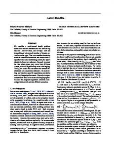
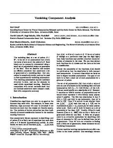
with p0/ , p1 ∈ R+ . This function is obviously a cascade of two L p -norms and is thus positively homogeneous of degree one. Figure 1(a) shows this function visualized as a tree. Naturally, any tree like the ones in Figure 1 corresponds to a function of the kind of Equation (1). In general, the n leaves of the tree correspond to the n coefficients of the vector x ∈ Rn and each inner node computes the L p -norm of its children using its specific p. We call the class of functions which is generated in this way L p -nested and the corresponding distributions, which are symmetric or invariant with respect to it, L p -nested symmetric distributions. L p -nested functions are much more flexible in creating different shapes of level sets than single L p -norms. Those level sets become the iso-density contours in the family of L p -nested symmetric distributions. Figure 2 shows a variety of contours generated by the simplest non-trivial L p -nested function shown in Equation (1). The shapes show the unit spheres for all possible combinations of p0/ , p1 ∈ {0.5, 1, 2, 10}. On the diagonal, p0/ and p1 are equal and therefore constitute L p -norms. The corresponding distributions are members of the L p -spherically symmetric class. To make general statements about general L p -nested functions, we introduce a notation that is suitable for the tree structure of L p -nested functions. As we will heavily use that notation in the remainder of the paper, we would like to emphasize the importance of the following paragraphs. We will illustrate the notation with an example below. Additionally, Figure 1 and Table 1 can be used for reference. We use multi-indices to denote the different nodes of the tree corresponding to an L p -nested function f . The function f = f0/ itself computes the value v0/ at the root node (see Figure 1). Those values are denoted by variables v. The functions corresponding to its children are denoted by f1 , ..., fℓ0/ , that is, f (·) = f0/ (·) = k( f1 (·), ..., fℓ0/ (·))k p0/ . We always use the letter “ℓ” indexed by the node’s multi-index to denote the total number of direct children of that node. The functions of 3412


(a) Equation (1) as tree.

(b) Equation (1) as tree in multi-index notation.

Figure 1: Equation (1) visualized as a tree with two different naming conventions. Figure (a) shows the tree where the nodes are labeled with the coefficients of x ∈ Rn . Figure (b) shows the same tree in multi-index notation where the multi-index of a node describes the path from the root node to that node in the tree. The leaves v1 , v2,1 and v2,2 still correspond to x1 , x2 and x3 , respectively, but have been renamed to the multi-index notation used in this article.

f (·) = f0/ (·)

L p -nested function

I = i1 , ..., im

Multi-index denoting a node in the tree: The single indices describe the path from the root node to the respective node I. All entries in x that correspond to the leaves in the subtree under

xI

the node I x Ib

All entries in x that are not leaves in the subtree under the node I

fI (·)

L p -nested function corresponding to the subtree under the node I

v0/

Function value at the root node

vI

Function value at an arbitrary node with multi-index I

ℓI

The number of direct children of a node I

nI v I,1:ℓI

The number of leaves in the subtree under the node I Vector with the function values at the direct children of a node I

Table 1: Summary of the notation used for L p -nested functions in this article. the children of the ith child of the root node are denoted by fi,1 , ..., fi,ℓi and so on. In this manner, an index is added for denoting the children of a particular node in the tree and each multi-index denotes the path to the respective node in the tree. For the sake of compact notation, we use upper case letters to denote a single multi-index I = i1 , ..., iℓ . The range of the single indices and the length of the multi-index should be clear from the context. A concatenation I, k of a multi-index I with a single index k corresponds to adding k to the index tuple, that is, I, k = i1 , ..., im , k. We use the 3413

S INZ AND B ETHGE

Figure 2: Variety of contours created by the L p -nested function of Equation (1) for all combinations of p0/ , p1 ∈ {0.5, 1, 2, 10}.

convention that I, 0/ = I. Those coefficients of the vector x that correspond to leaves of the subtree under a node with the index I are denoted by x I . The complement of those coefficients, that is, the ones that are not in the subtree under the node I, are denoted by x Ib. The number of leaves in a subtree under a node I is denoted by nI . If I denotes a leaf then nI = 1. The L p -nested function associated with the subtree under a node I is denoted by fI (xxI ) = ||( fI,1 (xxI,1 ), ..., fI,ℓI (xxI,ℓI ))⊤ || pI . 3414


Just like for the root node, we use the variable vI to denote the function value vI = fI (xxI ) of a subtree I. A vector with the function values of the children of I is denoted with bold font v I,1:ℓI where the colon indicates that we mean the vector of the function values of the ℓI children of node I: fI (xxI ) = ||( fI,1 (xxI,1 ), ..., fI,ℓI (xxI,ℓI ))⊤ || pI = ||(vI,1 , ..., vI,ℓI )⊤ || pI = ||vvI,1:ℓI || pI . Note that we can assign an arbitrary p to leaf nodes since ps for single variables always cancel. For that reason we can choose an arbitrary p for convenience and fix its value to p = 1. Figure 1(b) shows the multi-index notation for our example of Equation (1). To illustrate the notation: Let I = i1 , ..., id be the multi-index of a node in the tree. i1 , ..., id th describes the path to that node, that is, the respective node is the ith d child of the id−1 child of th the ith d−2 child of the ... of the i1 child of the root node. Assume that the leaves in the subtree below the node I cover the vector entries x2 , ..., x10 . Then x I = (x2 , ..., x10 ), x Ib = (x1 , x11 , x12 , ...), and nI = 9. Assume that node I has ℓI = 2 children. Those would be denoted by I, 1 and I, 2. The function realized by node I would be denoted by fI and only acts on x I . The value of the function would be fI (xxI ) = vI and the vector containing the values of the children of I would be v I,1:2 = (vI,1 , vI,2 )⊤ = ( fI,1 (xxI,1 ), fI,2 (xxI,2 ))⊤ . We now introduce a coordinate representation specially tailored to L p -nested symmetrically distributed variables: One of the most important consequences of the positive homogeneity of f is that it can be used to “normalize” vectors and, by that property, create a polar like coordinate representation of a vector x . Such polar-like coordinates generalize the coordinate representation for L p -norms by Gupta and Song (1997). Definition 1 (Polar-like Coordinates) We define the following polar-like coordinates for a vector x ∈ Rn : xi for i = 1, ..., n − 1, f (xx) r = f (xx).

ui =

The inverse coordinate transformation is given by xi = rui for i = 1, ..., n − 1, xn = r∆n un where ∆n = sgn xn and un =

|xn | f (xx) .

Note that un is not part of the coordinate representation since normalization with 1/ f (xx) decreases the degrees of freedom u by one, that is, un can always be computed from all other ui by solving f (uu) = f (xx/ f (xx)) = 1 for un . We use the term un only for notational simplicity. With a slight abuse of notation, we will use u to denote the normalized vector x / f (xx) or only its first n − 1 components. The exact meaning should always be clear from the context. The definition of the coordinates is exactly the same as the one by Gupta and Song (1997) with the only difference that the L p -norm is replaced by an L p -nested function. Just as in the case of L p -spherical coordinates, it will turn out that the determinant of the Jacobian of the coordinate 3415

S INZ AND B ETHGE

transformation does not depend on the value of ∆n and can be computed analytically. The determinant is essential for deriving the uniform distribution on the unit L p -nested sphere L f , that is, the 1-level set of f . Apart from that, it can be used to compute the radial distribution for a given L p -nested symmetric distribution. We start by stating the general form of the determinant in terms n of the partial derivatives ∂u ∂uk , uk and r. Afterwards we demonstrate that those partial derivatives have a special form and that most of them cancel in Laplace’s expansion of the determinant. Lemma 2 (Determinant of the Jacobian) Let r and u be defined as in Definition 1. The general ∂xi form of the determinant of the Jacobian J = ∂y j of the inverse coordinate transformation for ij

y1 = r and yi = ui−1 for i = 2, ..., n, is given by

! ∂un · uk + un . −∑ k=1 ∂uk n−1

| det J | = rn−1

(2)

Proof The proof can be found in the Appendix A. n The problematic parts in Equation (2) are the terms ∂u ∂uk , which obviously involve extensive usage of the chain rule. Fortunately, most of them cancel when inserting them back into Equation (2), leaving a comparably simple formula. The remaining part of this section is devoted to computing those terms and demonstrating how they vanish in the formula for the determinant. Before we state the general case we would like to demonstrate the basic mechanism through a simple example. We urge the reader to follow this example as it illustrates all important ideas about the coordinate transformation and its Jacobian.

Example 1 Consider an L p -nested function very similar to our introductory example of Equation (1): p1 p0/ f (xx) = (|x1 | p1 + |x2 | p1 ) p1 + |x3 | p0/ 0/ .

Setting u =

x f (xx)

and solving for u3 yields

p1

p1

f (uu) = 1 ⇔ u3 = 1 − (|u1 | + |u2 | )

p0/ p1

p1

0/

.

(3)

We would like to emphasize again, that u3 is actually not part of the coordinate representation and only used for notational simplicity. By construction, u3 is always positive. This is no restriction since Lemma 2 shows that the determinant of the Jacobian does not depend on its sign. However, when computing the volume and the surface area of the L p -nested unit sphere, it will become important since it introduces a factor of 2 to account for the fact that u3 (or un in general) can in principle also attain negative values. Now, consider G2 (uub2 ) = g2 (uub2 )

1−p0/

1−p0/ p/ p0/ p1 p1 p01 , = 1 − (|u1 | + |u2 | )

F1 (uu1 ) = f1 (uu1 ) p0/ −p1 = (|u1 | p1 + |u2 | p1 ) 3416

p0/ −p1 p1

,


where the subindices of u , f , g, G and F have to be read as multi-indices. The function gI computes the value of the node I from all other leaves that are not part of the subtree under I by fixing the value of the root node to one. G2 (uub2 ) and F1 (uu1 ) are terms that arise from applying the chain rule when computing the partial 3 derivatives ∂u ∂uk . Taking those partial derivatives can be thought of as peeling off layer by layer of Equation (3) via the chain rule. By doing so, we “move” on a path between u3 and uk . Each application of the chain rule corresponds to one step up or down in the tree. First, we move upwards in the tree, starting from u3 . This produces the G-terms. In this example, there is only one step upwards, but in general, there can be several, depending on the depth of un in the tree. Each step up will produce one G-term. At some point, we will move downwards in the tree to reach uk . This will produce the F-terms. While there are as many G-terms as upward steps, there is one term less when moving downwards. Therefore, in this example, there is one term G2 (uub2 ) which originates from using the chain rule upwards in the tree and one term F1 (uu1 ) from using it downwards. The indices correspond to the multi-indices of the respective nodes. Computing the derivative yields ∂u3 = −G2 (uub2 )F1 (uu1 )∆k |uk | p1 −1 . ∂uk By inserting the results in Equation (2) we obtain 2 1 G2 (uub2 )F1 (uu1 )|uk | p1 + u3 | J | = ∑ r2 k=1 2

= G2 (uub2 ) F1 (uu1 ) ∑ |uk | p1 + 1 − F1 (uu1 )F1 (uu1 )−1 (|u1 | p1 + |u2 | p1 ) k=1 2

2

k=1

k=1

= G2 (uub2 ) F1 (uu1 ) ∑ |uk | p1 + 1 − F1 (uu1 ) ∑ |uk | p1

!

p0/ p1

!

= G2 (uub2 ).

The example suggests that the terms from using the chain rule downwards in the tree cancel while the terms from using the chain rule upwards remain. The following proposition states that this is true in general. Proposition 3 (Determinant of the Jacobian) Let L be the set of multi-indices of the path from the leaf un to the root node (excluding the root node) and let the terms GI,ℓI (uuI,ℓ cI ) recursively be defined as pI,ℓ −pI uI,ℓ = GI,ℓI (uuI,ℓ cI ) = gI,ℓI (u cI ) I

ℓ−1

gI (uuIb) pI − ∑ fI, j (uuI, j ) pI j=1

! pI,ℓpI −pI I

where each of the functions gI,ℓI computes the value of the ℓth child of a node I as a function of its neighbors (I, 1), ..., (I, ℓI − 1) and its parent I while fixing the value of the root node to one. This is equivalent to computing the value of the node I from all coefficients u Ib that are not leaves in the subtree under I. Then, the determinant of the Jacobian for an L p -nested function is given by | det J | = rn−1 ∏ GL (uuLb ). L∈L

3417

S INZ AND B ETHGE

Proof The proof can be found in the Appendix A. Let us illustrate the determinant with two examples: Example 2 Consider a normal L p -norm n

∑ |xi | p

f (xx) =

i=1

! 1p

which is obviously also an L p -nested function. Resolving the equation for the last coordinate of 1 n−1 the normalized vector u yields gn (uunb) = un = 1 − ∑i=1 |ui | p p . Thus, the term Gn (uunb) is given by 1−p 1−p n−1 n−1 |ui | p p . This is exactly 1 − ∑i=1 |ui | p p which yields a determinant of | det J | = rn−1 1 − ∑i=1 the one derived by Gupta and Song (1997). Example 3 Consider the introductory example p0/ 1 p f (xx) = |x1 | p0/ + (|x2 | p1 + |x3 | p1 ) p1 0/ .

Normalizing and resolving for the last coordinate yields

p1 p1 u3 = (1 − |u1 | p0/ ) p0/ − |u2 | p1 1

2 ub2 )G2,2 (uu2,2 and the terms G2 (uub2 ) and G2,2 (uu2,2 c ) are given by c ) of the determinant | det J | = r G2 (u p1 −p0/

G2 (uub2 ) = (1 − |u1 | p0/ ) p0/ , 1 1−p p p1 p0/ p01/ p1 . G2,2 (uu2,2 c ) = (1 − |u1 | ) − |u2 |

Note the difference to Example 1 where x3 was at depth one in the tree while x3 is at depth two in the current case. For that reason, the determinant of the Jacobian in Example 1 involved only one G-term while it has two G-terms here.

3. L p -Nested Symmetric and L p -Nested Uniform Distribution In this section, we define the L p -nested symmetric and the L p -nested uniform distribution and derive their partition functions. In particular, we derive the surface area of an arbitrary L p -nested unit sphere L f = {xx ∈ Rn | f (xx) = 1} corresponding to an L p -nested function f . By Equation (5) of Fernandez et al. (1995) every ν-spherical and hence any L p -nested symmetric density has the form ρ(xx) =

φ( f (xx)) , f (xx)n−1 S f (1)

(4)

where S f is the surface area of L f and φ is a density on R+ . Thus, we need to compute the surface area of an arbitrary L p -nested unit sphere to obtain the partition function of Equation (4). 3418


Proposition 4 (Volume and Surface of the L p -nested Sphere) Let f be an L p -nested function and let I be the set of all multi-indices denoting the inner nodes of the tree structure associated with f . The volume V f (R) and the surface S f (R) of the L p -nested sphere with radius R are given by " #! Rn 2n 1 ℓI −1 ∑ki=1 nI,k nI,k+1 V f (R) = (5) ∏ B pI , pI n ∏ pℓI I −1 k=1 I∈I h i nI,k ℓI Γ n n ∏ k=1 pI R 2 h i, (6) = ℓI −1 nI n ∏ I∈I pI Γ pI #! " ℓI −1 k n n 1 ∑ I,k+1 I,k S f (R) = Rn−1 2n ∏ ℓI −1 ∏ B i=1 , (7) pI pI pI I∈I k=1 h i nI,k ℓI Γ ∏k=1 pI n−1 n h i (8) =R 2 ∏ ℓ −1 n I∈I pI I Γ I pI where B[a, b] =

Γ[a]Γ[b] Γ[a+b]

denotes the β-function.

Proof The proof can be found in the Appendix B. Inserting the surface area in Equation 4, we obtain the general form of an L p -nested symmetric distribution for any given radial density φ. Corollary 5 (L p -nested Symmetric Distribution) Let f be an L p -nested function and φ a density on R+ . The corresponding L p -nested symmetric distribution is given by ρ(xx) = =

φ( f (xx)) f (xx)n−1 S f (1)



φ( f (xx))  pℓI I −1 ∏ B 2n f (xx)n−1 ∏ I∈I k=1 ℓI −1

"

∑ki=1 nI,k pI

#−1  nI,k+1 . , pI

(9)

The results of Fernandez et al. (1995) imply that for any ν-spherically symmetric distribution, the radial part is independent of the directional part, that is, r is independent of u . The distribution of u is entirely determined by the choice of ν, or by the L p -nested function f in our case. The distribution of r is determined by the radial density φ. Together, an L p -nested symmetric distribution is determined by both, the L p -nested function f and the choice of φ. From Equation (9), we can see that its density function must be the inverse of the surface area of L f times the radial density when transforming (4) into the coordinates of Definition 1 and separating r and u (the factor f (xx)n−1 = r cancels due to the determinant of the Jacobian). For that reason we call the distribution of u uniform on the L p -sphere L f in analogy to Song and Gupta (1997). Next, we state its form in terms of the coordinates u. Proposition 6 (L p -nested Uniform Distribution) Let f be an L p -nested function. Let L be the set of multi-indices on the path from the root node to the leaf corresponding to xn . The uniform 3419

S INZ AND B ETHGE

distribution on the L p -nested unit sphere, that is, the set L f = {xx ∈ Rn | f (xx) = 1} is given by the following density over u1 , ..., un−1  #−1  " ℓ −1 k I ∏L∈L GL (uuLb ) .  pℓI I −1 ∏ B ∑i=1 nI,k , nI,k+1 ρ(u1 , , ..., un−1 ) = ∏ n−1 2 p p I I I∈I k=1 Proof Since the L p -nested sphere is a measurable and compact set, the density of the uniform distribution is simply one over the surface area of the L p -nested unit sphere. The surface S f (1) is given by Proposition 4. Transforming S f 1(1) into the coordinates of Definition 1 introduces the determinant of the Jacobian from Proposition 3 and an additional factor of 2 since the (u1 , ..., un−1 ) ∈ Rn−1 have to account for both half-shells of the L p -nested unit sphere, that is, to account for the fact that un could have been be positive or negative. This yields the expression above.

Example 4 Let us again demonstrate the proposition at the special case where f is an L p -norm 1 f (xx) = ||xx|| p = (∑ni=1 |xi | p ) p . Using Proposition 4, the surface area is given by n

S||·|| p = 2

1

ℓ0/ −1

pℓ0/0/ −1

k=1

∏B

∑ki=1 nk p0/

2n Γn

h i 1

p nk+1 h i. , = p0/ pn−1 Γ np

1−p n−1 The factor Gn (uunb) is given by 1 − ∑i=1 |ui | p p (see the L p -norm example before), which, after including the factor 2, yields the uniform distribution on the L p -sphere as defined in Song and Gupta (1997) h i ! 1−p p n−1 pn−1 Γ np p i h u 1 − ∑ |ui | . p(u ) = i=1 2n−1 Γn 1p Example 5 As a second illustrative example, we consider the uniform density on the L p -nested unit ball, that is, the set {xx ∈ Rn | f (xx) ≤ 1}, and derive its radial distribution φ. The density of the uniform distribution on the unit L p -nested ball does not depend on x and is given by ρ(xx) = 1/V f (1). Transforming the density into the polar-like coordinates with the determinant from Proposition 3 yields  " #−1  n−1 ℓ −1 k I nr ∏L∈L GL (uuLb ) 1  pℓI I −1 ∏ B ∑i=1 nI,k , nI,k+1 . = ∏ n−1 2 pI pI V f (1) I∈I k=1 After separating out the uniform distribution on the L p -nested unit sphere, we obtain the radial distribution φ(r) = nrn−1 for 0 < r ≤ 1 which is a β-distribution with parameters n and 1. 3420


The radial distribution from the preceeding example is of great importance for our sampling scheme derived in Section 6. The idea behind it is the following: First, a sample from a “simple” L p -nested symmetric distribution is drawn. Since the radial and the uniform component on the L p nested unit sphere are statistically independent, we can get a sample from the uniform distribution on the L p -nested unit sphere by simply normalizing the sample from the simple distribution. Afterwards we can multiply it with a radius drawn from the radial distribution of the L p -nested symmetric distribution that we actually want to sample from. The role of the simple distribution will be played by the uniform distribution within the L p -nested unit ball. Sampling from it is basically done by applying the steps in Proposition 4’s proof backwards. We lay out the sampling scheme in more detail in Section 6.

4. Marginals In this section we discuss two types of marginals: First, we demonstrate that, in contrast to L p spherically symmetric distributions, marginals of L p -nested symmetric distributions are not necessarily L p -nested symmetric again. The second type of marginals we discuss are obtained by collapsing all leaves of a subtree into the value of the subtree’s root node. For that case we derive an analytical expression and show that the values of the root node’s children follow a special kind of Dirichlet distribution. Gupta and Song (1997) show that marginals of L p -spherically symmetric distributions are again L p -spherically symmetric. This does not hold, however, for L p -nested symmetric distributions. This can be shown by a simple counterexample. Consider the L p -nested function p1 p0/ f (xx) = (|x1 | p1 + |x2 | p1 ) p1 + |x3 | p0/ 0/ .

The uniform distribution inside the L p -nested ball corresponding to f is given by h i h i np1 p0/ Γ p21 Γ p30/ h i h i h i. ρ(xx) = 23 Γ2 p11 Γ p20 Γ p10 The marginal ρ(x1 , x3 ) is given by

h i h i p1 np1 p0/ Γ p21 Γ p30/ p1 h i h i h i (1 − |x3 | p0/ ) p0/ − |x1 | p1 1 . ρ(x1 , x3 ) = 23 Γ2 p11 Γ p20 Γ p10

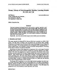
This marginal is not L p -spherically symmetric. Since any L p -nested symmetric distribution in two dimensions must be L p -spherically symmetric, it cannot be L p -nested symmetric as well. Figure 3 shows a scatter plot of the marginal distribution. Besides the fact that the marginals are not contained in the family of L p -nested symmetric distributions, it is also hard to derive a general form for them. This is not surprising given that the general form of marginals for L p -spherically symmetric distributions involves an integral that cannot be solved analytically in general and is therefore not very useful in practice (Gupta and Song, 1997). For that reason we cannot expect marginals of L p -nested symmetric distributions to have a simple form. In contrast to single marginals, it is possible to specify the joint distribution of leaves and inner nodes of an L p -nested tree if all descendants of their inner nodes in question have been integrated 3421

S INZ AND B ETHGE

a

b

c

d

Figure 3: Marginals of L p -nested symmetric distributions are not necessarily L p -nested symmetric: Figure (a) shows a scatter plot of the (x1 , x2 )-marginal of the counterexample in the text with p0/ = 2 and p1 = 12 . Figure (d) displays the corresponding L p -nested sphere. (bc) show the univariate marginals for the scatter plot. Since any two-dimensional L p nested symmetric distribution must be L p -spherically symmetric, the marginals should be identical. This is clearly not the case. Thus, (a) is not L p -nested symmetric.

out. For the simple function above (the same that has been used in Example 1), the joint distribution of x3 and v1 = k(x1 , x2 )⊤ k p1 would be an example of such a marginal. Since marginalization affects 3422


the L p -nested tree vertically, we call this type of marginals layer marginals. In the following, we present their general form. From the form of a general L p -nested function and the corresponding symmetric distribution, one might think that the layer marginals are L p -nested symmetric again. However, this is not the case since the distribution over the L p -nested unit sphere would deviate from the uniform distribution in most cases if the distribution of its children were L p -spherically symmetric. Proposition 7 Let f be an L p -nested function. Suppose we integrate out complete subtrees from the tree associated with f , that is, we transform subtrees into radial times uniform variables and integrate out the latter. Let J be the set of multi-indices of those nodes that have become new leaves, that is, whose subtrees have been removed, and let nJ be the number of leaves (in the original tree) in the subtree under the node J. Let x Jb ∈ Rm denote those coefficients of x that are still part of that smaller tree and let v J denote the vector of inner nodes that became new leaves. The joint distribution of x Jb and v J is given by ρ(xxJb , v J ) =

φ( f (xxJb , v J ))

∏ S f ( f (xxJb , v J )) J∈ J

vJnJ −1 .

(10)

Proof The proof can be found in the Appendix C.

Equation (10) has an interesting special case when considering the joint distribution of the root node’s children. Corollary 8 The children of the root node v 1:ℓ0/ = (v1 , ..., vℓ0/ )⊤ follow the distribution

ρ(vv1:ℓ0/ ) =

pℓ0/0/ −1 Γ

h i n p0/

0/ f (v1 , ..., vℓ0/ )n−1 2m ∏ℓk=1 Γ

ℓ0/

h i φ ( f (v1 , ..., vℓ0/ )) ∏ vini −1 nk p0/

i=1

where m ≤ ℓ0/ is the number of leaves directly attached to the root node. In particular, v 1:ℓ0/ can be written as the product RU, where R is theh L p -nestedi radius and the single |Ui | p0/ are Dirichlet

distributed, that is, (|U1 | p0/ , ..., |Uℓ0/ | p0/ ) ∼ Dir

nℓ0/ n1 p0/ , ..., p0/

.

Proof The joint distribution is simply the application of Proposition (7). Note that f (v1 , ..., vℓ0/ ) = ||vv1:ℓ0/ || p0/ . Applying the pointwise transformation si = |ui | p0/ yields n1 nℓ0/ p0/ p0/ (|U1 | , ..., |Uℓ0/ −1 | ) ∼ Dir , ..., . p0/ p0/

The Corollary shows that the values fI (xxI ) at inner nodes I, in particular the ones directly below the root node, deviate considerably from L p -spherical symmetry. If they were L p -spherically symmetric, the |Ui | p should follow a Dirichlet distribution with parameters αi = 1p as has been already shown by Song and Gupta (1997). The Corollary is a generalization of their result. We can use the Corollary to prove an interesting fact about L p -nested symmetric distributions: The only factorial L p -nested symmetric distribution must be L p -spherically symmetric. 3423

S INZ AND B ETHGE

Proposition 9 Let x be L p -nested symmetric distributed with independent marginals. Then x is L p -spherically symmetric distributed. In particular, x follows a p-generalized Normal distribution. Proof The proof can be found in the Appendix D. One immediate implication of Proposition 9 is that there is no factorial probability model correq sponding to mixed norm regularizers which have the form ∑ki=1 kxxIk k p where the index sets Ik form a partition of the dimensions 1, ..., n (see, e.g., Zhao et al., 2008; Yuan and Lin, 2006; Kowalski et al., 2008). Many machine learning algorithms are equivalent to minimizing the sum of a reguw) and a loss function L(w w, x 1 , ..., x m ) over the coefficient vector w . If the exp (−R(w w)) larizer R(w w, x 1 , ..., x m )) correspond to normalizeable density models, the minimizing solution and exp (−L(w of the objective function can be seen as the maximum a posteriori (MAP) estimate of the postew|xx1 , ..., xm ) ∝ p(w w) · p(xx1 , ..., xm |w w) = exp (−R(w w)) · exp (−L(w w, x1 , ..., xm )). In that sense, rior p (w the regularizer naturally corresponds to the prior and the loss function corresponds to the likelihood. Very often, regularizers are specified as a norm over the coefficient vector w which in turn correspond to certain priors. For example, in Ridge regression (Hoerl, 1962) the coefficients are wk22 which corresponds to a factorial zero mean Gaussian prior on w . The L1 -norm regularized via kw wk1 in the LASSO estimator (Tibshirani, 1996), again, is equivalent to a factorial Laplacian prior kw on w . Like in these two examples, regularizers often correspond to a factorial prior. Mixed norm regularizers naturally correspond to L p -nested symmetric distributions. Proposition 9 shows that there is no factorial prior that corresponds to such a regularizer. In particular, it implies that the prior cannot be factorial between groups and coefficients at the same time. This means that those regularizers implicitly assume statistical dependencies between the coefficient variables. Interestingly, for q = 1 and p = 2 the intuition behind these regularizers is exactly that whole groups Ik get switched on at once, but the groups are sparse. The Proposition shows that this might not only be due to sparseness but also due to statistical dependencies between the coefficients within one group. The L p -nested symmetric distribution which implements independence between groups will be further discussed below as a generalization of the p-generalized Normal (see Section 8). Note that the marginals can be independent if the regularizer is of the form ∑ki=1 kxxIk k pp . However, in this case p = q and the L p -nested function collapses to a simple L p -norm which means that the regularizer is not mixed norm.

5. Maximum Likelihood Estimation of L p -Nested Symmetric Distributions In this section, we describe procedures for maximum likelihood fitting of L p -nested symmetric distributions on data. We provide a toolbox online for fitting L p -spherically symmetric and L p -nested symmetric distributions to data. The toolbox can be downloaded at http://www.kyb.tuebingen. mpg.de/bethge/code/. Depending on which parameters are to be estimated, the complexity of fitting an L p -nested symmetric distribution varies. We start with the simplest case and later continue with more complex ones. Throughout this subsection, we assume that the model has the form p(xx) = ρ(W x ) · | detW | = φ(W x) · | detW | where W ∈ Rn×n is a complete whitening matrix. This means that given any f (W x )n−1 S f (1) whitening matrix W0 , the freedom in fitting W is to estimate an orthonormal matrix Q ∈ SO(n) such that W = QW0 . This is analogous to the case of elliptically contoured distributions where the 3424


distributions can be endowed with 2nd-order correlations via W . In the following, we ignore the determinant of W since data points can always be rescaled such that detW = 1. The simplest case is to fit the parameters of the radial distribution when the tree structure, the values of the pI , and W are fixed. Due to the special form of L p -nested symmetric distributions (4), it then suffices to carry out maximum likelihood estimation on the radial component only, which renders maximum likelihood estimation efficient and robust. This is because the only remaining parameters are the parameters ϑ of the radial distribution and, therefore, ϑ) = argmaxϑ (− log S f ( f (W x )) + log φ( f (W x )|ϑ ϑ)) argmaxϑ log ρ(W x |ϑ ϑ). = argmaxϑ log φ( f (W x )|ϑ In a slightly more complex case, when only the tree structure and W are fixed, the values of the pI , I ∈ I and ϑ can be jointly estimated via gradient ascent on the log-likelihood. The gradient for a single data point x with respect to the vector p that holds all pI for all I ∈ I is given by ∇ p log ρ(W x ) =

d (n − 1) log φ( f (W x )) · ∇ p f (W x ) − ∇ p f (W x ) − ∇ p log S f (1). dr f (W x )

For i.i.d. data points xi the joint gradient is given by the sum over the gradients for the single data points. Each of them involves the gradient of f as well as the gradient of the log-surface area of L f with respect to p , which can be computed via the recursive equations   if I is not a prefix of J  0 ∂ 1−pI pI −1 ∂ if I is a prefix of J vI = vI vI,k · ∂pJ vI,k  ∂pJ  p −p ℓ v J J J J  if J = I v ∑ v · log vJ,k − log vJ pJ

J

k=1 J,k

and

" # n ∂ ℓJ − 1 ℓJ −1 ∑k+1 ∑k+1 J,k i=1 i=1 nJ,k log S f (1) = − + ∑Ψ ∂pJ pJ pJ p2J k=1 " # ℓJ −1 nJ,k+1 nJ,k+1 ∑ki=1 nJ,k ∑ki=1 nJ,k ℓJ −1 − ∑Ψ − ∑Ψ , pJ pJ p2J p2J k=1 k=1 where Ψ[t] = dtd log Γ[t] denotes the digamma function. When performing the gradient ascent, one needs to set 0 as a lower bound for p . Note that, in general, this optimization might be a highly non-convex problem. On the next level of complexity, only the tree structure is fixed, and W can be estimated along with the other parameters by joint optimization of the log-likelihood with respect to p, ϑ and W . Certainly, this optimization problem is also not convex in general. Usually, it is numerically more robust to whiten the data first with some whitening matrix W0 and perform a gradient ascent on the special orthogonal group SO(n) with respect to Q for optimizing W = QW0 . Given the gradient ∇W log ρ(W x ) of the log-likelihood, the optimization can be carried out by performing line searches along geodesics as proposed by Edelman et al. (1999) (see also Absil et al. (2007)) or by projecting ∇W log ρ(W x ) on the tangent space TW SO(n)) and performing a line search along SO(n) in that direction as proposed by Manton (2002). 3425

S INZ AND B ETHGE

The general form of the gradient to be used in such an optimization scheme can be defined as ∇W log ρ(W x ) =∇W (−(n − 1) · log f (W x ) + log φ( f (W x ))) (n − 1) d log φ(r) =− · ∇y f (W x ) · x ⊤ + ( f (W x )) · ∇y f (W x ) · x ⊤ , f (W x ) dr where the derivatives of f with respect to y are defined by recursive equations   0 ∂ vI = sgn yi  ∂yi  1−pI pI −1 ∂ vI · vI,k · ∂yi vI,k

if i 6∈ I if vI,k = |yi | for i ∈ I, k.

Note, that f might not be differentiable at y = 0. However, we can always define a sub-derivative at zero, which is zero for pI 6= 1 and [−1, 1] for pI = 1. Again, the gradient for i.i.d. data points x i is given by the sum over the single gradients. Finally, the question arises whether it is possible to estimate the tree structure from data as well. A simple heuristic would be to start with a very large tree, for example, a full binary tree, and to prune out inner nodes for which the parents and the children have sufficiently similar values for their pI . The intuition behind this is that if they were exactly equal, they would cancel in the L p -nested function. This heuristic is certainly sub-optimal. Firstly, the optimization will be time consuming since there can be about as many pI as there are leaves in the L p -nested tree (a full binary tree on n dimensions will have n − 1 inner nodes) and due to the repeated optimization after the pruning steps. Secondly, the heuristic does not cover all possible trees on n leaves. For example, if two leaves are separated by the root node in the original full binary tree, there is no way to prune out inner nodes such that the path between those two nodes will not contain the root node anymore. The computational complexity for the estimation of all other parameters despite the tree structure is difficult to assess in general because they depend, for example, on the particular radial distribution used. While the maximum likelihood estimation of a simple log-Normal distribution only involves the computation of a mean and a variance which are in O (m) for m data points, a mixture of log-Normal distributions already requires an EM algorithm which is computationally more expensive. Additionally, the time it takes to optimize the likelihood depends on the starting point as well as the convergence rate, and we neither have results about the convergence rate nor is it possible to make problem independent statements about a good initialization of the parameters. For this reason we state only the computational complexity of single steps involved in the optimization. Computation of the gradient ∇ p log ρ(W x ) involves the derivative of the radial distribution, the computation of the gradients ∇ p f (W x ) and ∇ p S f (1). Assuming that the derivative of the radial distribution can be computed in O (1) for each single data point, the costly steps are the other two gradients. Computing ∇ p f (W x ) basically involves visiting each node of the tree once and performing a constant number of operations for the local derivatives. Since every inner node in an L p -nested tree must have at least two children, the worst case would be a full binary tree which has 2n − 1 nodes and leaves. Therefore, the gradient can be computed in O (nm) for m data points. For similar reasons, f (W x ), ∇ p log S f (1), and the evaluation of the likelihood can also be computed in O (nm). This means that each step in the optimization of p can be done O (nm) plus the computational costs for the line search in the gradient ascent. When optimizing for W = QW0 as well, the computational 3426


costs per step increase to O (n3 + n2 m) since m data points have to be multiplied with W at each iteration (requiring O (n2 m) steps), and the line search involves projecting Q back onto SO(n) which requires an inverse matrix square root or a similar computation in O (n3 ). For comparison, each step of fast ICA (Hyvärinen and O., 1997) for a complete demixing matrix takes O (n2 m) when using hierarchical orthogonalization and O (n2 m + n3 ) for symmetric orthogonalization. The same applies to fitting an ISA model (Hyvärinen and Hoyer, 2000; Hyvärinen and Köster, 2006, 2007). A Gaussian Scale Mixture (GSM) model does not need to estimate another orthogonal rotation Q because it belongs to the class of spherically symmetric distributions and is, therefore, invariant under transformations from SO(n) (Wainwright and Simoncelli, 2000). Therefore, fitting a GSM corresponds to estimating the parameters of the scale distribution which is O (nm) in the best case but might be costlier depending on the choice of the scale distribution.

6. Sampling from L p -Nested Symmetric Distributions In this section, we derive a sampling scheme for arbitrary L p -nested symmetric distributions which can for example be used for solving integrals when using L p -nested symmetric distributions for Bayesian learning. Exact sampling from an arbitrary L p -nested symmetric distribution is in fact straightforward due to the following observation: Since the radial and the uniform component are independent, normalizing a sample from any L p -nested symmetric distribution to f -length one yields samples from the uniform distribution on the L p -nested unit sphere. By multiplying those uniform samples with new samples from another radial distribution, one obtains samples from another L p -nested symmetric distribution. Therefore, for each L p -nested function f , a single L p -nested symmetric distribution which can be easily sampled from is enough. Sampling from all other L p -nested symmetric distributions with respect to f is then straightforward due to the method we just described. Gupta and Song (1997) sample from the p-generalized Normal distribution since it has independent marginals which makes sampling straightforward. Due to Proposition 9, no such factorial L p -nested symmetric distribution exists. Therefore, a sampling scheme like that for L p -spherically symmetric distributions is not applicable. Instead we choose to sample from the uniform distribution inside the L p -nested unit ball for which we already computed the radial distribution in Example 5. The distribution has the form ρ(xx) = V 1(1) . In order to sample from that distribution, we will first f only consider the uniform distribution in the positive quadrant of the unit L p -nested ball which has n the form ρ(xx) = V 2(1) . Samples from the uniform distributions inside the whole ball can be obtained f by multiplying each coordinate of a sample with independent samples from the uniform distribution over {−1, 1}. The idea of the sampling scheme for the uniform distribution inside the L p -nested unit ball is based on the computation of the volume of the L p -nested unit ball in Proposition 4. The basic mechanism underlying the sampling scheme below is to apply the steps of the proof backwards, which is based on the following idea: The volume of the L p -unit ball can be computed by computing its volume on the positive quadrant only and multiplying the result with 2n afterwards. The key is now to not transform the whole integral into radial and uniform coordinates at once, but successively upwards in the tree. We will demonstrate this through a brief example which also should make the sampling scheme below more intuitive. Consider the L p -nested function p0/ 1 p f (xx) = |x1 | p0/ + (|x2 | p1 + |x3 | p1 ) p1 0/ . 3427

S INZ AND B ETHGE

To solve the integral

Z

{xx: f (xx)≤1 & x ∈Rn+ }

dxx,

we first transform x2 and x3 into radial and uniform coordinates only. According to Proposition 3 the determinant of the mapping (x2 , x3 ) 7→ (v1 , u) ˜ = (kxx2:3 k p1 , x 2:3 /kxx2:3 k p1 ) is given by v1 (1− u˜ p1 ) Therefore the integral transforms into Z

{xx: f (xx)≤1 & x∈Rn+ }

dxx =

Z

{v1 ,x1 : f (x1 ,v1 )≤1 & x1 ,v1 ∈R+ }

Z Z

v1 (1 − u˜ p1 )

1−p1 p1

1−p1 p1

.

dx1 dv1 d u. ˜

Now we can separate the integrals over x1 and v1 , and the integral over u, ˜ since the boundary of the outer integral does only depend on v1 and not on u: ˜ Z

{xx: f (xx)≤1 & x ∈Rn+ }

dxx =

Z

p1

(1 − u˜ )

1−p1 p1

d u˜ ·

Z

{v1 ,x1 : f (x1 ,v1 )≤1 & x1 ,v1 ∈R+ }

Z

v1 dx1 dv1 .

The value of the first integral is known explicitly since the integrand equals the uniform distribution on the k · k p1 -unit sphere. Therefore, the value of the integral must be its normalization constant which we can get using Proposition 4: h i2 Z Γ p11 · p1 1−p1 h i . (1 − u˜ p1 ) p1 d u˜ = Γ p21

An alternative way to arrive at this result is to use the transformation s = u˜ p1 and to notice that the integrand is a Dirichlet distribution with parameters αi = p11 . The normalization constant of the Dirichlet distribution and the constants from the determinant of the Jacobian of the transformation yield the same result. To compute the remaining integral, the same method can be applied again yielding the volume of the L p -nested unit ball. The important part for the sampling scheme, however, is not the volume itself but the fact that the intermediate results in this integration process equal certain distributions. As shown in Example 5 the radial distribution of the uniform distribution on the unit ball is β [n, 1], and as just indicated by the example above, the intermediate results can be seen as transformed variables from a Dirichlet distribution. This fact holds true even for more complex L p -nested unit balls although the parameters of the Dirichlet distribution can be slightly different. Reversing the steps leads us to the following sampling scheme. First, we sample from the β-distribution which gives us the radius v0/ on the root node. Then we sample from the appropriate Dirichlet distribution and exponentiate the samples by p10/ which transforms them into the analogs of the variable u from above. Scaling the result with the sample v0/ yields the values of the root node’s children, that is, the analogs of x1 and v1 . Those are the new radii for the levels below them where we simply repeat this procedure with the appropriate Dirichlet distributions and exponents. The single steps are summarized in Algorithm 1. The computational complexity of the sampling scheme is O (n). Since the sampling procedure is like expanding the tree node by node starting with the root, the number of inner nodes and leaves is the total number of samples that have to be drawn from Dirichlet distributions. Every node in an L p -nested tree must at least have two children. Therefore, the maximal number of inner nodes and leaves is 2n − 1 for a full binary tree. Since sampling from a Dirichlet distribution is also in O (n), the total computational complexity for one sample is in O (n). 3428


Algorithm 1 Exact sampling algorithm for L p -nested symmetric distributions Input: The radial distribution φ of an L p -nested symmetric distribution ρ for the L p -nested function f. Output: Sample x from ρ. Algorithm 1. Sample v0/ from a beta distribution β [n, 1]. 2. For each inner node I of the with f , sample the auxiliary variable s I from h tree associated i nI,ℓI nI,1 a Dirichlet distribution Dir pI , ..., pI where nI,k are the number of leaves in the subtree under node I, k. Obtain coordinates on the L p -nested sphere within the positive orthant by 1

p s I 7→ s I I = u˜ I (the exponentiation is taken component-wise).

3. Transform these samples to Cartesian coordinates by vI · u˜ I = v I,1:ℓI for each inner node, starting from the root node and descending to lower layers. The components of v I,1:ℓI constitute / the radius had been sampled in step 1. the radii for the layer direct below them. If I = 0, 4. Once the two previous steps have been repeated until no inner node is left, we have a sample x from the uniform distribution in the positive quadrant. Normalize x to get a uniform sample x from the sphere u = f (x x) . 5. Sample a new radius v˜0/ from the radial distribution of the target radial distribution φ and obtain the sample via x˜ = v˜0/ · u . 6. Multiply each entry xi of x˜ by an independent sample zi from the uniform distribution over {−1, 1}.

7. Robust Bayesian Inference of the Location For L p -spherically symmetric distributions with a location and a scale parameter p(xx|µµ, τ) = τn ρ(kτ(xx − µ )k p ), Osiewalski and Steel (1993) derived the posterior in closed form using a prior p(µµ, τ) = p(µ) · c · τ−1 , and showed that p(xx, µ ) does not depend on the radial distribution φ, that is, the particular type of L p -spherically symmetric distributions used for a fixed p. The prior on τ corresponds to an improper Jeffrey’s prior which is used to represent lack of prior knowledge on the scale. The main implication of their result is that Bayesian inference of the location µ under that prior on the scale does not depend on the particular type of L p -spherically symmetric distribution used for inference. This means that under the assumption of an L p -spherically symmetric distributed variable, for a fixed p, one has to know the exact form of the distribution in order to compute the location parameter. It is straightforward to generalize their result to L p -nested symmetric distributions and, hence, making it applicable to a larger class of distributions. Note that when using any L p -nested symmetric distribution, introducing a scale and a location via the transformation x 7→ τ(xx − µ ) introduces a factor of τn in front of the distribution. 3429

S INZ AND B ETHGE

Proposition 10 For fixed values p0/ , p1 , ... and two independent priors p(µµ, τ) = p(µµ) · cτ−1 of the location µ and the scale τ where the prior on τ is an improper Jeffrey’s prior, the joint distribution p(xx, µ ) is given by p(xx, µ ) = f (xx − µ )−n · c ·

1 · p(µµ), Z

where Z denotes the normalization constant of the L p -nested uniform distribution. Proof Given any L p -nested symmetric distribution ρ( f (xx)), the transformation into the polar-like coordinates yields the following relation 1=

Z

ρ( f (xx))dxx =

Z Z

∏ GL (uuLb )rn−1 ρ(r)drduu =

L∈L

Z

∏ GL (uuLb )duu ·

L∈L

Z

rn−1 ρ(r)dr.

Since ∏L∈L GL (uuLb ) is the unnormalized uniform distribution on the L p -nested unit sphere, the integral must equal the normalization constant which we denote with Z for brevity (see Proposition 6 for an explicit expression). This implies that ρ has to fulfill 1 = Z

Z

rn−1 ρ(r)dr.

Writing down the joint distribution of x , µ and τ, and using the substitution s = τ f (xx − µ ) we obtain p(xx, µ ) = =

Z

Z

τn ρ( f (τ(xx − µ ))) · cτ−1 · p(µµ)dτ sn−1 ρ(s) · c · p(µµ) f (xx − µ )−n ds

= f (xx − µ )−n · c ·

1 · p(µµ). Z

Note that this result could easily be extended to ν-spherical distributions. However, in this case the normalization constant Z cannot be computed for most cases and, therefore, the posterior would not be known explicitly.

8. Relations to ICA, ISA and Over-Complete Linear Models In this section, we explain the relations among L p -spherically symmetric, L p -nested symmetric, ICA and ISA models. For a general overview see Figure 4. The density model underlying ICA models the joint distribution of the signal x as a linear superposition of statistically independent hidden sources Ayy = x or y = W x . If the marginals of the hidden sources belong to the exponential power family, we obtain the p-generalized Normal which is a subset of the L p -spherically symmetric class. The p-generalized Normal distribution p(yy) ∝ exp(−τkyyk pp ) is a density model that is often used in ICA algorithms for kurtotic natural signals like images and sound by optimizing a demixing matrix W w.r.t. to the model p(yy) ∝ exp(−τkW x k pp ) (Lee and Lewicki, 2000; Zhang et al., 2004; Lewicki, 2002). It can be 3430


Lp-nested symmetric

ISA

Lp-nested ISA Lp-spherically symmetric

ICA

p-generalized Normal

L2-spherically symmetric

Gaussian

Figure 4: Relations between the different classes of distributions: Arrows indicate that the child class is a specialization (subset) of the parent class. Polygon-shaped classes are intersections of those parent classes which are connected via edges with round arrow-heads. For one-dimensional subspaces ISA is a superclass of ICA. All classes belonging to ISA are colored white or light gray. L p -nested symmetric distributions are a superclass of L p spherically symmetric distributions. All L p -nested symmetric models are colored dark or light gray. L p -nested ISA models live in the intersection of L p -nested symmetric distributions and ISA models. Those L p -nested ISA models that are L p -spherically symmetric are also ICA models: This is the class of p-generalized Normal distributions. If p is fixed to two, one obtains the L2 -spherically symmetric distributions. The only class of distributions in the intersection between spherically symmetric distributions and ICA models is the Gaussian.

shown that the p-generalized Normal is the only factorial model in the class of L p -spherically symmetric models (Sinz et al., 2009a), and, by Proposition 9, also the only factorial L p -nested symmetric distribution. An important generalization of ICA is the independent subspace analysis (ISA) proposed by Hyvärinen and Hoyer (2000) and by Hyvärinen and Köster (2007) who used L p -spherically symmetric distributions to model the single subspaces, that is, each ρk below was L p -spherically symmetric. Like in ICA, ISA models the hidden sources of the signal as a product of multivariate distributions: K

ρ(yy) = ∏ ρk (yyIk ). k=1

Here, y = W x and Ik are index sets selecting the different subspaces from the responses of W to x . The collection of index sets Ik forms a partition of 1, ..., n. ICA is a special case of ISA in which 3431

S INZ AND B ETHGE

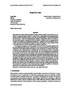
Ik = {k} such that all subspaces are one-dimensional. For the ISA models used by Hyvärinen et al. the distribution on the subspaces was chosen to be either spherically or L p -spherically symmetric. In its general form, ISA is not a generalization of L p -spherically symmetric distributions. The most general ISA model for the transformed data y = W x does not assume a certain type of distribution on the single subspace like in Hyvärinen and Köster (2007). While one could say for any non-factorial distribution that a factorial product over subspaces is a generalization, this is certainly a trivial step. Only in this particular sense is the particular ISA model by Hyvärinen and Köster (2007) a generalization of L p -spherically symmetric distributions. In contrast to ISA, L p -nested symmetric distributions generally do not make an independence assumption on the “subspaces”. In fact, for most of the models the subspaces will be dependent (see also our diagram in Figure 4). Therefore, not every ISA model is automatically L p -nested symmetric and vice versa. In fact, in Sinz et al. (2009b) we have demonstrated for natural images that the dependencies between subspaces is stronger than the dependencies within subspaces on natural image patches. This is in stark contrast to the assumptions underlying ISA. Note also that the product of L p -spherically symmetric distributions used by Hyvärinen and Köster (2007) is not an L p -nested function (Equation (6) in Hyvärinen and Köster, 2007) since the single a j can be different and, therefore, the overall function is not positively homogeneous in general. ICA and ISA have been used to infer features from natural signals, in particular from natural images. However, as mentioned by several authors (Zetzsche et al., 1993; Simoncelli, 1997; Wainwright and Simoncelli, 2000) and demonstrated quantitatively by Bethge (2006) and Eichhorn et al. (2009), the assumptions underlying linear ICA are not well matched by the statistics of the pixel intensities of natural images. A reliable parametric way to assess how well the independence assumption is met by a signal at hand is to fit a more general class of distributions that contains factorial as well as non-factorial distributions which both can equally well reproduce the marginals. By comparing the likelihood on held out test data between the best fitting non-factorial and the best-fitting factorial case, one can assess how well the sources can be described by a factorial distribution. For natural images, for example, one can use an arbitrary L p -spherically symmetric distribution ρ(kW x k p ), fit it to the whitened data and compare its likelihood on held out test data to the one of the p-generalized Normal distribution (Sinz and Bethge, 2009). Since any choice of radial distribution φ determines a particular L p -spherically symmetric distribution, the idea is to explore the space between factorial and non-factorial models by using a very flexible density φ on the radius. Note that having an explicit expression of the normalization constant allows for particularly reliable model comparisons via the likelihood. For many graphical models, for instance, such an explicit and computable expression is often not available. The same type of dependency-analysis can be carried out for ISA using L p -nested symmetric distributions (Sinz et al., 2009b). Figure 5 shows the L p -nested tree corresponding to an ISA with four subspaces. In general, for such trees, each inner node—except the root node—corresponds to a single subspace. When using the radial distribution p0/ p0/ v0n−1 v /i h φ0/ (v0/ ) = − 0/ , n exp n s Γ p0/ s p0/ 3432

(11)


Figure 5: Tree corresponding to an L p -nested ISA model. the subspaces v1 , ..., vℓ0/ become independent and one obtains an ISA model of the form 1 f (yy) p0/ y ρ(y ) = exp − Z s ! ℓ0/ kyyIk k pk ∑k=1 1 = exp − Z s h i ! ℓk −1 nk ℓ0/ ℓ0/ ℓ p Γ 0/ k p0/ pk ∑k=1 kyyIk k pk h i exp − h i, = n ∏ 1 s k=1 2nk Γnk s p0/ ∏ℓ0/ Γ ni i=1

p0/

pI

which has L p -spherically symmetric distributions on each subspace. Note that this radial distribution is equivalent to a Gamma distribution whose variables have been raised to the power of p10/ . In the following we will denote distributions of this type with γ p (u, s), where u and s are the shape and scale parameter of the Gamma distribution, respectively. The particular γ p distribution that results in independent subspaces has arbitrary scale but shape parameter u = pn0/ . When using any other radial distribution, the different subspaces do not factorize, and the distribution is also not an ISA model. In that sense L p -nested symmetric distributions are a generalization of ISA. Note, however, that not every ISA model is also L p -nested symmetric since not every product of arbitrary distributions on the subspaces, even if they are L p -spherically symmetric, must also be L p -nested. It is natural to ask, whether L p -nested symmetric distributions can serve as a prior distribution ϑ) over hidden factors in over-complete linear models of the form p(yy|ϑ p(xx|W, σ, ϑ ) =

Z

ϑ)dyy, p(xx|W y , σ)p(yy|ϑ

where p(xx|W y ) represents the likelihood of the observed data point x given the hidden factors y and the over-complete matrix W . For example, p(xx|W y , σ) = N (W y , σ · I) could be a Gaussian like in Olshausen and Field (1996). Unfortunately, such a model would suffer from the same problems as all over-complete linear models: While sampling from the prior is straightforward sampling from the posterior p(yy|xx,W, ϑ , σ) is difficult because a whole subspace of y leads to the same x . 3433

S INZ AND B ETHGE

Since parameter estimation either involves solving the high-dimensional integral p(xx|W, σ, ϑ ) = ϑ)dyy or sampling from the posterior, learning is computationally demanding in p(xx|W y , σ)p(yy|ϑ such models. Various methods have been proposed to learn W , ranging from sampling the posterior only at its maximum (Olshausen and Field, 1996), approximating the posterior with a Gaussian via the Laplace approximation (Lewicki and Olshausen, 1999) or using Expectation Propagation (Seeger, 2008). In particular, all of the above studies either do not fit hyper-parameters ϑ for the prior (Olshausen and Field, 1996; Lewicki and Olshausen, 1999) or rely on the factorial structure of it (Seeger, 2008). Since L p -nested symmetric distributions do not provide such a factorial prior, Expectation Propagation is not directly applicable. An approximation like in Lewicki and Olshausen (1999) might be possible, but additionally estimating the parameters ϑ of the L p -nested symmetric distribution adds another level of complexity in the estimation procedure. Exploring such overcomplete linear models with a non-factorial prior may be an interesting direction to investigate, but it will need a significant amount of additional numerical and algorithmical work to find an efficient and robust estimation procedure. R

9. Nested Radial Factorization with L p -Nested Symmetric Distributions L p -nested symmetric distribution also give rise to a non-linear ICA algorithm for linearly mixed non-factorial L p -nested hidden sources y . The idea is similar to the radial factorization algorithms proposed by Lyu and Simoncelli (2009) and Sinz and Bethge (2009). For this reason, we call it nested radial factorization (NRF). For a one layer L p -nested tree, NRF is equivalent to radial factorization as described in Sinz and Bethge (2009). If additionally p is set to p = 2, one obtains the radial Gaussianization by Lyu and Simoncelli (2009). Therefore, NRF is a generalization of radial Factorization. It has been demonstrated that radial factorization algorithms outperform linear ICA on natural image patches (Lyu and Simoncelli, 2009; Sinz and Bethge, 2009). Since L p -nested symmetric distributions are slightly better in likelihood on natural image patches (Sinz et al., 2009b) and since the difference in the average log-likelihood directly corresponds to the reduction in dependencies between the single variables (Sinz and Bethge, 2009), NRF will slightly outperform radial factorization on natural images. For other types of data the performance will depend on how well the hidden sources can be modeled by a linear superposition of—possibly non-independent—L p nested symmetrically distributed sources. Here we state the algorithm as a possible application of L p -nested symmetric distributions for unsupervised learning. The idea is based on the observation that the choice of the radial distribution φ already determines the type of L p -nested symmetric distribution. This also means that by changing the radial distribution by remapping the data, the distribution could possibly be turned in a factorial one. Radial factorization algorithms fit an L p -spherically symmetric distribution with a very flexible radial distribution to the data and map this radial distribution φs (s for source) into the one of a p-generalized Normal distribution by the mapping y 7→

yk p ) (F⊥−1 ⊥ ◦ Fs )(ky · y, kyyk p

(12)

where F⊥⊥ and Fs are the cumulative distribution functions of the two radial distributions involved. The mapping basically normalizes the demixed source y and rescales it with a new radius that has the correct distribution. 3434


Exactly the same method cannot work for L p -nested symmetric distributions since Proposition 9 states that there is no factorial distribution into which we could map the data by merely changing the radial distribution. Instead we have to remap the data in an iterative fashion beginning with changing the radial distribution at the root node into the radial distribution of the L p -nested ISA shown in Equation (11). Once the nodes are independent, we repeat this procedure for each of the child nodes independently, then for their child nodes and so on, until only leaves are left. The rescaling of the radii is a non-linear mapping since the transform in Equation (12) is non-linear. Therefore, NRF is a non-linear ICA algorithm.

Figure 6: L p -nested non-linear ICA for the tree of Example 6: For an arbitrary L p -nested symmetric distribution, using Equation (12), the radial distribution can be remapped such that the children of the root node become independent. This is indicated in the plot via dotted lines. Once the data have been rescaled with that mapping, the children of root node can be separated. The remaining subtrees are again L p -nested symmetric and have a particular radial distribution that can be remapped into the same one that makes their root nodes’ children independent. This procedure is repeated until only leaves are left.

We demonstrate this with a simple example. Example 6 Consider the function

f (yy) =

pp0/ ! p10/ p0,2 / / 0,2 / |y1 | p0/ + |y2 | p0,2 + (|y3 | p2,2 + |y4 | p2,2 ) p2,2

for y = W x where W has been estimated by fitting an L p -nested symmetric distribution with a flexible radial distribution to W x as described in Section 5. Assume that the data has already been transformed once with the mapping of Equation (12). This means that the current radial distribution 3435

S INZ AND B ETHGE

is given by (11) where we chose s = 1 for convenience. This yields a distribution of the form pp0/ ! p0,2 / / 0,2 p0/ p p p p p2,2 / / 2,2 2,2 0 0,2 ρ(yy) = h i exp −|y1 | − |y2 | + (|y3 | + |y4 | ) Γ pn0/ h i nI Γ pI 1 ℓI −1 h i. × n ∏ pI n ℓ 2 I∈I ∏ I Γ I,k k=1

pI

Now we can separate the distribution of y1 from the distribution over y2 , ..., y4 . The distribution of y1 is a p-generalized Normal p(y1 ) = 2Γ Thus the distribution of y2 , ..., y4 is given by ρ(y2 , ..., y4 ) =

×

Γ

p0/ h i exp (−|y1 | p0/ ) . 1 p0/

pp0/ ! p0,2 / / 0,2 p0/ / h i exp − |y2 | p0,2 + (|y3 | p2,2 + |y4 | p2,2 ) p2,2

1

n0,2 / p0/

2n−1 I∈∏ I \0/

pℓI I −1

Γ

h i nI pI

h

n ℓI Γ pI,kI ∏k=1

i.

By using Equation (9) we can identify the new radial distribution to be n−2 p0/ v0,2 / p0/ i exp −v0,2 h . φ(v0,2 / )= / n/ Γ p0,2 0/

Replacing this distribution by the one for the p-generalized Normal (for data we would use the mapping in Equation (12)), we obtain p0,2 / p0,2 / / − (|y3 | p2,2 + |y4 | p2,2 ) p2,2 ρ(y2 , ..., y4 ) = h i exp −|y2 | p0,2 n/ Γ p0,2 / 0,2 h i nI Γ pI 1 ℓI −1 h i. × n−1 ∏ pI n ℓ 2 I∈I \0/ ∏ I Γ I,k k=1

pI

Now, we can separate out the distribution of y2 which is again p-generalized Normal. This leaves us with the distribution for y3 and y4 h i nI p0,2 Γ / pI p0,2 1 / ℓI −1 p2,2 p2,2 p2,2 h i. i h pI exp − (|y3 | + |y4 | ) ρ(y3 , y4 ) = ∏ n−2 n n2,2 ℓ 2 I Γ / 0,2)} / I∈I \{0,( ∏ Γ I,k k=1

p0,2 /

pI

For this distribution we can repeat the same procedure which will also yield p-generalized Normal distributions for y3 and y4 . 3436


Algorithm 2 Recursion NRF(yy, f , φs ) Input: Data point y , L p -nested function f , current radial distribution φs , Output: Non-linearly transformed data point y Algorithm   h i p0/ 2

1. Set the target radial distribution to be φ⊥⊥ ← γ p  np00// ,

2. Set y ← φ.

y))) F⊥−1 ⊥ (Fs ( f (y f (yy)

Γ p1 0/ h i p0/ 2 3 Γ p 0/



·yy where F denotes the cumulative distribution function of the respective

3. For all children i of the root node that are not leaves:   h i p0/ n

/ , (a) Set φs ← γ p  p0,i 0/

Γ

1 p0/

2

h i p0/ 2 Γ p3 0/



y0,i / i will become the new 0. / (b) Set y 0,i / , φs ). Note that in the recursion 0, / , f 0,i / ← NRF(y 4. Return y

This non-linear procedure naturally carries over to arbitrary L p -nested trees and distributions, thus yielding a general non-linear ICA algorithm for linearly mixed non-factorial L p -nested symmetric sources. For generalizing Example 6, note the particular form of the radial distributions involved. As already noted above, the distribution (11) on the root node’s values that makes its children statistically independent is that of a Gamma distributed variable with shape parameter np00// and scale parameter s which has been raised to the power of p10/ . In Section 8 we denoted this class of distributions with γ p [u, s], where u and s are the shape and the scale parameter, respectively. Interestingly, the radial distributions of the root node’s children are also γ p except that the shape pan/ . The goal of the radial remapping of the children’s values is hence just changing the rameter is p0,i 0/ n/ n/ shape parameter from p0,i to p0,i . Of course, it is also possible to change the scale parameter of the / 0/ 0,i single distributions during the radial remappings. This will not affect the statistical independence of the resulting variables. In the general algorithm, that we describe now, we choose s such that the transformed data is white. The algorithm starts with fitting a general L p -nested model of the form ρ(W x ) as described in Section 5. Once this is done, the linear demixing matrix W is fixed and the hidden non-factorial sources are recovered via y = W x . Afterwards, the sources y are non-linearly made independent by calling the recursion specified in Algorithm 2 with the parameters W x , f and φ, where φ is the radial distribution of the estimated model. The computational complexity for transforming a single data point is O (n2 ) because of the matrix multiplication W x. In the non-linear transformation, each single data dimension is not rescaled more that n times which means that the rescaling is certainly also in O (n2 ). An important aspect of NRF is that it yields a probabilistic model for the transformed data. This model is simply a product of n independent exponential power marginals. Since the radial remappings do not change the likelihood, the likelihood of the non-linearly separated data is the 3437

S INZ AND B ETHGE

same as the likelihood of the data under L p -nested symmetric distribution that was fitted to it in the first place. However, in some cases, one might like to fit a different distribution to the outcome of Algorithm 2. In that case the determinant of the transformation is necessary to determine the likelihood of the input data—and not the transformed one—under the model. The following lemma provides the determinant of the Jacobian for the non-linear rescaling. Lemma 11 (Determinant of the Jacobian) Let z = NRF(W x , f , φs ) as described above. Let t I denote the values of W x below the inner node I which have been transformed with Algorithm 2 up to node I. Let gI (r) = (Fφ⊥⊥ ◦ Fφs )(r) denote the radial transform at node I in Algorithm 2. Furthermore,let Idenote the set of all inner nodes, excluding the leaves. Then, the determinant of ∂zi the Jacobian ∂x is given by j ij

nI −1 φs ( fI (tt I )) det ∂zi = | detW | · ∏ gI ( fI (tt I )) fI (tt I )nI −1 · φ⊥⊥ (gI ( fI (tt I ))) ∂x j I∈I

Proof The proof can be found in the Appendix E.

10. Conclusion In this article we presented a formal treatment of the first tractable subclass of ν-spherical distributions which generalizes the important family of L p -spherically symmetric distributions. We derived an analytical expression for the normalization constant, introduced a coordinate system particularly tailored to L p -nested functions, and computed the determinant of the Jacobian for the corresponding coordinate transformation. Using these results, we introduced the uniform distribution on the L p -nested unit sphere and the general form of an L p -nested symmetric distribution for arbitrary L p -nested functions and radial distributions. We also derived an expression for the joint distribution of inner nodes of an L p -nested tree and derived a sampling scheme for an arbitrary L p -nested symmetric distribution. L p -nested symmetric distributions naturally provide the class of probability distributions corresponding to mixed norm priors, allowing full Bayesian inference in the corresponding probabilistic models. We showed that a robustness result for Bayesian inference of the location parameter known for L p -spherically symmetric distributions carries over to the L p -nested symmetric class. We discussed the relationship of L p -nested symmetric distributions to indepedent component (ICA) and independent subspace Analysis (ISA), as well as its applicability as a prior distribution in overcomplete linear models. Finally, we showed how L p -nested symmetric distributions can be used to construct a non-linear ICA algorithm called nested radial factorization (NRF). The application of L p -nested symmetric distribution has been presented in a previous conference paper (Sinz et al., 2009b). Code for training this class of distribution is provided online under http://www.kyb.tuebingen.mpg.de/bethge/code/.

Acknowledgments We would like to thank Eero Simoncelli for bringing up the problem whether the class of L p spherical distributions can be generalized to L p -nested symmetric distributions. Furthermore, we 3438


want to thank Sebastian Gerwinn, Suvrit Sra, Reshad Hosseini, Lucas Theis, Holly Gerhard, and Sina Tootoonian for fruitful discussions and feedback on the manuscript. Finally, we would like to thank the anonymous reviewers for their comments that helped to improve the manuscript. This work is supported by the German Ministry of Education, Science, Research and Technology through the Bernstein prize to MB (BMBF; FKZ: 01GQ0601), a scholarship to FS by the German National Academic Foundation, and the Max Planck Society.

Appendix A. Determinant of the Jacobian Proof [Lemma 2] The proof is very similar to the one in Song and Gupta (1997). To derive Equation (2) one needs to expand the Jacobian of the inverse coordinate transformation with respect to the last column using the Laplace’s expansion of the determinant. The term ∆n can be factored out of the determinant and cancels due to the absolute value around it. Therefore, the determinant of the coordinate transformation does not depend on ∆n . The partial derivatives of the inverse coordinate transformation are given by: ∂ xi = δik r for 1 ≤ i, k ≤ n − 1 ∂uk ∂un ∂ xn = ∆n r for 1 ≤ k ≤ n − 1 ∂uk ∂uk ∂ xi = ui for 1 ≤ i ≤ n − 1 ∂r ∂ xn = ∆n un . ∂r Therefore, the structure of the Jacobian is given by  

J =  

r .. . 0 ∂un ∆n r ∂u 1

... .. . ... ...

0 .. .

u1 .. .

r

un−1 ∆n un

n ∆n r ∂u∂un−1



  . 

Since we are only interested in the absolute value of the determinant and since ∆n ∈ {−1, 1}, we can factor out ∆n and drop it. Furthermore, we can factor out r from the first n − 1 columns which yields    n−1 | det J | = r det  

1 .. . 0

∂un ∂u1

... .. . ... ...

0 .. . 1

∂un ∂un−1

 u1 ..  .  .  un−1  un

Now we can use the Laplace’s expansion of the determinant with respect to the last column. For that purpose, let Ji denote the matrix which is obtained by deleting the last column and the ith row 3439

S INZ AND B ETHGE

from J . This matrix has the following structure 

     Ji =       

1



0 ..

.

0 0 .. .

1

1 ..

0 0

. 1

∂un ∂ui

∂un ∂u1

∂un ∂un−1

      .     

n We can transform Ji into a lower triangular matrix by moving the column with all zeros and ∂u ∂ui bottom entry to the rightmost column of Ji . Each swapping of two columns introduces a factor of −1. In the end, we can compute the value of det Ji by simply taking the product of the diagonal n entries and obtain det Ji = (−1)n−1−i ∂u ∂ui . This yields

| det J | = rn−1

n

∑ (−1)n+k uk det Jk

k=1

=r

n−1

n−1

∑ (−1)

n+k

!

uk det Jk + (−1)

2n ∂xn

k=1

=r

n−1

n−1

∑ (−1)

n+k

uk (−1)

n−1−k ∂un

∂uk

k=1

=r

n−1

! ∂un + un . − ∑ uk ∂uk k=1

∂r

!

+ un

!

n−1

Before proving Proposition 3 stating that the determinant only depends on the terms GI (uuIb) produced by the chain rule when used upwards in the tree, let us quickly outline the essential mech∂un : Consider the tree corresponding to f . By definition un is anism when taking the chain rule for ∂u q the rightmost leaf of the tree. Let L, ℓL be the multi-index of un . As in the example, the chain rule starts at the leaf un and ascends in the tree until it reaches the lowest node whose subtree contains both, un and uq . At this point, it starts descending the tree until it reaches the leaf uq . Depending on whether the chain rule ascends or descends, two different forms of derivatives occur: while ascending, the chain rule produces GI (uuIb)-terms like the one in the example above. At descending, it produces FI (uuI )-terms. The general definitions of the GI (uuIb)- and FI (uuI )-terms are given by the recursive formulae pI,ℓ −pI uI,ℓ = GI,ℓI (uuI,ℓ cI ) = gI,ℓI (u cI ) I

gI (uuIb) pI −

3440

ℓI −1

∑

j=1

! pI,ℓpI −pI I

fI, j (uuI, j ) pI


and ℓI,ir

∑ fI,i ,k (uuI,i ,k ) p

FI,ir (uuI,ir ) = fI,ir (uuI,ir ) pI −pI,ir =

r

r

! pI p−pI,ir I,ir

I,ir

k=1

.

The next two lemmata are required for the proof of Proposition 3. We use the somewhat sloppy b notation k ∈ I, ir if the variable uk is a leaf in the subtree below I, ir . The same notation is used for I.

Lemma 12 Let I = i1 , ..., ir−1 and I, ir be any node of the tree associated with an L p -nested function pI,ir and f pI (u f . Then the following recursions hold for the derivatives of gI,ir (uuI,i cr ) I,ir uI,ir ) w.r.t uq : If uq is not in the subtree under the node I, ir , that is, k 6∈ I, ir , then ∂ fI,i (uuI,ir ) pI = 0 ∂uq r and

 ∂ pI    ∂uq gI (uuIb)

pI,ir ∂ pI,ir = gI,ir (uuI,i GI,ir (uuI,i cr ) cr ) ·  ∂uq pI  − ∂ fI, j (uuI, j ) pI ∂uq

if q ∈ I if q ∈ I, j

for q ∈ I, j and q 6∈ I, k for k 6= j. Otherwise

∂ ∂ ∂ pI pI,ir FI,ir (uuI,ir ) gI,ir (uuI,i = 0 and fI,ir (uuI,ir ) pI = fI,i ,s (uuI,ir ,s ) pI,ir cr ) ∂uq ∂uq pI,ir ∂uq r for q ∈ I, ir , s and q 6∈ I, ir , k for k 6= s. Proof Both of the first equations are obvious, since only those nodes have a non-zero derivative for which the subtree actually depends on uq . The second equations can be seen by direct computation ∂ pI,ir −1 ∂ pI,ir = pI,ir gI,ir (uuI,i gI,ir (uuI,i GI,ir (uuI,i cr ) cr ) cr ) ∂uq ∂uq = pI,ir gI,ir (uuI,i cr )

pI,ir −1

∂ ∂uq

pI

gI (uuIb) −

ℓI −1

∑

j=1

! p1

I

fI, j (uuI, j )

pI

ℓI −1 pI,ir 1−pI ∂ pI,ir −1 gI,ir (uuI,i gI (uuIb) pI − ∑ fI, j (uuI, j ) pI gI,ir (uuI,i = cr ) cr ) pI ∂uq j=1  ∂ pI  if q ∈ I   ∂uq gI (uuIb) pI,ir = GI,ir (uuI,i cr ) ·  pI  − ∂ fI, j (uuI, j ) pI if q ∈ I, j ∂uq

3441

!

S INZ AND B ETHGE

Similarly ∂ ∂ fI,ir (uuI,ir ) pI = pI fI,ir (uuI,ir ) pI −1 fI,i (uuI,ir ) ∂uq ∂uq r = pI fI,ir (uuI,ir ) pI −1

∂ ∂uq

ℓI,ir

∑

fI,ir ,k (uuI,ir ,k ) pI,ir

k=1

!p1

I,ir

pI ∂ fI,ir (uuI,ir ) pI −1 fI,ir (uuI,ir )1−pI,ir fI,i ,s (uuI,ir ,s ) pI,ir pI,ir ∂uq r ∂ pI fI,i ,s (uuI,ir ,s ) pI,ir FI,ir (uuI,ir ) = pI,ir ∂uq r

=

for k ∈ I, ir , s. The next lemma states the form of the whole derivative

∂un ∂uq

in terms of the GI (uuIb)- and FI (uuI )-terms.

Lemma 13 Let |uq | = vℓ1 ,...,ℓm ,i1 ,...,it , |un | = vℓ1 ,...,ℓd with m < d. The derivative of un w.r.t. uq is given by ∂ un = −Gℓ1 ,...,ℓd (uuℓ\ ) · ... · Gℓ1 ,...,ℓm+1 (uuℓ ,...,ℓ ) \ 1 ,...,ℓd 1 m+1 ∂uq × Fℓ1 ,...,ℓm ,i1 (uuℓ1 ,...,ℓm ,i1 ) · Fℓ1 ,...,ℓm ,i1 ,...,it−1 (uuℓ1 ,...,ℓm ,i1 ,...,it−1 ) · ∆q |uq | pℓ1 ,...,ℓm ,i1 ,...,it−1 −1 with ∆q = sgn uq and |uq | p = (∆q uq ) p . In particular uq

∂ un = −Gℓ1 ,...,ℓd (uuℓ\ ) · ... · Gℓ1 ,...,ℓm+1 (uuℓ ,...,ℓ ) \ 1 ,...,ℓd 1 m+1 ∂uq × Fℓ1 ,...,ℓm ,i1 (uu1 ) · Fℓ1 ,...,ℓm ,i1 ,...,it−1 (uuℓ1 ,...,ℓm ,i1 ) · |uq | pℓ1 ,...,ℓm ,i1 ,...,it−1 .

Proof Successive application of Lemma (12). Proof [Proposition 3] Before we begin with the proof, note that FI (uuI ) and GI (uuIb) fulfill following equalities ) pI,im )−1 gI,im (uuI,i GI,im (uuI,i d d m m

and fI,im (uuI,im ) pI,im

) pI = gI,im (uuI,i d m

= gI (uuIb) pI − ℓI,im

=

∑ FI,i

m ,k

ℓI −1

∑ FI,k (uuI,k ) fI,k (uuI,k ) p

I,k

(13)

k=1

(uuI,im ,k ) fI,im ,k (uuI,im ,k ) pI,im ,k .

(14)

k=1

1 Now let L = ℓ1 , ..., ℓd−1 be the multi-index of the parent of un . We compute rn−1 | det J | and 1 obtain the result by solving for | det J |. As shown in Lemma (2) rn−1 | det J | has the form

1

r

∂un · uk + un . k=1 ∂uk

n−1

| det J | = − ∑ n−1 3442


pL,ℓd uL,ℓ By definition un = gL,ℓd (uuL,ℓ . Now, assume that um , ..., un−1 are children of L, dd ) = gL,ℓd (u dd ) that is, uk = vL,I,it for some I, it = i1 , ..., it and m ≤ k < n. Remember, that by Lemma (13) the terms uq ∂u∂q un for m ≤ q < n have the form

uq

∂ uL,i1 ) · ... · FL,I (uuL,I ) · |uq | pℓ1 ,...,ℓd−1 ,i1 ,...,it−1 . un = − GL,ℓd (uuL,ℓ dd ) · FL,i1 (u ∂uq

Using Equation (13), we can expand the determinant as follows

∂un pL,ℓd · uk + gL,ℓd (uuL,ℓ dd ) ∂u k k=1

n−1

−∑

m−1

=−

∑

k=1 m−1

=−

∑

k=1

n−1 ∂un ∂un pL,ℓd · uk − ∑ · uk + gL,ℓd (uuL,ℓ dd ) ∂uk ∂u k k=m

∂un · uk ∂uk

pL,ℓd −1 ∂un −1 uL,ℓ uL,ℓ + GL,ℓd (uuL,ℓ · uk + GL,ℓd (uuL,ℓ dd ) dd ) − ∑ GL,ℓd (u dd ) gL,ℓd (u dd ) ∂u k k=m n−1

m−1

=−

∑

k=1

!

∂un · uk ∂uk

n−1

+ GL,ℓd (uuL,ℓ d) − d

d) ∑ GL,ℓ (uuL,ℓ d

−1 ∂un

d

k=m

∂uk

pL

· uk + gL (uuLb ) −

ℓd −1

∑ FL,k (uuL,k ) fL,k (uuL,k )

k=1

pL,k

!

.

−1 ∂un · u for m ≤ k < n now have the form Note that all terms GL,ℓd (uuL,ℓ k d) ∂uk d

−1 GL,ℓd (uuL,ℓ d ) uk d

∂ un = −FL,i1 (uuL,i1 ) · ... · FL,I (uuL,I ) · |uq | pℓ1 ,...,ℓd−1 ,i1 ,...,it−1 ∂uk

since we constructed them to be neighbors of un . However, with Equation (14), we can furd −1 ther expand the sum ∑ℓk=1 FL,k (uuL,k ) fL,k (uuL,k ) pL,k down to the leaves um , ..., un−1 . When doing so we end up with the same factors FL,i1 (uuL,i1 ) · ... · FL,I (uuL,I ) · |uq | pℓ1 ,...,ℓd−1 ,i1 ,...,it−1 as in the derivatives ∂ −1 GL,ℓd (uuL,ℓ d ) uq ∂uq un . This means exactly that d

n−1

−

∑

k=m

−1 GL,ℓd (uuL,ℓ d) d

ℓd −1 ∂un · uk = ∑ FL,k (uuL,k ) fL,k (uuL,k ) pL,k ∂uk k=1

3443

S INZ AND B ETHGE

and, therefore,

m−1

−

∑

k=1

∂un · uk ∂uk

ℓd −1 −1 ∂un uL,ℓ + GL,ℓd (uuL,ℓ · uk + gL (uuLb ) pL − ∑ FL,k (uuL,k ) fL,k (uuL,k ) pL,k dd ) dd ) − ∑ GL,ℓd (u ∂uk k=m k=1 n−1

m−1

=−

∑

k=1

∂un · uk ∂uk

ℓd −1

+ GL,ℓd (uuL,ℓ d) d

m−1

=−

∑

k=1

∑ FL,k (uuL,k ) fL,k (uuL,k ) p

k=1

∂un uLb ) pL . · uk + GL,ℓd (uuL,ℓ dd )gL (u ∂uk

L,k

+ gL (uuLb ) pL −

ℓd −1

∑ FL,k (uuL,k ) fL,k (uuL,k ) p

k=1

L,k

!

!

∂un By factoring out GL,ℓd (uuL,ℓ dd ) from the equation, the terms ∂uk · uk loose the GL,ℓd in front and we get basically the same equation as before, only that the new leaf (the new “un ”) is gL (uuLb ) pL and we got rid of all the children of L. By repeating that procedure up to the root node, we successively factor out all GL′ (uuLb′ ) for L′ ∈ L until all terms of the sum vanish and we are only left with v0/ = 1. Therefore, the determinant is

1 rn−1

| det J | =

∏ GL (uuLb )

L∈L

which completes the proof.

Appendix B. Volume and Surface of the L p -Nested Unit Sphere R

Proof [Proposition 4] We obtain the volume by computing the integral f (xx)≤R dxx. Differentiation with respect to R yields the surface area. For symmetry reasons we can compute the volume only on the positive quadrant Rn+ and multiply the result with 2n later to obtain the full volume and surface area. The strategy for computing the volume is as follows. We start with inner nodes I that are parents of leaves only. The value vI of such a node is simply the L pI norm of its children. Therefore, we can convert the integral over the children of I with the transformation of Gupta and Song (1997). This maps the leaves v I,1:ℓI into vI and “angular” variables u˜ . Since integral borders of the original integral depend only on the value of vI and not on u˜ , we can separate the variables u˜ from the radial variables vI and integrate the variables u˜ separately. The integration over u˜ yields a certain factor, while the variable vI effectively becomes a new leaf. 3444


Now suppose I is the parent of leaves only. Without loss of generality let the ℓI leaves correspond to the last ℓI coefficients of x . Let x ∈ Rn+ . Carrying out the first transformation and integration yields Z

f (xx)≤R

dxx =

=

Z Z

Z

vℓI −1 1 − ℓ −1 I

ℓI −1

f (xx1:n−ℓI ,vI )≤R u˜ ∈V+I

f (xx1:n−ℓI ,vI )≤R

∑

u˜ipI

i=1

vnI I −1 dvI dxx1:n−ℓI ×

Z

! 1−p I p I

dvI d u˜ dxx1:n−ℓI ℓI −1

ℓ −1

u˜ ∈V+I

1−

∑ u˜ip

i=1

! nI,ℓpI −pI I

I

d u˜ .

where V+ denotes the intersection of the positive quadrant and the L pI -norm unit ball. For solving the second integral we make the pointwise transformation si = u˜ipI and obtain Z

ℓI −1 ℓ −1 u˜ ∈V+I

1−

∑ u˜ip

i=1

! nI,ℓpI −pI I

I

d u˜ =

1 pℓI I −1

Z

ℓI −1

∑ si ≤1

ℓI −1

"

1−

∑ si

i=1

! nI,ℓ I p −1 I

∑ki=1 nI,k nI,k+1 , = ℓ −1 ∏ B pI pI pI I k=1 k 1 1 ℓI −1 = ℓ −1 ∏ B , I pI pI pI k=1 1

#

ℓI −1

1 pI

∏ si

−1

dssℓI −1

i=1

by using the fact that the transformed integral has the form of an unnormalized Dirichlet distribution and, therefore, the value of the integral must equal its normalization constant. Now, we solve the integral Z

f (xx1:n−ℓI ,vI )≤R

vnI I −1 dvI dxx1:n−ℓI .

(15)

We carry this out in exactly the same manner as we solved the previous integral. We need only to make sure that we only contract nodes that have only leaves as children (remember that radii of contracted nodes become leaves) and we need to find a formula describing how the factors vInI −1 propagate through the tree. For the latter, we first state the formula and then prove it via induction. For notational convenience let J denote the set of multi-indices corresponding to the contracted leaves, x Jb the remaining coefficients of x and v J the vector of leaves resulting from contraction. The integral which is left to solve after integrating over all u˜ is given by (remember that nJ denotes real leaves, that is, the ones corresponding to coefficients of x): Z

∏ vJn −1 dvvJ dxxJb . J

f (xxJb ,vvJ )≤R J∈J

We already proved the first induction step by computing Equation (15). For computing the general induction step suppose I is an inner node whose children are leaves or contracted leaves. Let J ′ be the set of contracted leaves under I and K = J \J ′ . Transforming the children of I into radial 3445

S INZ AND B ETHGE

coordinates by Gupta and Song (1997) yields Z

∏ vJn −1 dvvJ dxxJb = J

f (xxJb ,vvJ )≤R J∈J

=

Z Z

∏ vnK −1 K

f (xxJb ,vvJ )≤R

K∈K

Z

!

ℓ −1

f (xxKb ,vvK ,vI )≤R u˜ ℓI −1 ∈V+I

∏ vJ

nJ ′ −1

· 

′

J ′ ∈J ′

 1−

ℓI −1

∑

!

u˜ipI

i=1

dvvJ dxxJb

! 1−p I p I



∏

vℓI I −1  ·

vnKK −1

K∈K

  ! p1 nℓI −1 ℓI −1 ℓI −1 I    × vI 1 − ∑ u˜ipI ∏ (vI u˜k )nk −1  dxxKb dvvK dvI d u˜ ℓI −1 i=1

=

Z

=

×

Z

∏ vnK −1 K

ℓ −1

f (xxKb ,vvK ,vI )≤R u˜ ℓI −1 ∈V+I

K∈K

ℓI −1

ℓI ℓI −1+∑i=1 (ni −1)

 × vI Z

k=1

Z



1−

∑ u˜ip

i=1

f (xxKb ,vvK ,vI )≤R

ℓ −1 u˜ ℓI −1 ∈V+I

!

∏

vnKK −1

K∈K ℓI −1

∑ u˜ip

1−

i=1

!

! nℓIp−pI I

I



ℓI −1



∏ u˜kn −1  dxxKb dvvK dvI d u˜ ℓ −1 k

k=1

I

vnI I −1 dxxKb dvvK dvI

! nℓIp−pI I

I

!

ℓI −1

∏ uñk −1 d u˜ ℓ −1 . k

I

k=1

Again, by transforming it into a Dirichlet distribution, the latter integral has the solution Z

ℓI −1 ℓ −1

u˜ ℓI −1 ∈V+I

1−

∑

i=1

u˜ipI

! nℓIp−pI I

ℓI −1

∏

u˜knk −1 d u˜ ℓI −1

k=1

ℓI −1

"

∑ki=1 nI,k nI,k+1 = ∏B , pI pI k=1

#

while the remaining former integral has the form Z

f (xxKb ,vvK ,vI )≤R

∏

vnKK −1

K∈K

!

vnI I −1 dxxKb dvvK dvI =

Z

vJn −1 dvvJ dxxJb ∏ f (xx ,vvJ )≤R J

Jb

J∈J

as claimed. By carrying out the integration up to the root node, the remaining integral becomes Z

v0/ ≤R

v0n−1 / dv0/ =

Z R 0

v0n−1 / dv0/ =

Rn . n

Collecting the factors from integration over the u˜ proves the Equations (5) and (7). Using B [a, b] = Γ[a]Γ[b] Γ[a+b] yields Equations (6) and (8).

3446


Appendix C. Layer Marginals Proof [Proposition 7] ρ(xx) =

φ( f (xx)) S f ( f (xx))

ℓI −1 φ( f (xx1:n−ℓI , vI , u˜ ℓI −1 , ∆n )) ℓI −1 = 1 − ∑ |u˜i | pI · vI S f ( f (xx)) i=1

! 1−p I p I

where ∆n = sign(xn ). Note that f is invariant to the actual value of ∆n . However, when integrating it out, it yields a factor of 2. Integrating out u˜ ℓI −1 and ∆n now yields h i ℓ I Γℓ I 1 2 pI φ( f (xx1:n−ℓI , vI )) ℓI −1 h i ρ(xx1:n−ℓI , vI ) = · vI S f ( f (xx)) pℓI −1 Γ ℓI I

=

φ( f (xx1:n−ℓI , vI ))

S f ( f (xx1:n−ℓI , vI ))

pI

· vℓI I −1

Now, we can go on and integrate out more subtrees. For that purpose, let x Jb denote the remaining coefficients of x , v J the vector of leaves resulting from the kind of contraction just shown for vI , and J the set of multi-indices corresponding to the “new leaves”, that is, node vI after contraction. We obtain the following equation ρ(xxJb , vJ ) =

φ( f (xxJb , v J ))

∏ S f ( f (xxJb , v J )) J∈ J

vJnJ −1 .

where nJ denotes the number of leaves in the subtree under the node J. The calculations for the proof are basically the same as the one for proposition (4).

Appendix D. Factorial L p -Nested Distributions Proof [Proposition 9] Since the single xi are independent, f1 (xx1 ), ..., fℓ0/ (xxℓ0/ ) and, therefore, v1 , ..., vℓ0/ must be independent as well (xxi are the elements of x in the subtree below the ith child of the root node). Using Corollary 8 we can write the density of v1 , ..., vℓ0/ as (the function name g is unrelated to the usage of the function g above) ℓ0/

ℓ0/

i=1

i=1

ρ(vv1:ℓ0/ ) = ∏ hi (vi ) = g(kvv1:ℓ0/ k p0/ ) ∏ vni i −1 with g(kvv1:ℓ0/ k p0/ ) =

p0ℓ/0/ −1 Γ

h i n p0/

m ℓ0/ kvv1:ℓ0/ kn−1 p0/ 2 ∏k=1 Γ

3447

h i φ (kvv1:ℓ0/ k p0/ ) nk p0/

S INZ AND B ETHGE

Since the integral over g is finite, it follows from Sinz et al. (2009a) that g has the form g(kvv1:ℓ0/ k p0/ ) = exp(a0/ kvv1:ℓ0/ k pp00// + b0/ ) for appropriate constants a0/ and b0/ . Therefore, the marginals have the form hi (vi ) = exp(a0/ vip0/ + c0/ )vni i −1 .

(16)

On the other hand, the particular form of g implies that the radial density has the form φ( f (xx)) ∝ f (xx)(n−1) exp(a0/ f (xx) p0/ + b0/ ) p0/ . In particular, this implies that the root node’s children fi (xxi ) (i = 1, ..., ℓ0/ ) are independent and L p -nested symmetric again. With the same argument as above, it foln −1 i vi,i,j j . lows that their children v i,1:ℓi follow the distribution ρ(vi,1 , ..., vi,ℓi ) = exp(ai kvvi,1:ℓi k ppii +bi ) ∏ℓj=1 Transforming that distribution to L p -spherically symmetric polar coordinates vi = kvvi,1:ℓi k pi and u˜ = v i,1:ℓi −1 /kvvi,1:ℓi k pi as in Gupta and Song (1997), we obtain the form ρ(vi , u˜ ) = exp(ai vipi + bi )vℓi i −1 1 −

ℓi −1

∑

j=1

=

exp(ai vipi

+ bi )vini −1

ℓi −1

1−

 ! 1−p ! p1 ni,ℓi −1 i pi ℓi −1 ℓi −1 i vi 1 − ∑ |u˜ j | pi  |u˜ j | pi ∏ (u˜ j vi )ni, j −1 j=1

j=1

∑ |u˜ j |

j=1

pi

!

ni,ℓ −pi i pi

ℓi −1

∏ u˜ j

ni, j −1

,

j=1

where the second equation follows the same calculations as in the proof of Proposition 4. After integrating out u˜ , assuming that the xi are statistically independent, we obtain the density of vi which is equal to (16) if and only if pi = p0/ . However, if p0/ and pi are equal, the hierarchy of the L p nested function shrinks by one layer since pi and p0/ cancel themselves. Repeated application of the above argument collapses the complete L p -nested tree until one effectively obtains an L p -spherical function. Since the only factorial L p -spherically symmetric distribution is the p-generalized Normal (Sinz et al., 2009a) the claim follows.

Appendix E. Determinant of the Jacobian for NRF Proof [Lemma 11] The proof is a generalization of the proof of Lyu and Simoncelli (2009). Due to the chain rule the Jacobian of the entire transformation is the multiplication of the Jacobians for each single step, that is, the rescaling of a subset of the dimensions for one single inner node. The Jacobian for the other dimensions is simply the identity matrix. Therefore, the determinant of the Jacobian for each single step is the determinant for the radial transformation on the respective dimensions. We show how to compute the determinant for a single step. Assume that we reached a particular node I in Algorithm 2. The leaves, which have been t rescaled by the preceding steps, are called t I . Let ξI = gIf(I f(tIt(tI ))I )) · t I with gI (r) = (F⊥−1 ⊥ ◦ Fs )(r). The general form of a single Jacobian is ∂ gI ( fI (tt I )) ∂ξξI gI ( fI (tt I )) = tI · InI , + ∂tt I ∂tt I fI (tt I ) fI (tt I ) where ∂ ∂tt I

gI ( fI (tt I )) fI (tt I )

=

g′I ( fI (tt I )) gI ( fI (tt I )) − fI (tt I ) fI (tt I )2 3448

∂ fI (tt I ). ∂tt I


Let yi be a leave in the subtree under I and let I, J1 , ..., Jk be the path of inner nodes from I to yi , then pJ −pJ ∂ pI −pJ fI (tt I ) = vI1−pI vJ1 1 · ... · vk k−1 k |yi | pJk −1 · sgnyi . ∂yi p −p

pJ

−pJ

I J If we denote r = fI (tt I ) and ζi = vJ1 1 · ... · vk k−1 k |yi | pJk −1 · sgnyi for the respective Jk , we obtain gI (r) −pI gI ( fI (tt I )) gI (r) ∂ gI ( fI (tt I )) ⊤ ′ gI (r) − + r tI ·ζ + InI = det InI . det t I · ∂tt I fI (tt I ) fI (tt I ) r r

⊤ ⊤ Now we can use Sylvester’s determinant formula det(In + btt I ζ ) = det(1 + btt ⊤ I ζ) = 1 + btt I ζ or equivalently b ⊤ ⊤ det(aIn + btt I ζ ) = det a · In + t I ζ a b ⊤ = an det In + t I ζ a

= an−1 (a + btt ⊤ I ζ ),

pI pI as well as t ⊤ I ζ = f I (tt I ) = r to see that gI (r) gI (r)n−1 gI (r) gI (r) −pI ⊤ gI (r) −pI ⊤ ′ ′ r tI ·ζ + r tI ·ζ + In = det gI (r) − det gI (r) − r r rn−1 r r n−1 gI (r) gI (r) gI (r) det g′I (r) − + = n−1 r r r n−1 d gI (r) gI (r). = rn−1 dr φs (r) d d is readily computed via dr gI (r) = dr (F⊥−1 ⊥ ◦ Fs )(r) = φ⊥⊥ (gI (r)) . Multiplying the single determinants along with detW for the final step of the chain rule completes the proof. d dr gI (r)

References P-A. Absil, R. Mahony, and R. Sepulchre. Optimization Algorithms on Matrix Manifolds. Princeton Univ Pr, Dec 2007. ISBN 0691132984. M. Bethge. Factorial coding of natural images: How effective are linear model in removing higherorder dependencies? J. Opt. Soc. Am. A, 23(6):1253–1268, June 2006. A. Edelman, T. A. Arias, and S. T. Smith. The geometry of algorithms with orthogonality constraints. SIAM J. Matrix Anal. Appl., 20(2):303–353, 1999. ISSN 0895-4798. J. Eichhorn, F. Sinz, and M. Bethge. Natural image coding in v1: How much use is orientation selectivity? PLoS Comput Biol, 5(4), Apr 2009. 3449

S INZ AND B ETHGE

K. T. Fang, S. Kotz, and K. W. Ng. Symmetric Multivariate and Related Distributions. Chapman and Hall New York, 1990. C. Fernandez, J. Osiewalski, and M.F.J. Steel. Modeling and inference with ν-spherical distributions. Journal of the American Statistical Association, 90(432):1331–1340, Dec 1995. URL http://www.jstor.org/stable/2291523. A.K. Gupta and D. Song. L p -norm spherical distribution. Journal of Statistical Planning and Inference, 60:241–260, 1997. A.E. Hoerl. Application of ridge analysis to regression problems. Chemical Engineering Progress, 58(3):54–59, 1962. A. Hyvärinen and P. Hoyer. Emergence of phase and shift invariant features by decomposition of natural images into independent feature subspaces. Neural Comput., 12(7):1705–1720, 2000. A. Hyvärinen and U. Köster. Fastisa: A fast fixed-point algorithm for independent subspace analysis. In Proc. of ESANN, pages 371–376, 2006. A. Hyvärinen and U. Köster. Complex cell pooling and the statistics of natural images. Network: Computation in Neural Systems, 18(2):81–100, 2007. A. Hyvärinen and Erkki O. A fast fixed-point algorithm for independent component analysis. Neural Computation, 9(7):1483–1492, Oct 1997. doi: 10.1162/neco.1997.9.7.1483. D. Kelker. Distribution theory of spherical distributions and a location-scale parameter generalization. Sankhya: The Indian Journal of Statistics, Series A, 32(4):419–430, Dec 1970. doi: 10.2307/25049690. URL http://www.jstor.org/stable/25049690. M. Kowalski, E. Vincent, and R. Gribonval. Under-determined source separation via mixed-norm regularized minimization. In Proceedings of the European Signal Processing Conference, 2008. TW. Lee and M. Lewicki. The generalized gaussian mixture model using ica. In P. Pajunen and J. Karhunen, editors, ICA’ 00, pages 239–244, Helsinki, Finland, june 2000. M. S. Lewicki. Efficient coding of natural sounds. Nat Neurosci, 5(4):356–363, Apr 2002. doi: 10.1038/nn831. M.S. Lewicki and B.A. Olshausen. Probabilistic framework for the adaptation and comparison of image codes. J. Opt. Soc. Am. A, 16:1587–1601, 1999. S. Lyu and E. P. Simoncelli. Nonlinear extraction of independent components of natural images using radial gaussianization. Neural Computation, 21(6):1485–1519, Jun 2009. doi: 10.1162/ neco.2009.04-08-773. J. H. Manton. Optimization algorithms exploiting unitary constraints. IEEE Transactions on Signal Processing, 50:635 – 650, 2002. B.A. Olshausen and D.J. Field. Emergence of simple-cell receptive field properties by learning a sparse code for natural images. Nature, 381:560–561, 1996. 3450


J. Osiewalski and M. F. J. Steel. Robust bayesian inference in lq -spherical models. Biometrika, 80 (2):456–460, Jun 1993. URL http://www.jstor.org/stable/2337215. M. W. Seeger. Bayesian inference and optimal design for the sparse linear model. Journal of Machine Learning Research, 9:759–813, 04 2008. URL http://www.jmlr.org/papers/ volume9/seeger08a/seeger08a.pdf. E.P. Simoncelli. Statistical models for images: compression, restoration and synthesis. In Conference Record of the Thirty-First Asilomar Conference on Signals, Systems & Computers, 1997., volume 1, pages 673–678 vol.1, 1997. doi: 10.1109/ACSSC.1997.680530. F. Sinz and M. Bethge. The conjoint effect of divisive normalization and orientation selectivity on redundancy reduction. In D. Schuurmans Y. Bengio L. Bottou Koller, D., editor, Twenty-Second Annual Conference on Neural Information Processing Systems, pages 1521–1528, Red Hook, NY, USA, 06 2009. Curran. URL http://nips.cc/Conferences/2008/. F. Sinz, S. Gerwinn, and M. Bethge. Characterization of the p-generalized normal distribution. Journal of Multivariate Analysis, 100(5):817–820, May 2009a. doi: 10.1016/j.jmva.2008.07.006. F. Sinz, E. P. Simoncelli, and M. Bethge. Hierarchical modeling of local image features through L p -nested symmetric distributions. In Twenty-Third Annual Conference on Neural Information Processing Systems, pages 1–9, 12 2009b. URL http://nips.cc/Conferences/2009/. D. Song and A.K. Gupta. L p -norm uniform distribution. Proceedings of the American Mathematical Society, 125:595–601, 1997. R. Tibshirani. Regression shrinkage and selection via the lasso. Journal of the Royal Statistical Society. Series B (Methodological), 58(1):267–288, 1996. ISSN 00359246. URL http://www. jstor.org/stable/2346178. M.J. Wainwright and E.P. Simoncelli. Scale mixtures of Gaussians and the statistics of natural images. In S.A. Solla, T.K. Leen, and K.-R. Müller, editors, Adv. Neural Information Processing Systems (NIPS*99), volume 12, pages 855–861, Cambridge, MA, May 2000. MIT Press. M. Yuan and Y. Lin. Model selection and estimation in regression with grouped variables. Journal of the Royal Statistical Society Series B, 68(1):49–67, 2006. C. Zetzsche, B. Wegmann, and E. Barth. Nonlinear aspects of primary vision: entropy reduction beyond decorrelation. In Int’l Symposium, Soc. for Information Display, volume XXIV, pages 933–936. 1993. L. Zhang, A. Cichocki, and S. Amari. Self-adaptive blind source separation based on activation functions adaptation. Neural Networks, IEEE Transactions on, 15:233–244, 2004. P. Zhao, G. Rocha, and B. Yu. Grouped and hierarchical model selection through composite absolute penalties. Annals of Statistics, 2008.

3451

Lp-Nested Symmetric Distributions - Journal of Machine Learning

Lp-Nested Symmetric Distributions - Journal of Machine Learning

Suggest Documents

Approximability of Probability Distributions - Machine Learning ...

Spherical-Homoscedastic Distributions - Journal of Machine ...

Symmetric generalized binomial distributions

$ L_p $-nested symmetric distributions

Symmetric generalized binomial distributions

Java-ML: A Machine Learning Library - Journal of Machine Learning ...

Java-ML: A Machine Learning Library - Journal of Machine Learning

Extreme value distributions for the skew-symmetric family of distributions

Truncated-Exponential Skew-Symmetric Distributions - School of ...

Download PDF - Journal of Machine Learning Research

HPB - Journal of Machine Learning Research

Supplement - Journal of Machine Learning Research

International Journal of Machine Learning and ...

Rational Kernels - Journal of Machine Learning Research

Journal of Machine Learning Research-- Microsoft ...

Intrusion Detection: Supervised Machine Learning - Journal of ...

Vanishing Component Analysis - Journal of Machine Learning ...

Journal of Machine Learning Research-- Microsoft ...

Machine Learning In Chemoinformatics - International Journal of ...

Download PDF - Journal of Machine Learning Research

Encog - Journal of Machine Learning Research

Stagewise Lasso - Journal of Machine Learning Research

Shark - Journal of Machine Learning Research

Scikit-learn: Machine Learning in Python - Journal of Machine ...