LPV Approach to Continuous and Discrete Nonlinear Observer Design

Joint 48th IEEE Conference on Decision and Control and 28th Chinese Control Conference Shanghai, P.R. China, December 16-18, 2009

FrC07.1

LPV approach to continuous and discrete nonlinear observer design Salim Ibrir

Abstract— In this paper we propose a new systematic design of nonlinear observers for Lipschitz nonlinear systems subject to nonlinear outputs. The new design method is dedicated to both continuous-time and discrete-time nonlinear systems having Lipschitz nonlinear outputs. By the use of the global Lipschitz property, the nonlinear system is rewritten as a linear parameter varying system subject to a linear parameter varying output. Based upon this new representation a Luenberger-like observer is designed without any linearization of the dynamics of the system or the observer. Robustness with respect to noisy measurements is also considered in a LMI setting. The present contribution is an extension of the results given in a previous work of the author [1]. We show that the existence of the observer gain is related to the solvability of a Linear Parameter Varying optimization problem and therefore, the requirement of linearization of the observation error is not needed even if the measured output is not linear. The novelty and the efficacy of the proposed design is approved by illustrative case studies. Key-words: Nonlinear observers; Nonlinear Output Systems; Linear Matrix Inequalities (LMIs); LPV systems; Robustness; Electrical systems.

systems, see e.g., [27], [28]. In this paper, we focus on giving a systematic observer design for Lipschitz nonlinear systems that may neither have a linear dynamics nor linear outputs. The novel LMI-based observation method consists in rewriting the system dynamics as a linear system with linear time-varying coefficients and therefore, there is no need for linearization by state transformation. Extension of the proposed method to nonlinear discrete-time systems is also given. Finally, observer design with robustness against measurement errors is also discussed and solved via the solutions of a set of LMIs. Throughout this paper, we note by IR the set of real numbers. The notation A > 0 (resp. A < 0) means that the matrix A is positive definite (resp. negative definite). I is the identity matrix of appropriate dimension and A0 denotes the matrix transpose of A. x˙ stands for the time-derivative of the vector x with respect to time. We note by Chull and k · k the convex hull and the Euclidean norm, respectively.

I. I NTRODUCTION

II. O BSERVER DESIGN

Nonlinear observer design has been the subject of extensive research since the appearance of the pioneer works of Kalman [2] and Luenberger [3]. For nonlinear systems, a standard approach to solve the state observation problem, is to use a copy of the observed system and to add some correction terms attenuating the difference of the outputs, see e.g., [3], [4], [5], [6], [7], [8], [9]. Similar results have been developed in the discrete-time case, see e.g. [10], [11], [12], [13], [14], [15]. Referring to the aforementioned references, the conditions under which the observer gain exits are related to conservative conditions that require the Lipschitz constants of nonlinearities to be very small in order set up a converging observer, see [8] for more details. In order to relax the conservatism of these conditions, a new formulation of the Lipschitz property, which is less conservative than the usual one is given in [16] where the problem of discrete-time observer design along with the problem of observer-based control are addressed in LMI setting. In [17], [18] the authors propose a novel observation strategy for continuous-time nonlinear systems whose nonlinearities have positive growths. An extension of this strategy to discretetime nonlinear systems is given in [19]. Other challenging results using convex optimization techniques are proposed in the references [17], [19], [20], [21], [22], [23], [24]. Other challenging results can be found in the references [25], [26]. The linearization of the observation error or the presence of a linear part in the system dynamics has been extensively exploited in order to make the analysis of the observer quite simple by the use of well-known stability concepts of linear

In this Section, we focus on the design of nonlinear observers for globally Lipschitz systems of the following form: ½ x˙ = f (x, u) + g(y, u), (1) y = h(x),

978-1-4244-3872-3/09/$25.00 ©2009 IEEE

where x = x(t) ∈ M ⊂ IRn , u = u(t) ∈ U is an m dimensional bounded input, y = y(t) = h(x) ∈ IRp is the system output, f : M ×U → IRn is a Lipschitz nonlinearity satisfying f (0, 0) = 0 and g(y, u) ∈ IRn is an input-output dependent vector. We assume that h(x) is also a globally Lispchitz nonlinearity with h(0) = 0. One of the motivation of this work is that state-space transformations that bring the dynamics of inherently nonlinear systems to some desired observable canonical forms are quite few. In addition, geometric conditions under which the transformations exist can hardly be met by practical nonlinear systems. Problems related to inverting diffeomorphisms encourages the treatment of systems as they appear even with nonlinear outputs. Our first objective is to design a globally converging observer for system (1) without any approximation of the dynamics (1) and without any change of coordinates. To this end, we propose an observer of the following form: ¡ ¢ (2) x ˆ˙ = f (ˆ x, u) + g(y, u) + L h(ˆ x) − y , where L ∈ IRn×p stands for the observer gain. Using the mean value Theorem [29], we have for a given n-dimensional

8206

FrC07.1 smooth vector ϕ(s) and (s1 , s2 ) ∈ IRn × IRn ¸ Z 1· ∂ϕ(s) ϕ(s1 ) − ϕ(s2 ) = (s1 − s2 ) dλ. ∂s s=s1 −λ(s1 −s2 ) 0 (3) Then, by setting the observation error as e = x ˆ − x, we obtain the following dynamics: ¡ ¢ e˙ = f (ˆ x, u) − f (x, u) + L h(ˆ x) − h(x) . (4) 0

Define V (e) = e P e and let L = P Y , where P ∈ IR is a symmetric and positive definite matrix and Y ∈ IRn×p is an arbitrary real matrix. Let us rewrite the last dynamics as ¸ Z 1· ∂f (s, u) (ˆ x − x)dτ e˙ = ∂s 0 s=ˆ x+τ (x−ˆ x) (5) · ¸ Z 1 ∂h(s) −1 + P Y (ˆ x − x)dτ. ∂s s=ˆx+τ (x−ˆx) 0 θi,j (x, u) = and ϑi,j (x) =

∂fi (x, u) , 1 ≤ i, j ≤ n, ∂xj

(6)

n

∂f (x, u) X X = θi,j (x, u)Γi,j , ∂x i=1 j=1 ∂h(x) = ∂x

(8)

ϑi,j (x)Ωi,j ,

+

Z

1

P −1 Y 0

"

p X n X i=1 j=1

n X n X

ÃZ

1

Y

0

+

"

θi,j (s, u)Γi,j

p X n X

ϑi,j (s)Ωi,j

#

(12)

!

P dτ e

"

p X n X

ϑi,j (s)Ωi,j

i=1 j=1

ϑi,j (s)Ωi,j

i=1 j=1

#0

#

(13)

s=ˆ x+τ (x−ˆ x)

!

Y 0 edτ s=ˆ x+τ (x−ˆ x)

A sufficient condition to make V˙ (e) ≤ 0 for all s ∈ M and u ∈ U is then deduced: " n n # " n n #0 XX XX θi,j (s, u)Γi,j + θi,j (s, u)Γi,j P P i=1 j=1

"

p X n X

i=1 j=1

#

ϑi,j (s)Ωi,j +

i=1 j=1

"

p X n X

#0

ϑi,j (s)Ωi,j Y 0 < 0.

i=1 j=1

(14)

We have proved the following statement. Theorem 1: Consider system (1) under the action of a bounded input u ∈ U . Based upon (6)-(7), let us define ½ ¾ θ = θi,j (x, u), 1 ≤ i, j ≤ n, | x ∈ M , u ∈ U , ¾ ½ (15) ϑ = ϑi,j (x), 1 ≤ i ≤ p, 1 ≤ j ≤ n, | x ∈ M , and let

C(ϑ) =

n X n X i=1 j=1 p X n X

θi,j (x, u)Γi,j , (16) ϑi,j (x)Ωi,j ,

i=1 j=1

where Γi,j and Ωi,j are defined as in (10)-(11). Let θi,j and θ¯i,j be the lower and the upper bounds of the element θi,j (x, u), respectively, and let ϑi,j and ϑ¯i,j be the lower and the upper bounds of the element ϑi,j (x) for all x ∈ M and u ∈ U . If there exist a symmetric and positive definite matrix P ∈ IRn×n , and a matrix Y ∈ IRn×p such that the following linear parameter varying inequality condition holds F 0 (θ)P + P F (θ) + Y C(ϑ) + C 0 (ϑ)Y 0 < 0, θi,j ≤ θi,j (x, u) ≤ θ¯i,j ∀i, j, ϑ ≤ ϑi,j (x) ≤ ϑ¯i,j ∀i, j,

(17)

i,j

then, the system ¡ ¢ x) − y , x ˆ˙ = f (ˆ x, u) + g(y, u) + P −1 Y h(ˆ

e dτ. s=ˆ x+τ (x−ˆ x)

#0

s=ˆ x+τ (x−ˆ x)

i=1 j=1

s=ˆ x+τ (x−ˆ x)

s=ˆ x+τ (x−ˆ x)

i=1 j=1

(9)

According to these notations, the dynamics of the observation error becomes # Z 1 "X n X n θi,j (s, u)Γi,j e dτ e˙ = i=1 j=1

+e

i=1 j=1

F (θ) =

where Γi,j ∈ IRn×n and Ωi,j ∈ IRp×n are real matrices. The (k, m) elements of the matrices Γi,j and Ωi,j are defined as ( 1 if, k = i and m = j, (10) Γi,j (k, m) = 0 otherwise, ( 1 if, k = i and m = j, Ωi,j (k, m) = (11) 0 otherwise.

0

" 0

(7)

Then, using the fact that f (x, u) and h(x) are globally ¡Lipschitz, ¢ we can say ¡ that each element of the ¢ sets θi,j (x, u) 1≤i,j≤n and ϑi,j (x) 1≤i≤p are globally 1≤j≤n bounded whatever x ∈ M and u ∈ U are. Based on these facts, the Jacobians of the nonlinearities f (x, u) and h(x) admit the following representations

p X n X

+

+Y

∂hi (x) , 1 ≤ i ≤ p, 1 ≤ j ≤ n. ∂xj

n

0

n×n

−1

Define

The time-derivative of the Lyapunov function V (e) along the trajectories of (12) is given by " n n ÃZ # 1 XX 0 P θi,j (s, u)Γi,j e

is a globally converging observer for system (1).

8207

(18)

FrC07.1 Since the parameter-dependent matrices given in (16) are expressed affinely on the parameters θ, ϑ, the resulting LPV matrix inequality condition given by Theorem 1 can be solved as a convex optimization problem using the Matlab software developed by Gahinet et al [30], [31]. It is also possible to transform the LPV optimization problem to a set of linear matrix inequalities where the bounded time-varying parameters are replaced by their convex-hulls. III. ROBUSTNESS In this Section, we study the problem of observer design with robustness against measurement errors. More explicitly, a new LMI condition, that ensures the existence of the observer gain, is given. The proposed observer offers an attenuation of the level of noise that may contain the estimates and is exponentially convergent in case of noiseless measurements. The design is summarized in the following statement. Theorem 2: Consider system (1) with noisy measurements ½ x˙ = f (x, u) + g(y, u), (19) y = h(x) + D d,

where the state x, the nonlinearity f (·, ·) and the measured nonlinearity g(·, ·) are defined as in Theorem 1. We assume that y = y(t) ∈ IRp is measured and d = d(t) ∈ IRp is a bounded and unknown disturbance with D ∈ IRp×p being a known real matrix. Assume that system (19) verifies all the conditions of system (1) under the excitation of a bounded input u ∈ U . Assume that F (θ) and C(ϑ) are defined as in (16). Let (Fi )1≤i≤µ and (Ci )1≤j≤ν be the convex-hull matrices such that F (θ) ∈ Chull {F1 , F2 , · · · , Fµ }, (20) C(ϑ) ∈ Chull {C1 , C2 , · · · , Cν }. Define the nonlinear observer as ¡ ¢ x) − y . x ˆ˙ = f (ˆ x, u) + g(y, u) + P −1 Y h(ˆ

(21)

Proof. Let e = x ˆ −x and let V (e) = e0 P e, where P = P 0 > 0 is some matrix to be determined. Then, e˙ = f (ˆ x, u) − f (x, u) + P −1 Y (h(ˆ x) − h(x)) − P −1 Y Dd. The optimality condition (22) is verified if ¶0 µ ¶ Z tµ h(ˆ x(τ )) − h(x(τ )) h(ˆ x(τ )) − h(x(τ )) dτ + V (e) 0 Z t ≤ γkd(τ )k2 dτ + e(0)0 P e(0). 0

This implies that ¶0 µ ¶ Z tµ h(ˆ x(τ )) − h(x(τ )) h(ˆ x(τ )) − h(x(τ )) dτ 0 (26) Z t Z t + V˙ (e(τ )) dτ ≤ γkd(τ )k2 dτ. 0

0

is verified, whatever the initial conditions of the observer, provided that there exist two matrices P = P 0 > 0 and Y of appropriate dimensions such that · 0 F (θ)P + P F (θ) + Y C(ϑ) + C 0 (ϑ)Y 0 + C 0 (ϑ)C(ϑ) D0 Y 0 ¸ YD < 0, −γ I (23) ¸

(27)

From the last inequality, we can write the new sufficient condition to fulfill the optimality condition (22) as # ¶0 Z t µZ 1 "X p X n ϑi,j (s)Ωi,j e(τ ) dλ 0

×

+

+

+

+ −

< 0, − (24)

8208

0

µZ

1

0

0

YD −γ I

0

Using Eqs. (8)-(11) along with the mean-value Theorem, we get ¯ ¶0 Z t µZ 1 ∂h(s) ¯¯ e(τ ) dλ ∂s ¯s=ˆx−λ(ˆx−x) 0 0 ¯ µZ 1 ¶ Z t ∂h(s) ¯¯ V˙ (e(τ )) dτ × e(τ ) dλ dτ + ∂s ¯s=ˆx−λ(ˆx−x) 0 0 Z t ≤ γkd(τ )k2 dτ.

Then, for given γ > 0, the following L2 -gain inequality: ¶0 µ ¶ Z tµ h(ˆ x(τ )) − h(x(τ )) h(ˆ x(τ )) − h(x(τ )) dτ 0 Z t ≤γ kd(τ )k2 dτ + e(0)0 P e(0) (22)

or equivalently, · 0 Fi P + P Fi + Y Cj + Cj0 Y 0 + Cj0 Cj D0 Y 0 1 ≤ i ≤ µ, 1 ≤ j ≤ ν.

(25)

Z

p X n X

0

P

0

n n X X

ÃZ

0

e (τ ) 0

0

p X n X i=1 j=1 t

Z

"

n n X X

1

Y

#0

0

e(τ ) dλ s=ˆ x+λ(x−ˆ x)

θi,j (s, u)Γi,j

ϑi,j (s)Ωi,j

dτ

s=ˆ x+λ(x−ˆ x)

!

ϑi,j (s)Ωi,j

i=1 j=1

#0

#

¶

P e(τ )dλdτ

s=ˆ x+λ(x−ˆ x) " p n XX

#

s=ˆ x+λ(x−ˆ x)

!

Y 0 e(τ )dλdτ s=ˆ x+λ(x−ˆ x) Z t 0 0

e0 (τ )Y D d(τ ) dτ −

Z0 t

#

i=1 j=1

θi,j (s, u)Γi,j

i=1 j=1 t

"

ϑi,j (s)Ωi,j

1

e (τ ) 0

s=ˆ x+λ(x−ˆ x)

i=1 j=1

ÃZ

t

" Z

i=1 j=1

"

d (τ )D Y 0 e(τ ) dτ

0

0

γ d (τ )d(τ ) dτ ≤ 0. (28)

FrC07.1 Corollary 1: Consider the discrete-time system:

Since Z t µZ 0

1

0

1

×

µZ

≤

Z tZ

0

0

×

"

"

p X n X

ϑi,j (s)Ωi,j

i=1 j=1

p X n X

ϑi,j (s)Ωi,j

i=1 j=1

"

1

e(τ )

0

µ" X p X n i=1 j=1

p X n X

#

#

e(τ )dλ s=ˆ x+λ(x−ˆ x)

e(τ ) dλ s=ˆ x+λ(x−ˆ x) #0

¶0

¶

xk+1 = f (xk , uk ) + g(yk , uk ), yk = h(xk ),

dτ

ϑi,j (s)Ωi,j

i=1 j=1

ϑi,j (s)Ωi,j

s=ˆ x+λ(x−ˆ x)

#0

x) s=ˆ x+λ(x−ˆ

¶

e(τ ) dλdτ. (29)

Then, (28) is verified if the following holds ¸0 Z t· e(τ ) d(τ ) ·0 0 F (θ)P + P F (θ) + Y C(ϑ) + C 0 (ϑ)Y 0 + C 0 (ϑ)C(ϑ) −D0 Y 0 ¸ ¸· e(τ ) −Y D dτ < 0. d(τ ) −γ I (30) Finally, we conclude, by the Schur complement that, the last inequality is verified if (23) or (24) is satisfied. This ends the proof. IV. T HE DISCRETE - TIME CASE Before giving the main result of this section, let us recall the following statement. Theorem 3: Consider the discrete-time nonlinear system: ½ xk+1 = A xk + f (xk , uk ) + g(yk , uk ), (31) yk = C x k , where the pair (A, C) is assumed to be detectable, xk ∈ M ⊂ IRn , uk ∈ U is an m dimensional control input, U is the set of bounded inputs for which system (31) is observable. yk ∈ IRp is the system output, and f : M × U → IRn is a Lipschitz nonlinearity verifying ∂f (s, uk )/∂s ∈ Chull {J1 , J2 , · · · , Jν },

(32)

for a given bounded input uk ∈ U that makes system (31) observable. If there exist a positive and definite matrix X = X 0 ∈ IRn×n and a matrix Z ∈ IRn×p such that the following linear matrix inequalities hold · ¸ −X (A + Ji )0 X + C 0 Z 0 < 0, (33) X(A + Ji ) + ZC −X then, the states of the following system: ˆk + f (ˆ xk , uk ) + g(yk , uk ) + X −1 Z (C x ˆ k − yk ) , x ˆk+1 = A x (34) converge exponentially to those for system (31). Proof. The proof is given in [1]. In the next statement, we show how to deal with the case of nonlinear discrete-time systems subject to nonlinear outputs.

(35)

where xk ∈ IRn is the system states, g(yk , uk ) ∈ IRn and yk ∈ IRp , and uk ∈ U is a bounded input. Assume that the Jacobians of f (xk , uk ) and h(xk ) verify (16) and (20), respectively. If there exist a positive definite matrix X = X 0 ∈ IRn×n and a matrix Z ∈ IRn×p such that the following linear matrix inequalities hold ¸ · −X F (θ)0 X + C(ϑ)0 Z 0 < 0, (36) XF (θ) + ZC(ϑ) −X or ·

−X XFi + ZCj

Fi0 X + Cj0 Z 0 −X

¸

< 0, 1 ≤ i ≤ µ, 1 ≤ j ≤ ν. (37)

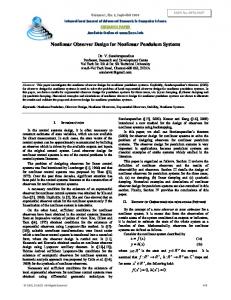
Then, the following system: xk , uk ) + g(yk , uk ) + X −1 Z (h(ˆ xk ) − yk ) , (38) x ˆk+1 = f (ˆ is an exponentially converging observer of system (35). Proof. The proof is similar to the proof of Theorem 3. V. S IMULATION Example 5.1: The following example has been served as a historical example to show hyper-chaos in electrical systems. 

−6  60 x˙ =   1 0 y = x1 ,

6 −2 −60 0 0 1 1.5 0

   0 2   −20   x +  −20  f (x1 , x2 ),   0 0  0 0 (39)

³ ´ where f (x1 , x2 ) = −1.6 |x2 − x1 − 1| − |x2 − x1 + 1| . This fourth order system contains a nonlinear elements and three-segment piecewise linear resistors. All the present elements are linear and passive, except an active resistor. We have chosen this particular system because it exhibits a nonlinearity with high Lipschitz constant. For all x ∈ IR4 , the Jacobian of the nonlinearity is     2 θ1 −θ1 0 0    ∂   −20  f (x1 , x2 ) =  θ2 −θ2 0 0  (x1 , x2 ),    0 0 0 0  0 ∂x 0 0 0 0 0 (40) where θ1 = 3.2 sign(x2 − x1 − 1) − 3.2 sign(x2 − x1 + 1), θ2 = −32 sign(x2 − x1 − 1) + 32 sign(x2 − x1 + 1) are bounded real-valued functions. Using the LMI package of

8209

FrC07.1 6

12 System Observer

System Observer

5

10

4

x4 and its estimate

x2 and its estimate

8 3

2

1

6

4

2 0

0

−1

−2

0

5

10

−2

15

0

5

10

Time in (sec)

Fig. 1.

15

Time in (sec)

The state x2 and its estimate

Fig. 3.

The state x4 and its estimate

2 System Observer

the output nonlinearity. By setting

0

x3 and its estimate

−2

f (x) =

"

2

e−x1 log(1 + x21 ) +

1 sin(x2 ) 2 x2

#

3 , x2 7 x2 − 1+x 2 − 4 1+x2 2 2 (43) ¸ · 1 0 , h(x) = x1 + sin(x1 ). g(y, u) = −0.1y 3 + u 2

−4

−6

−8

−10

0

5

10

The Jacobian of the aforementioned nonlinearity can be rewritten as follows

15

Time in (sec)

Fig. 2.

¸ · · ∂f (x) 1 0 0 + θ1,2 (x2 ) = F (θ) = θ1,1 (x1 ) 0 0 0 ∂x · ¸ 0 0 + θ2,2 (x2 ) 0 1

The state x3 and its estimate

MATLAB which gives us the following results: 



1.7154 0.1478 0.5658 −0.8385  0.1478 0.1658 0.0383 0.1070   P =  0.5658 0.0383 0.3936 −0.9189  , −0.8385 0.1070 −0.9189 13.7693   (41) −11.2540  −4.0597   Y =  2.4428  . −14.7078 In Figures 1, 2 and 3, we have represented the system states along with their estimates. The performance of the observer is clearly demonstrated as seen in the first instants of the simulations. Example 5.2: Now, we shall present an observation problem of a nonlinear system with a nonlinear output. Consider the following nonlinear system 2

x˙ 1 = e−x1 log(1 + x21 ) + x32

1 sin(x2 ) , 2 x2

x2 7 − − 0.1y 3 + u, 2 1 + x2 4 1 + x22 1 y = x1 + sin(x1 ). 2

x˙ 2 = −

(42)

1 0

¸

(44)

where 2

2

θ1,1 (x1 ) = −2x1 e−x1 log(1 + x21 ) + 2x1

e−x1 , 1 + x21

1 cos(x2 ) 1 sin(x2 ) − , 2 x2 2 x22 1 7x42 + 17x22 + 4 . θ2,2 (x2 ) = − 4 (1 + x22 )2

(45)

θ1,2 (x2 ) =

On the other hand, the output gradient can be rewritten in linear parameter varying form as ∂h(s) 1 = 1 + cos(s). ∂s 2

(46)

We have, −0.5 < |θ1,1 (x1 )| < 0.5, −0.5 < |θ1,2 (x2 )| < 0.5, −2 < |θ2,2 (x2 )| < −1 and 0.5 ≤ |ϑ1,1 (x1 )| ≤ 1.5. Using the LMI package of MATLAB, we get after solving the LMLs of Theorem 1 P =

where all the nonlinearities are globally Lipschitz including

8210

·

1.8928 0.6768 0.6768 4.7089

¸

, Y =

·

−6.87 1.3867

¸

.

(47)

FrC07.1 The nonlinear observer is readily constructed as 2 1 sin(ˆ x2 ) x ˆ˙ 1 = e−ˆx1 log(1 + x ˆ21 ) + 2 x ˆ2 ¡ ¢ 1 x1 ) − y , − 3.9371 x ˆ1 + sin(ˆ 2 ˆ32 x ˆ2 7 x ˙x − − 0.1y 3 + u ˆ2 = − 1+x ˆ22 41+x ˆ22 ¡ ¢ 1 + 0.8603 x ˆ1 + sin(ˆ x1 ) − y . 2 VI. C ONCLUSION

(48)

In this paper a useful and a simple design of nonlinear observers for systems having both nonlinear dynamics and nonlinear outputs is proposed. We showed that the design is free from any state transformation or linearization techniques generally employed for simplification of the observer analysis. Observer design with noise attenuation is also discussed in convex optimization setting. Examples showing the applicability and the efficiency of the design are given. R EFERENCES [1] S. Ibrir, “Less conservative linear matrix inequalities for observation of continuous-time and discrete-time nonlinear systems,” In proceedings of the first International Conference on Modelling, Simulation and Applied Optimization, Sharjah, United Arab Emirates, February 2005, paper 220. [2] R. E. Kalman, “A new approach to linear filtering and prediction problems,” Transactions of the ASME. Journal of basic engineering, vol. 82, no. D, pp. 35–45, 1960. [3] D. J. Luenberger, “An introduction to observers,” IEEE Transactions on Automatic Control, vol. AC-16, no. 6, pp. 596–602, December 1971. [4] F. E. Thau, “Observing the state of nonlinear dynamic systems,” International Journal of Control, vol. 17 , pp. 471–479, 1973. [5] J. P. Gauthier, H. Hammouri, and S. Othman, “A simple observer for nonlinear systems: Application to bioreactors,” IEEE Transactions on Automatic Control, vol. 37, no. 6, pp. 875–880, June 1992. [6] S. Raghavan and J. K. Hedrick, “Observer design for a class of nonlinear systems,” Int. J. Control, vol. 59, no. 2, pp. 515–528, 1994. [7] R. Rajamani, “Observers for Lipschitz nonlinear systems,” IEEE Transactions on Automatic Control, vol. 43, no. 3, pp. 397–400, 1998. [8] C. Aboky, G. Sallet, and L.-C. Vivalda, “Observers for Lipschitz nonlinear systems,” International Journal of control, vol. 75, no. 3, pp. 204–212, 2002. [9] S. Boyd, L. E. Ghaoui, E. Feron, and V. Balakrishnan, Linear matrix inequality in systems and control theory, ser. Studies in Applied Mathematics. SIAM, 1994. [10] M. Arcak and D. Neˇsi´c, “A framework for nonlinear sampled-data observer design via approximate discrete-time models and emulation,” Automatica, vol. 40, no. 11, pp. 1931–1938, 2004. [11] K. Reif and R. Unberhauen, “The extended kalman filter as an exponential observer for nonlinear systems,” IEEE Transactions on Signal processing, vol. 47, no. 8, pp. 2324–2328, August 1999. [12] K. Reif, S. G¨unther, E. Yaz, and R. Unbehauen, “Stochastic stability of the discrete-time extended Kalman filter,” IEEE Transactions on Automatic Control, vol. 44, no. 4, pp. 741–728, April 1999. [13] W. Lee and K. Nam, “Observer design for autonomous discrete-time nonlinear systems,” Systems & Control Letters, vol. 17, pp. 49–58, 1991. [14] G. Ciccarella, M. D. Mora, and A. Germani, “Observers for discretetime nonlinear systems,” Systems & Control Letters, vol. 20, pp. 373– 382, 1993. [15] P. E. Moraal and J. W. Grizzle, “Observer design for nonlinear systems with discrete-time measurements,” IEEE Transactions on Automatic Control, vol. 40, no. 3, pp. 395–404, March 1995. [16] S. Ibrir, W. F. Xie, and C.-Y. Su, “Observer-based control of discretetime Lipschitzian nonlinear systems: Application to one-link flexible joint robot,” International Journal of Control, vol. 78, no. 6, pp. 385– 395, April 2005.

[17] M. Arcak and P. Kokotovi´c, “Observer-based control of systems with slop-restricted nonlinearities,” IEEE Transactions on Automatic Control, vol. 46, no. 7, pp. 1146–1150, July 2001. [18] X. Fan and M. Arcak, “Observer design for systems with multivariable monotone nonlinearities,” Systems & Control Letters, vol. 50, pp. 319–330, 2003. [19] S. Ibrir, “Circle-criterion approach to discrete-time nonlinear observer design,” Automatica, vol. 43, no. 8, pp. 1432–1441, August 2007. [20] ——, “On-line exact differentiation and notion of asymptotic algebraic observers,” IEEE Transactions on Automatic Control, vol. 48, no. 11, pp. 2055–2060, 2003. [21] A. Alessandri, “Design of observers for Lipschitz nonlinear systems using LMI,” in NOLCOS, IFAC Symposium on Nonlinear Control Systems, Stuttgart, Germany, 2004. [22] E. E. Yaz and Y. I. Yaz, “LMI-based observer design for nonlinear systems with integral quadratic constraints,” IEEE Conference on Decision and Control, vol. 3, pp. 2954–2955, 2001. [23] A. Howell and J. K. Hedrick, “Design of observers for Lipschitz nonlinear systems using LMI,” in Proceedings of American Control Conference, vol. 3, Danvers, MA, USA, 2002, pp. 2088–2093. [24] H. Li and M. Fu, “A linear matrix inequality approach to robust H∞ filtering,” IEEE Transactions on Signal Processing, vol. 45, no. 9, pp. 2338–2350, 1997. [25] H. Nijmeijer and T. I. Fossen, New directions in non-linear observer design, ser. lecture notes in control and information sciences. Berlin: Springer, 1999, vol. 244. [26] A. J. Krener and M. Xiao, “Nonlinear observer design in the siegel domain,” SIAM Journal on Control and Optimization, vol. 41, no. 3, pp. 932–953, 2002. [27] A. J. Krener and W. Respondek, “Nonlinear observers with linearizable error dynamics,” SIAM J. Control and Optimization, vol. 23, no. 2, pp. 197–216, 1985. [28] X. H. Xia and W.-. B. Gao, “Nonlinear observer design by observer error linearization,” SIAM J. Control and Optimization, vol. 27, no. 1, pp. 199–216, January 1989. [29] J. M. Ortega and W. C. Rheinboldt, Iterative solution of nonlinear equations in several variables, SIAM ed., ser. Classics in Applied Mathematics, 2000, vol. 30. [30] P. Gahinet, A. Nemirovski, A. J. Laub, and M. Chilali, The LMI control toolbox, The Mathworks Inc., 1995. [31] P. Gahinet, P. Apkarian, and M. Chilali, “Affine parameter-dependent Lyapunov functions and real parametric uncertainty,” IEEE Transactions on Automatic Control, vol. 41, no. 3, pp. 436–442, 1996.

8211