LQN-Based Performance Evaluation Framework of UML-Based ...

LQN-Based Performance Evaluation Framework of UML-Based Models for Distributed Object Applications Ali I. El-Desouky Computers and Systems Department Faculty of Engineering Mansoura University Egypt

Hesham A. Ali Computers and Systems Department Faculty of Engineering Mansoura University Egypt [email protected]

Yousry M. Abdul-Azeem Computers and Systems Department Faculty of Engineering Mansoura University Egypt [email protected]

Model Driven Architecture (MDA) emphasizes the role of models as the primary artifacts of development by providing a set of guidelines for structuring specifications expressed as models and the transformations between such models [2]. The transformation maps the elements of a source model that conforms to a specific metamodel to elements of another model, the target model that conforms to the same or to a different metamodel. This paper proposes a framework that applies the model-driven principles in the context of performance engineering. The framework describes the transformation of a source software model, built by use of a software development tool, to a target performance model ready to be analyzed by a performance evaluation tool. Metamodeling techniques are used for defining the abstract syntax of software and performance models. The framework makes use of the set of MDA-related standards (MOF, QVT and XMI) to obtain a high degree of automation. The rest of this paper is organized as follows: MDA, MDA-related standards, and LQN are described briefly in section 2. Sections 3, 4 illustrate performance evaluation problem and the proposed framework. Sections 5, 6 presents the new implemented algorithms (SAT, ADLQNT). Section 7 discusses implementation issues in a case study and its performance results. Finally section 8 concludes our work and discusses future work.

Abstract Software Performance Engineering (SPE) has a great impact on software life cycle. A great effort had been introduced in this area. Automation degree of transformation and evaluation process, standardization degree, and performance parameters evaluated represent a big challenge for SPE. This paper presents an XSLTbased framework to overcome these challenges. This framework transforms Unified Modeling Language (UML) software models into Layered Queuing Networks (LQN) performance models. Such framework can be applied on distributed object applications (web services). What unify the proposed framework are: 1) the ability to use more than one type of UML diagrams in building Software model at first phase, 2) the standardization of algorithms applied because of applying XSLT / XQuery rules in all framework phases, 3) two new algorithms (SAT and ADLQNT) are used to achieve high automation degree of transformation and evaluation process, 4) the number of performance parameters evaluated at last phase, such as response time, throughput, and resource utilization before building the real program. Discussion and analysis of the proposed framework are based on illustrative example for validating its ability to achieve the proposed goal, and to evaluate its performance. Keywords: Software Performance Engineering SPE, UML, MDA, Meta Object Facility MOF, XML, Layered Queuing Networks LQN.

2. Model Driven Development (MDD) Model-driven development is simply the notion that it is possible to build an abstract model of a system that can be transformed into more refined models and eventually, into the system implementation. Model-driven development captures expert knowledge as mapping functions that, once executed, transform one model into another form [2]. The Object Management Group (OMG) addresses this notion with the Model Driven Architecture, which is at the core of model-driven development.

1. Introduction Software performance characteristics have the highest priority of software developers’ interest. Software Performance Engineering (SPE) assists in performance requirements validation [1]. To this purpose the performance engineering approach is applied throughout the development cycle by use of methods for building performance models from software development models. The obtained models can then be evaluated and their results checked against relevant performance requirements. INFOS2008, March 27-29, 2008 Cairo-Egypt © 2008 Faculty of Computers & Information-Cairo University SE-10

corresponding models at level 1 (e.g., UML models, which are instances of the UML metamodel). Finally, each model of level 1 describes concrete entities at level 0 (e.g., data described by a UML model).

2.1. Model Driven Architecture (MDA) MDA supports the development of software-intensive systems through the transformation of platformindependent models to platform specific models, executable components and applications. The motivation behind MDA is to transfer the focus of work from coding to modeling, by treating models as the primary artifacts of development. MDA provides a set of guidelines for structuring specifications expressed as models and the transformations between such models [3].

2.4. Query/View/Transformation (QVT) In response to the need for a standard approach to defining model transformations, the OMG issued the MOF QVT Final Adopted Specification [7]. The main requirement of QVT is to provide a standard for expressing transformations. QVT requires that model transformations be defined precisely in terms of the relationship between a source metamodel and a target metamodel. In some situations the source and target metamodels may be the same metamodel.

2.2. Unified Modeling Language (UML) UML is the OMG standard that helps in specifying, visualizing, and documenting models of software systems, including their structure and design, in a way that meets all of the needed requirements.  UML defines thirteen types of diagrams, divided into three categories [4]. 1. Structure Diagrams include the Class Diagram, Object Diagram, Component Diagram, Composite Structure Diagram, Package Diagram, and Deployment Diagram. 2. Behavior Diagrams include the Use Case Diagram, Activity Diagram, and State Machine Diagram. 3. Interaction Diagrams all derived from the more general Behavior Diagram; include the Sequence Diagram, Communication Diagram, Timing Diagram, and Interaction Overview Diagram. UML Profiles (that is, subsets of UML tailored for specific purposes) help in modeling Transactional, Realtime, and Fault-Tolerant systems. The recently adopted "UML Profile for Schedulability, Performance and Time SPT [5]" defines a general resource model, time modeling, general concurrency, schedulability and performance modeling. Chapter 7 of [5] defines the so-called Performance Profile dedicated to performance modeling, which provides mechanisms: • for capturing performance requirements, • for associating performance related QoS characteristics with the UML model, • for specifying execution parameters which can be used by modeling tools to compute predicted performance characteristics, • for presenting performance results computed by modeling tools or found by measurement.

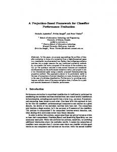
2.5. Layered Queuing Networks (LQN) Traditional Queuing Networks model is only a single layer of customer-server relationships. LQNs allow for an arbitrary number of client/server levels. LQNs can model intermediate software servers, and be used to detect software deadlocks and software as well as hardware performance bottlenecks. The layered aspect of LQNs makes them very suitable for evaluating the performance of distributed systems. LQNs model both software and hardware resources. The basic software resource is a task, which represents any software object having its own thread of execution. Tasks have entries that act as service access points. Each entry may consist of one or more activities processing concurrently or in sequence. The basic hardware resource is a device. Figure 1 shows the LQN visual notation [8, 9]. e1

Task

P1

Processor

e1

a

Entry

Activity

Synchronous request Asynchronous request Forwarding request

Figure1: LQN visual notation

3. Performance Evaluation Problem

2.3. Meta Object Facility (MOF)

Different methods of performance evaluation have been recently introduced. Their differences span from the type of input software models, to the type of output performance models, to the development cycle phase in which they can be applied, to the automation degree [10]. As an example, the source model could be either a model of UML type [11, 12, 13, 14] or not [15, 16] while the target model could be either a Layered Queuing Network [11, 15] or an Extended Queuing Network [13, 16] or a Stochastic Petri net [12, 17] or a stochastic process

MOF is the OMG standard that defines an abstract language and a framework for specifying, constructing, and managing technology neutral metamodels, (models used to describe other models) [6]. MOF introduces a four-level metadata architecture. At the metametamodel level 3, the MOF model is used to describe the metamodels at the lower level 2 (e.g. the UML metamodel, which is an instance of the MOF model). Level 2 metamodels are in turn used to describe the

SE-11

algebra [14]. Each one of those methods has one or more of the following drawbacks: • the method exhibits low automation degree, in other words much effort is required to implement the building method into an automatic tool; • the method has been implemented into a tool that is not easy to link to software development tools; • The method requires strong skills in performance theory to be effectively applied. The most recent approaches of performance evaluation are presented in table 1. For each one, types of UML diagrams used in software model, and performance parameters evaluated are shown. All approaches mentioned here uses UML software model as source model and LQN performance model as target model. Table 1: Summary of recent approaches Properties Approach

UML diagrams

4. Proposed Framework This paper introduces a facility to the modelers that use any type of UML diagrams to represent their models. These diagrams are then transformed, using the proposed Sequence to Activity Transformation (SAT) algorithm, into only two diagrams, a behavior one (Activity) and a Structure one (Deployment). Activity and Deployment to LQN Transformation (ADLQNT) algorithm is applied afterwards to get the performance model (represented in LQN). Highly automation degree is achieved here by these two newly implemented algorithms. A last step is to evaluate performance parameters from performance model; here we evaluate Utilization, Throughput, and Service time.

Performance Automation Parameters Degree

A Model-Driven Approach to Describe and Predict the Performance of Composite Services [11]

Class, Activity

Response time

Medium

Performance Analysis of Security Aspects in UML Models [18]

Sequence

Response time

Low

Early Performance Testing of Use Case, Latency, Distributed Software Deployment utilization Applications [19]

Low

Metadata-Driven Design of Activity, Throughput, Integrated Environments for Deployment Response Software Performance time Validation [20]

High

UML XMISchema

Validated by

Phase1

UML Tool

Phase2

Based on the comparison in table 1, it can be noticed that: 1. All approaches have used one or two UML diagrams at most to represent software model. 2. All approaches evaluate one or two performance parameters at most. 3. The automation degree in all these approaches differs from one approach to another spanning from low degree to high degree [10].

XML  Export 

XSLT/ XQuery Processor LQN Evaluation Tool

XMI

UML XMI-Docs XMI

XSLT/  XQuer l

UML Instance UML Model Meta-Model of

Transformation Algorithms

SA

ADLQN

LQN

XML  XMI-Docs XMI Import 

Instance of

LQN LQN Instance Meta-Model Model of

Validated by

Phase3

Model Transformation

Meta-Model Transformation

Model files flow

Figure 2: Proposed framework

SE-12

QV T XMI

LQN XMISchema

Instance  of

MO

Figure 2 shows the proposed framework for performance evaluation. The framework is divided into three phases. Each phase has its function and its own algorithms. The proposed framework has the following characteristics: 1) The ability to use more than one type of UML diagrams in building Software model at first phase. 2) The standardization of algorithms applied because of applying XSLT / XQuery rules in all framework phases [21]. 3) Two new algorithms (SAT and ADLQNT) are used to achieve high automation degree of transformation and evaluation process. 4) The number of performance parameters evaluated at last phase. To support the entire scope of transformation process, this framework is designed as a suite of algorithms distributed into its three main phases.

provides more direct ways of modeling; concurrent forks and joins; hierarchal scenarios. Other Diagrams

UML Model (Input) Interaction Coll. or Seq.?

Export from tool as Sequence

Step 1

Activity

Collaboration

Deployment

Out of our scope

Sequence

SAT 

Activity

Step 2

4.1. Phase One (Building and Validating the UML Model)

Annotate with S.W. PerformanceRelated Values

Annotate with H.W. PerformanceRelated Values

XMI

XMI

Model in XML file Applying XSLT rules

A UML CASE Tool [22] is used to build the UML Model, flexibility of building the model using only two UML Diagrams or more is provided. UML Model is then exported into XMI Documents [23]. In order to standardize these XMI-Documents, XSLT rules are applied using a standard XSLT/XQuery Processor [21]. XMI Documents are then validated using UML XMI Schema that is exported from the UML Meta-Model of the system. A UML Meta-Model is used to define how UML model is transformed and as a reference point against which the model transformation is checked.

ADLQNT  Step 3

LQN Model (Output)

Figure 3: Transformation Steps Step Two (Annotate Diagrams with PerformanceRelated Values). Performance measures for a system include resource utilizations, waiting times, execution demands (for CPU cycles or seconds) and response time, (the actual time to execute a scenario or scenario step). Each measure may be defined in different versions, several of which may be specified in the same model, such as; (required value, coming from the system requirements or from a performance budget based on them (e.g., a required response time for a scenario), assumed value, based on experience (e.g., for an execution demand or an external delay), estimated value, calculated by a performance tool and reported back into the UML model, measured value) [5]. Activity and Deployment Diagrams are annotated with performance parameters. Each parameter is specified as one of these types for example ( {PAdemand = (‘assm’, ’mean’, 1.5,’ ms)}). This means the execution time of this step is assumed mean of 1.5 milliseconds.

4.2. Phase Two (Transformation) As shown in Figure 3, the second phase of the framework consists of three main steps as follow: Step One (From Behavior Diagram to Activity Diagram). Sequence and Collaboration Diagrams are transformed into Activity Diagram as an example in this approach. The main goal of this step is to minimize UML Diagrams types used in performance evaluation by applying SAT algorithm. For the sake of performance annotation, we need here two types of diagrams a Behavior one (Use Case Diagram, Activity Diagram, State Machine Diagram, Sequence Diagram, Communication Diagram, Timing Diagram, or Collaboration Diagram), and a Structure one (Class Diagram, Object Diagram, Component Diagram, Composite Structure Diagram, Package Diagram, or Deployment Diagram). Activity and Interaction (Sequence or Collaboration) Diagrams are usually used to represent scenarios also Statecharts are another kind of diagrams for behavior description but it doesn’t illustrate the cooperation between several objects, so it isn’t appropriate for describing scenarios. Activity diagram

Step Three (From Activity & Deployment to LQN). The goal of this step is to transform the Activity Diagram, produced from the previous phase or entered in the first one, with the Deployment Diagram into LQN performance model, in order to measure or evaluate performance parameters. This transformation is done by applying ADLQNT algorithm.

SE-13

4.3. Phase Three (Building the LQN Model and measuring the Performance)

a

b idle

invoke(x( ))

An XMI-Document containing the resulted LQN model is received at the end of the transformation process. The model is then checked against the LQN metamodel (LQN XMI schema file). LQN model can be solved either by the analytical solver LQNS or simulation solver LQSim [24]. LQNS solves models mathematically, and is faster than LQSim. LQSim takes longer time to solve model, but gives more accurate results for complex models. Performance parameters such as resource utilization, throughput, and response time are evaluated here; it also can be examined against the required performance matrices that software developers need to achieve them.

a:A

b:B x( ) x( ) rep

return(rep)

receive(rep)

(A)- Synchronous message Send and reply transformation a a:A

b:B x( )

5. Sequence to Activity Transformation algorithm (SAT) SAT is an XMI-Based transformation algorithm from Sequence diagrams to Activity diagrams. It takes an XMIDocument containing Sequence diagram as an input. After applying the algorithm, an XMI-Document containing the resulted activity diagram is resulted as an output. The CASE Tool used in the transformation process exports both Sequence and Collaboration diagrams as one model in XML-Document. The concentration here will be on Sequence diagrams and Collaboration diagrams will be exported as Sequence diagram using this tool. The concept behind the transformation is to follow the flow of messages in a sequence diagram, considering the execution threads of all active objects involved in the collaboration. The main messages cases are: 1. A synchronous message between objects running in different threads of control. 2. An asynchronous message sent to another thread of control. In the first case a message is transformed as a join operation on the receiving side, and its reply marks the corresponding fork Figure 4-A. The sender thread will be blocked until the reply is received back. In the second case the message is transformed into a join operation on the receiver side, and a fork operation on the sender side Figure 4-B. The resulted activity diagram contains separate swimlans for each active object to show actions performed by this object and its associated passive objects.

b idle

invoke(x( ))

x( )

(B)- Asynchronous message transformation

Figure 4: Message transformation from Sequence to Activity Diagram SAT algorithm is executed here to create a new model to represent the equivalent activity diagram. A segment of code demonstrates the steps of SAT algorithm is shown below: public void doSAT() { loadSequenceGraph(XMLfile); createPartitions(); initializePartitions(); sortAndTransformMsgs(); finalizePartitions(); setActivityGraph(); } The algorithm execution sequence will be carried out as follows: 1- Load XML-file that contains the sequence diagram. 2- Create partition for each active object using object data. 3- Initialize each partition with an initial state, init pseudostate for first partition, and idle actionstate for other partitions.

SE-14

4- Sort messages using their stereotypes and specify concurrent messages. 5- Transform messages, using their types, into actions (CallAction or SendAction). For both of them, actionstates are created and given names. CallAction is synchronous, the caller is blocked and yields control to the called procedure until it returns. It is assumed in UML notation that every call has a paired return. SendAction is asynchronous, resulting in an explicit fork. 6- Update partitions’ contents with states and insert transitions between these states. 7- Use the current data to write the activity diagram into XMI-Document.

loadDeployment(DepFile); for each(node in deployment) if(device) createTask(node); elseif(processor) createProcessor(node); elseif(process) createTaskforProcessor(node); }

7. Case Study Discussion and Analysis 6. Activity and Deployment Diagrams to LQN Transformation algorithm (ADLQNT)

A case study is used to test our framework. This case study is a simulation for a book store system. In this scenario, user accesses a web page and gets book information. System hardware contains three servers,as shown in deployment diagram Figure 5, two of them are web servers (WebServer, BookStore Server), and the other one is Database server. On web server a web service is hold, invokes getBookInfo() method on Bookstore Server and returns Book information. On Bookstore Server a web service is used to invoke getPriceInfo() method and to get price info from Database Server. On Database Server book pricing data is stored

ADLQNT algorithm takes performance-annotated activity and deployment diagrams as an input. It uses these diagrams to build LQN model. First let’s introduce the main components of each diagram and the equivalent LQN component that it will be transformed into. Deployment Diagram. The main component of any deployment diagram is Node which can have Device or Processor stereotype. A Node with stereotype processor is transformed into LQN processor, while a Node with stereotype Device is transformed into LQN Task. Activity Diagram. The main components of any activity diagram are; Partition, ActionState, Transition, PseudoState. For each we will introduce a transformation to LQN components. Partition is transformed into LQN component Task. ActionState whose incoming Transition instance connects it with an ActionState or PseudoState within different Partition is transformed into LQN Entry. ActionState whose incoming Transition instance connects it with an ActionState or PseudoState within the same Partition is transformed into LQN Activity. ActionState whose incoming Transition corresponds to a call return is transformed into LQN Activity. Transition connecting actions in different partitions are transformed into LQN Call, specifically synchcall or asynch-call corresponding to the Transition of message type. Other Transitions are neglected. PseudoStates is not transformed to any LQN components, it is rather treated as a control node that aids in transformation process. A segment of code demonstrates the ADLQN algorithm is shown below:

 

 

  webServer CPU

User CPU 

Internet 

  Browser

 

 

  webServer

 

DBServer CPU 

DBServer  Disk

 

DBserver  

 

Book‐Store  Server Disk

LAN 

  BookStoreServer CPU   bookstore  

Server

Figure 5: Deployment Diagrams System sequence is shown in sequence diagram of figure 6. User requests book information, using his browser, from webserver. getPriceInfo() method is invoked to get book description from bookstore server disk. Book store server invokes getPriceInfo() to get book-pricing data from DBserver disk. BookStore server returns bookInfo() to webserver on which an

Public void doADLQNT() { loadActivityGraph(ActvFile);

SE-15

HTML page containing book information is created. This HTML page is returned to the user browser to be displayed. Applying SAT algorithm, the resulted Activity diagram will be as shown in Figure 7. Using Deployment diagram and the resulted Activity diagram as inputs for ADLQNT algorithm, the resulted LQN will be as shown in Figure 8.

Web Server

Browser

1: request‐ Book( ) 

Book‐Store Server 

2: getBookInfo( ) 

3: getPriceInfo( )

4: priceInfo( ) 5: bookInfo( )  6: generate‐  HTML( )  7: display‐ HTML( )

Figure 6: Sequence Diagram Browser 

DB Server

WebServer

BookStoreServer

DBServer 

init

Idle

Idle

invoke(requestBook( ))

Idle requestBook( ) invoke(getBookInfo( )) getBookInfo( ) invoke(getPriceInfo( )) getPriceInfo( ) return(priceInfo( ))

priceInfo( ) return(bookInfo( ))

bookInfo( ) generateHTML( ) return(HTML)

displayHTML( )

Figure 7: Activity Diagram

SE-16

Invoke(requestBook() Internet

Internet

displayHTML( )

User CPU

requestBook( )

Browser

Internet

invoke(getBookInfo( )) getBookInfo ( )

BookStore Disk

receive(bookInfo( )) invoke(getPriceInfo( ))

BookStore Disk Book Store Disk

LAN Entry

receive(priceInfo( ))

LAN getPriceInfo( )

return(displayHTML( ))

return(bookInfo( ))

LAN

BookStore

return(priceInfo( ))

DBServer DBDisk Entry DBServer CPU

generateHTML( )

BookStore Server CPU

WebServer WebServer CPU

DBDisk DBdisk

Figure 8: Resulted LQN Diagram •

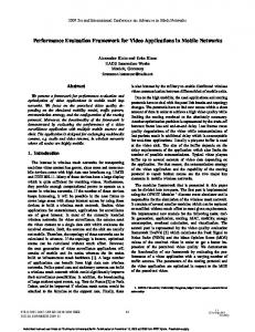
Response time: the time a system or a part of it takes to respond for a request. Service time can be defined as the sum of response time and request time, and assuming that request time is fixed we can use service time in our measurements. When applying framework steps on the system, measured values of throughput, utilization, and service time against number of users accessing the system are resulted. Throughput: in Figure 9 throughput of the system is represented as sum of total throughputs of each component in the system, measured by number of jobs done in milliseconds.

7.1. Performance analysis and results Here we have to notice the main performance parameters that are useful in building software programs: • Throughput: it is the rate at which a computer or network sends or receives data. In computer technology, throughput is the amount of work that a computer can do in a given time period. Throughput theoretically tells how much useful work the system is producing. • Utilization: is the ratio of time a system is busy divided by the time it is available. For example, if a system was available for 160 hours and busy for 40 hours, then utilization was (40/160 =) 0.25.

SE-17

Figure 9: Throughput vs. Number of clients Figure11: Service time vs. Number of clients

As seen from the figure, increasing the number of users increases throughput till it reaches a specific value (5 users). Utilization: in Figure 10 utilization is represented for each server or service in the system as sum of components utilization of each one. Increasing number of users increases utilization till it reaches a specific value (25 users).

8. Conclusion and future work In this paper the problem of automatic performance evaluation of software systems is addressed. A new XSLT-based framework is introduced in three phases for transforming Software model, represented in UML diagrams, into Performance model, represented in LQN, in order to evaluate performance parameters. Two new algorithms are also represented to achieve highly degree of automation in the system. SAT algorithm which transforms Sequence diagram into Activity diagrams. ADLQNT algorithm which transforms Activity and Deployment to LQN model. A case study with a web service scenario is used to implement issues of the proposed framework and results are observed and recorded for comparison. As future work, we plan to complete the implementation of third phase of framework with proposing a new algorithm in reading the performance parameters from LQN and take it as a feedback, as it's the most important and challenging task to enhance the current model performance before writing the software code.

References Figure 10: utilization vs. Number of clients

[1] C. U. Smith, Performance Engineering of Software Systems, Addison-Wesley, MA, 1990. [2] S.J. Mellor, A.N. Clark, T. Futagami. Model-driven development. IEEE Software Special Issue, vol 20, n. 5, September 2003. [3] Object Management Group, MDA Guide. version 1.0.1, June 2003. [4] Object Management Group: Unified Modeling Language (UML): Superstructure. Version 2.0, 2005. [5] Object Management Group: UML Profile for Scheduling, Performance and Time. Version 1.1, 2005. [6] Object Management Group, Meta Object Facility (MOF) Core Specification. version 2, April 2006.

Service time: it is also represented as the sum of all system components service time. It has a linear behavior as shown in figure 11. That is true since every server and service has constant service time except the user processor which is increasing at each measure. This leads to increase service time and its linearity behavior.

SE-18

[7] Object Management Group. Meta Object Facility (MOF) 2.0 Query/View/Transformation Specification. 2005. [8] G. Bolch, S. Greiner, H. de Meer, and K. S. Trivedi: Queueing Networks and Markov Chains: Modeling and Performance Evaluation with Computer Science Applications, 2nd Edition. Wiley–Interscience, 2006. [9] J.A. Rolia, K.C. Sevcik. The Method of Layers. IEEE Trans. On Software Engineering, Vol. 21, Nb. 8, pp 689700, August 1995. [10] S. Balsamo, A. Di Marco, P. Inverardi, M. Simeoni, Model-Based Performance Prediction in Software Development: A Survey. IEEE Transactions on Software Engineering, vol. 30, n. 5, pp. 295-310, 2004. [11] A. D’Ambrogio, P. Bocciarelli. A Model-driven Approach to Describe and Predict the Performance of Composite Services. Proceedings of the sixth Workshop on Software Performance (WOSP’07), P 78-89, February 2007. [12] J. M. Fernandes, S. Tjell, J. B. Jørgensen, O. Ribeiro. Designing Tool Support for Translating Use Cases and UML 2.0 Sequence Diagrams into a Coloured Petri Net. Sixth International Workshop on Scenarios and State Machines (SCESM'07), 2007. [13] V. Cortellessa, R. Mirandola, PRIMA-UML: a performance validation incremental methodology on early UML diagrams. Science of Computer Programming, vol. 44, pp. 101–129, 2002. [14] R. Pooley, Using UML to Derive Stochastic Process Algebra Models. Proceedings of the XV UK Performance Engineering Workshop, 1999. [15] V. Cortellessa, A. D’Ambrogio, G. Iazeolla, Automatic Derivation of Software Performance Models from CASE documents. Performance Evaluation, 45(2-3):81–106, July 2001. [16] A. D’Ambrogio, G. Iazeolla, Steps towards the Automatic Production of Performance Models of Web Applications. Computer Networks Journal, vol. 41, pp. 29–39, January 2003. [17] J.P. Lpez-Grao, J. Merseguer, J. Campos, From UML Activity Diagrams to Stochastic Petri Nets: Application to Software Performance Engineering. Proceedings of the Fourth Workshop on Software and Performance (WOSP’04), Redwood City, CA, USA, January 2004. [18] D.C. Petriu, C.M. Woodside, D.B. Petriu, J. Xu, T. Israr, Performance Analysis of Security Aspects in UML Models. Proceedings of the sixth Workshop on Software Performance (WOSP’07), P 91-102, February 2007 [19] G. Denaro, A. Polini, W. Emmerich, Early Performance Testing of Distributed Software Applications, Proceedings of the fourth Workshop on Software Performance, (2004). [20] G. P. Gu, D. C. Petriu, From UML to LQN by XML algebra-based model transformations, Proceedings of the fifth Workshop on Software Performance, (2005). [21] WWW Consortium, eXtensible Stylesheet Language: Transformations (XSLT), W3C Recommendation, http://www.w3.org/TR/xslt. [22] IBM, Rational Rose Enterprise Edition. http://www306.ibm.com/software/rational/. [23] Object Management Group, XML Metadata Interchange (XMI) Specification. version 2.0, May 2003. [24] −, LQN Online Documentations, http://www.sce.carleton.ca/rads/lqn/lqn-documentation.

SE-19